


1. Introduction
Following quantum mechanics’ genesis, the study of precisely solvable problems plays a critical role in comprehending the underlying quantum-mechanical systems [1–3]. Analytical solutions of the Schrödinger, Klein–Gordon (KG), and Dirac equations are of particular importance in quantum mechanics because the wave function contains all the information necessary for a complete description of a particle’s behaviour in a force field [3–8].
In any n radial and l orbital quantum states, a limited number of physical potentials can be solved exactly for the Schrödinger, KG, and Dirac equations [2, 3]. Generally, many quantum systems can only be solved numerically or through approximation techniques [7–9]. Therefore, several methods including the supersymmetry method [10], the factorisation method [3], the Laplace transform approach [11], the path integral method [12], the Nikiforov–Uvarov (NU) method [13], asymptotic iteration method [14, 15] and the quantisation rule method [16–18] have been developed so far and they have been applied for the solution of the quantum wave equation. The NU method yields more practicality to solve second-order differential equations by transforming them into hypergeometric-type equations. Furthermore, the various exponential and hyperbolic potentials are analytically solved by using different approximation schemes with the NU method.
In principle, the exponential potential models always draw considerable attention and are widely used in various physical systems, including quantum cosmology, nuclear physics, molecular physics, elementary particle physics, and condensed matter physics [19–29]. Up to now, many exponential-type potentials, including the Morse [30, 31], Hulthén [32–38], Woods–Saxon [27, 39–43], Rosen–Morse [44–48], Eckart-type [49–51], Manning–Rosen [52–54], Deng–Fan [55, 56], Pöschl–Teller like [57], Mathieu [58], sine-type hyperbolic [59] and Schiöberg [60–63] potentials have been investigated, and some analytical bound state solutions were obtained using an approximation for these models in l ≠ 0 state. Some known exponential potentials can also be transformed into a hyperbolic potential model, which can help understand quantum systems’ natural dynamics [64–76]. For instance, the thermodynamic properties of some molecules have been successfully predicted using the improved Rosen–Morse potential and the Fu-Wang-Jia potential to describe the internal vibrations of molecules [77–82].
Motivated by the simplicity and applicability of the generalisations of the hyperbolic potentials, the generalised tanh-shaped hyperbolic potential (GTHP) [83] was recently proposed as follows:
$\begin{eqnarray}V(r)={V}_{1}+{V}_{2}\tanh (\alpha r)+{V}_{3}{\tanh }^{2}(\alpha r),\end{eqnarray}$
where V1, V2, V3 are the depths of potential well and α is the adjustable parameter representing the properties of the interaction potential. For clarity about potential, see also the S2 section4(4See supplementary material, which includes [29, 56, and 63], for additional details of potential information and theoretical derivations.). GTHP is the general case of the significant physical potential such as the standard and generalised Woods–Saxon [39, 42], Rosen–Morse [44], Manning–Rosen type, generalised and standard Morse [30], Schiöberg [60], four-parametric exponential-type [67–69], Williams–Poulios potential [84, 85], and the sum of the linear and harmonic oscillator potentials, see S2 section in4. As it seems, GTHP’s characteristics can be used to explain the interactions of molecular, atomic, and nuclear particles.In this study, we extend our study of GTHP by considering it in the KG equation. We apply the NU method to analytically solve KG and obtain the bound state for this potential, and we compare the results with the previously reported ones in particular cases. Then, the potential is modelled for several diatomic molecules, and the obtained results are in good agreement with experimental ones. This study allows us to correctly explain a broad variety of quantum systems’ characteristics and behaviour, including retardation effects, without needing a great deal of complex derivation or massive computing resources. The remainder of this study covers the following sections: the bound-state solution of the radial KG equation is presented in section 2 . In section 3 , we explore the results for energy levels and the corresponding normalised eigenfunctions in some special cases and diatomic molecules. Finally, some concluding remarks are stated in section 4 .
2. Bound state solutions
The time-independent KG equation with scalar and vector potentials S(r) and V(r) a spin-zero particles takes the general form: [2]2 ), the modified radial KG equation is obtained as follows:4 ) becomes in the following form:1 ), that is
$\begin{eqnarray}\begin{array}{l}{{\rm{\nabla }}}^{2}\psi (r,\theta ,\varphi )+\displaystyle \frac{1}{{\hslash }^{2}{c}^{2}}\{{\left(E-V(r)\right)}^{2}\\ \,-{\left({{Mc}}^{2}+S(r)\right)}^{2}\}\psi (r,\theta ,\varphi )=0,\end{array}\end{eqnarray}$
where E is the relativistic energy system an M denotes the rest mass of the particle. To denote the radial and angular components of the wave function ψnlm(r, θ, φ), the concept of variable separation is defined as: $\begin{eqnarray}{\psi }_{{nlm}}(r,\theta ,\varphi )=\displaystyle \frac{{\chi }_{{nl}}(r)}{r}{{\rm{Y}}}_{{lm}}(\theta ,\varphi ),\end{eqnarray}$
and substituting it into equation ( $\begin{eqnarray}\left[\frac{{{\rm{d}}}^{2}}{{\rm{d}}{r}^{2}}+\frac{(E-{{Mc}}^{2}-V(r)-S(r))(E+{{Mc}}^{2}-V(r)+S(r))}{{\hslash }^{2}{c}^{2}}-\frac{l(l+1)}{{r}^{2}}\right]\chi (r)=0.\end{eqnarray}$
After choosing of equal scalar and vector potentials, that is, S(r) = V(r), equation ( $\begin{eqnarray}\begin{array}{l}\frac{{{\rm{d}}}^{2}\chi (r)}{{\rm{d}}{r}^{2}}+\frac{1}{{\hslash }^{2}{c}^{2}}\\ \times \,\left[{E}^{2}-{M}^{2}{c}^{4}-2(E+{{Mc}}^{2})V(r)-\frac{{\hslash }^{2}{c}^{2}l(l+1)}{{r}^{2}}\right]\chi (r)=0.\end{array}\end{eqnarray}$
Considering the expression of 2V(r) equal as equation ( $\begin{eqnarray}2V(r)={V}_{\mathrm{GTHP}}(r)={V}_{1}+{V}_{2}\tanh (\alpha r)+{V}_{3}{\tanh }^{2}(\alpha r).\end{eqnarray}$
It should be noted that this choice the potential enables us to reduce the resulting relativistic states to their non-relativistic limit under appropriate transformations. Therefore, we obtain it as:8 ) into equation (7 ), and further using a new variable $\tanh (\alpha r)=s$, s ∈ [0, 1], we obtain it as:10 ) should be rewritten as the hypergeometric type equation form as:
$\begin{eqnarray}\begin{array}{l}\frac{{{\rm{d}}}^{2}\chi (r)}{{\rm{d}}{r}^{2}}+\frac{1}{{\hslash }^{2}{c}^{2}}\{{E}^{2}-{M}^{2}{c}^{4}-(E+{{Mc}}^{2})\\ \ \ \times \,[{V}_{1}+{V}_{2}\tanh (\alpha r)+{V}_{3}{\tanh }^{2}(\alpha r)]\\ \,-\frac{{\hslash }^{2}{c}^{2}l(l+1)}{{r}^{2}}\}\chi (r)=0.\end{array}\end{eqnarray}$
This equation cannot be solved analytically for l ≠ 0 due to the centrifugal term. Therefore, the Pekeris approximation [40–42, 83, 86] which is the most widely used and convenient for our purposes can be taken to solve this equation. According to the Pekeris approximation scheme to deal with the centrifugal term is used [83] $\begin{eqnarray}\displaystyle \frac{1}{{r}^{2}}\approx \displaystyle \frac{1}{{r}_{e}^{2}}[{A}_{0}+{A}_{1}\tanh (\alpha r)+{A}_{2}{\tanh }^{2}(\alpha r),\end{eqnarray}$
where the parameters A0, A1 and A2 were found as: [83] $\begin{eqnarray}\left\{\begin{array}{l}{A}_{0}=1+\tfrac{{\cosh }^{4}(\alpha {r}_{e})}{{\alpha }^{2}{r}_{e}^{2}}[3{\tanh }^{2}(\alpha {r}_{e})+2\alpha {r}_{e}\tanh (\alpha {r}_{e})(1-2{\tanh }^{2}(\alpha {r}_{e}))]\\ {A}_{1}=-\tfrac{2{\cosh }^{4}(\alpha {r}_{e})}{{\alpha }^{2}{r}_{e}^{2}}[3\tanh (\alpha {r}_{e})+\alpha {r}_{e}(1-3{\tanh }^{2}(\alpha {r}_{e}))]\,\,\,\,\,\,.\\ {A}_{2}=\tfrac{{\cosh }^{4}(\alpha {r}_{e})}{{\alpha }^{2}{r}_{e}^{2}}(3-2\alpha {r}_{e}\tanh (\alpha {r}_{e})).\end{array}\right.\end{eqnarray}$
After inserting the equation ( $\begin{eqnarray}\chi ^{\prime\prime} (s)-\displaystyle \frac{2s}{1-{s}^{2}}\chi ^{\prime} (s)-\displaystyle \frac{\varepsilon +\beta s+\gamma {s}^{2}}{{\left(1-{s}^{2}\right)}^{2}}\chi (s)=0,\end{eqnarray}$
where $\begin{eqnarray}\left\{\begin{array}{l}\tfrac{{E}^{2}-{M}^{2}{c}^{4}-(E+{{Mc}}^{2}){V}_{1}}{{\alpha }^{2}{\hslash }^{2}{c}^{2}}-\tfrac{l(l+1){A}_{0}}{{\alpha }^{2}{r}_{e}^{2}}=-\varepsilon \\ \tfrac{(E+{{Mc}}^{2}){V}_{2}}{{\alpha }^{2}{\hslash }^{2}{c}^{2}}+\tfrac{l(l+1){A}_{1}}{{\alpha }^{2}{r}_{e}^{2}}=\beta \\ \tfrac{(E+{{Mc}}^{2}){V}_{3}}{{\alpha }^{2}{\hslash }^{2}{c}^{2}}+\tfrac{l(l+1){A}_{2}}{{\alpha }^{2}{r}_{e}^{2}}=\gamma \end{array}\right.\end{eqnarray}$
with the boundary conditions χ(0) = 0 and χ(1) = 0. Now for implementing the NU method, equation ( $\begin{eqnarray}\chi ^{\prime\prime} (s)+\displaystyle \frac{\tilde{\tau }(s)}{\sigma (s)}\chi ^{\prime} (s)+\displaystyle \frac{\tilde{\sigma }(s)}{{\sigma }^{2}(s)}\chi (s)=0.\end{eqnarray}$
After comparing equation (10 ) and equation (12 ), we obtain:13 ) and taking $\sigma ^{\prime} (s)=-2s$. Hence, the function π(s) is defined as:14 ) under the square root is equal to zero. Hence, we obtain it as:15 ) are substituted into equation (14 ), the eight possible forms of π(s) are written in the following forms:19 ) with equation (20 ), we obtain the following relation:
$\begin{eqnarray}\tilde{\tau }(s)=-2s;\,\sigma (s)=1-{s}^{2};\,\tilde{\sigma }(s)=-\varepsilon -\beta s-\gamma {s}^{2}.\end{eqnarray}$
The new function π(s) as given in [13] can be obtained by substituting equation ( $\begin{eqnarray}\pi (s)=\pm \sqrt{(\gamma -k){s}^{2}+\beta s+\varepsilon +k}.\end{eqnarray}$
The value of the constant parameter k can be calculated by performing the condition that the discriminant of the expression equation ( $\begin{eqnarray}\left\{\begin{array}{l}{k}_{1}={D}^{2}-\varepsilon ,\\ {k}_{2}={P}^{2}-\varepsilon ,\end{array}\right.\end{eqnarray}$
where $\begin{eqnarray}\left\{\begin{array}{l}D=\sqrt{\tfrac{(\varepsilon +\gamma )+\sqrt{{\left(\varepsilon +\gamma \right)}^{2}-{\beta }^{2}}}{2}},\\ P=\sqrt{\tfrac{(\varepsilon +\gamma )-\sqrt{{\left(\varepsilon +\gamma \right)}^{2}-{\beta }^{2}}}{2}}\end{array}\right.\end{eqnarray}$
with D > P, 2DP = ∣β∣, D2 + P2 = ϵ + γ. When the individual values of k are given in equation ( $\begin{eqnarray}\pi (s)=\pm \left\{\begin{array}{c}{Ps}\pm D,\,{for}\,\,k\,=\,{D}^{2}-\varepsilon \\ {Ds}\pm P,\,{for}\,\,k\,=\,{P}^{2}-\varepsilon \,\end{array}\right..\end{eqnarray}$
Even π(s) have eight different values, but according to NU method, we select only one of them such that the function $\tau (s)=\tilde{\tau }(s)+2\pi (s)$ has the negative derivative and a root on the interval (0, 1), that is, $\tau ^{\prime} (s)\lt 0$ and τ(s) = 0, s ∈ (0, 1). Noticing that the other forms have no physical meaning, we will take: $\begin{eqnarray}\left\{\begin{array}{l}\pi (s)=P-{Ds}\\ \tau (s)=2P-2(D+1)s\\ k\,=\,{P}^{2}-\varepsilon \end{array}\right..\end{eqnarray}$
After using the following relations: $\lambda =k+\pi ^{\prime} (s)$ and ${\lambda }_{n}=-n\tau ^{\prime} (s)-\tfrac{n(n-1)}{2}\sigma $, (n = 0, 1, 2,….) [13], we obtain λ as: $\begin{eqnarray}\lambda =k+\pi ^{\prime} (s)={P}^{2}-\varepsilon -D\end{eqnarray}$
and $\begin{eqnarray}\lambda ={\lambda }_{n}=2{Dn}+n(n+1),\end{eqnarray}$
where n is the radial quantum number (n = 0, 1, 2,….). After comparing equation ( $\begin{eqnarray}D=n^{\prime} \gt 0,\end{eqnarray}$
where $\begin{eqnarray}n^{\prime} =\sqrt{\displaystyle \frac{1}{4}+\gamma }-n-\displaystyle \frac{1}{2}.\end{eqnarray}$
By inserting the expression D into equation (21 ) we obtain11 ) and (22 ) into equation (23 ) for energy level equation, we obtain it as:
$\begin{eqnarray}\varepsilon +\beta +\gamma ={\left(n^{\prime} +\displaystyle \frac{\beta }{2n^{\prime} }\right)}^{2}.\end{eqnarray}$
After inserting the equations ( $\begin{eqnarray}\begin{array}{l}{M}^{2}{c}^{4}-{E}^{2}+(E+{{Mc}}^{2})({V}_{1}+{V}_{2}+{V}_{3})\\ \ \ +\,\displaystyle \frac{{\hslash }^{2}{c}^{2}l(l+1)}{{r}_{e}^{2}}({A}_{0}+{A}_{1}+{A}_{2})={\alpha }^{2}{\hslash }^{2}{c}^{2}\\ \ \ \times \,\left[\Space{0ex}{5.25ex}{0ex}\sqrt{\displaystyle \frac{(E+{{Mc}}^{2}){V}_{3}}{{\alpha }^{2}{\hslash }^{2}{c}^{2}}+\displaystyle \frac{l(l+1)}{{\alpha }^{2}{r}_{e}^{2}}{A}_{2}+\displaystyle \frac{1}{4}}\right.\\ \ \ {\left.-\,n-\displaystyle \frac{1}{2}+\displaystyle \frac{\tfrac{(E+{{Mc}}^{2}){V}_{2}}{2{\alpha }^{2}{\hslash }^{2}{c}^{2}}+\tfrac{l(l+1)}{2{\alpha }^{2}{r}_{e}^{2}}{A}_{1}}{\sqrt{\tfrac{(E+{{Mc}}^{2}){V}_{3}}{{\alpha }^{2}{\hslash }^{2}{c}^{2}}+\tfrac{l(l+1)}{{\alpha }^{2}{r}_{e}^{2}}{A}_{2}+\tfrac{1}{4}}-n-\tfrac{1}{2}}\right]}^{2}.\end{array}\end{eqnarray}$
with n = 0, 1, 2,... $\unicode{x0230A}\sqrt{\tfrac{(E+{{Mc}}^{2}){V}_{3}}{{\alpha }^{2}{\hslash }^{2}{c}^{2}}+\tfrac{l(l+1)}{{\alpha }^{2}{r}_{e}^{2}}{A}_{2}+\tfrac{1}{4}}-\tfrac{1}{2}-\sqrt{-\tfrac{(E+{{Mc}}^{2}){V}_{2}}{2{\alpha }^{2}{\hslash }^{2}{c}^{2}}-\tfrac{l(l+1)}{2{\alpha }^{2}{r}_{e}^{2}}{A}_{1}}\unicode{x0230B}$.By applying the NU method, we can obtain the radial eigenfunctions. After substituting π(s) and Σ(s) into $\tfrac{{\rm{\Phi }}^{\prime} (s)}{{\rm{\Phi }}(s)}=\tfrac{\pi (s)}{\sigma (s)}$ and $\tfrac{\rho ^{\prime} (s)}{\rho (s)}+\tfrac{\sigma ^{\prime} (s)}{\sigma (s)}=\tfrac{\tau (s)}{\sigma (s)}$ solving the order differential equation, one can find the finite function Φ(s) and ρ(s) in the interval (0, 1) it is easily obtained:
$\begin{eqnarray}\begin{array}{rcl}{\rm{\Phi }}(s) & = & {\left(1-s\right)}^{\tfrac{\eta }{2}}{\left(1+s\right)}^{\tfrac{\nu }{2}},\\ \rho (s) & = & {\left(1-s\right)}^{\eta }{\left(1+s\right)}^{\nu },\end{array}\end{eqnarray}$
where η = D − P = $\sqrt{\varepsilon -| \beta | +\gamma }\gt 0$, ν = D + P = $\sqrt{\varepsilon +| \beta | +\gamma }\gt 0$. Beyond that, the other part of the wave function yn(s) is the hypergeometric-type function whose polynomial solutions are given by Rodrigues relation ${y}_{n}(s)=\tfrac{{B}_{n}}{\rho (s)}\tfrac{{{\rm{d}}}^{n}}{{\rm{d}}{s}^{n}}\left[{\sigma }^{n}(s)\rho (s)\right]$, we obtain it as: $\begin{eqnarray}{y}_{n}(s)={{\rm{P}}}_{n}^{(\eta ,\,\nu )}(s)=\frac{{\left(-1\right)}^{n}}{{2}^{n}n!}{\left(1-s\right)}^{-\eta }{\left(1+s\right)}^{-\nu }\frac{{{\rm{d}}}^{n}}{{\rm{d}}{s}^{n}}\left[{\left(1-s\right)}^{n+\eta }{\left(1+s\right)}^{n+\nu }\right],\end{eqnarray}$
where ${{\rm{P}}}_{n}^{(\eta ,\,\nu )}(s)$ is the Jacobi polinomial [87].According to the relation χ(s) = Φ(s)y(s) [13], we obtain the radial wave functions as:
$\begin{eqnarray}{\chi }_{{nl}}(s)={C}_{{nl}}{\left(1-s\right)}^{\tfrac{\eta }{2}}{\left(1+s\right)}^{\tfrac{\nu }{2}}{{\rm{P}}}_{n}^{(\eta ,\,\nu )}(s),\end{eqnarray}$
where Cnl is the normalisation constant. By using the normalisation condition, we obtain Cnl as: $\begin{eqnarray}{C}_{{nl}}=\frac{{2}^{n}}{(n+\eta )!(n+\nu )!}\sqrt{\frac{\alpha }{\displaystyle \sum _{k,m=0}^{n}\frac{{\left(-1\right)}^{k+m}{\rm{F}}(1,1-\nu -k-m;\eta +2n-k-m+1;-1)}{k!(\eta +n-k)!m!(\eta +n-m)!(n-k)!(n-m)!(\nu +k)!(\nu +m)!}}}.\end{eqnarray}$
where F(a, b; c; z) is the hypergeometric function.3. Results and discussion
3.1. Particular cases
In this part, we discuss the results by investigating the expression of analytically obtained energy level equation (24 ) for this potential based on some special cases:
(i) By choosing the parameters of GTHP as ${V}_{1}=-\tfrac{{V}_{0}}{2}-\tfrac{W}{4}$, ${V}_{2}=\tfrac{{V}_{0}}{2}$, ${V}_{3}=\tfrac{W}{4}$ and $\alpha =\tfrac{1}{2a}$, we obtain the energy spectrum equation of the generalised Woods–Saxon potential:
$\begin{eqnarray}\begin{array}{l}{M}^{2}{c}^{4}-{E}^{2}+\displaystyle \frac{{\hslash }^{2}{c}^{2}l(l+1){C}_{0}}{{R}_{0}^{2}}=\displaystyle \frac{{\hslash }^{2}{c}^{2}}{4{a}^{2}}\\ \ \ \times \,\left[\sqrt{\Space{0ex}{5.25ex}{0ex}\displaystyle \frac{(E+{{Mc}}^{2}){a}^{2}W}{{\hslash }^{2}{c}^{2}}+\displaystyle \frac{l(l+1){a}^{2}{C}_{2}}{{R}_{0}^{2}}+\displaystyle \frac{1}{4}}\right.\\ \ \ {\left.-\,n-\displaystyle \frac{1}{2}+\displaystyle \frac{\tfrac{(E+{{Mc}}^{2}){a}^{2}{V}_{0}}{{\hslash }^{2}{c}^{2}}-\tfrac{l(l+1){a}^{2}({C}_{1}+{C}_{2})}{{R}_{0}^{2}}}{\sqrt{\tfrac{(E+{{Mc}}^{2}){a}^{2}W}{{\hslash }^{2}{c}^{2}}+\tfrac{l(l+1){a}^{2}{C}_{2}}{{R}_{0}^{2}}+\tfrac{1}{4}}-n-\tfrac{1}{2}}\right]}^{2},\end{array}\end{eqnarray}$
where C0, C1 and C2 are defined as: $\begin{eqnarray}\left\{\begin{array}{l}{C}_{0}=\tfrac{{A}_{0}+{A}_{1}+{A}_{2}}{{\left(1+{x}_{e}\right)}^{2}}=\tfrac{1}{{\left(1+{x}_{e}\right)}^{2}}+\tfrac{{\left(1+{{\rm{e}}}^{\alpha {x}_{e}}\right)}^{2}}{\alpha {{\rm{e}}}^{\alpha {x}_{e}}{\left(1+{x}_{e}\right)}^{3}}\left[\tfrac{{{\rm{e}}}^{-\alpha {x}_{e}}-3}{1+{{\rm{e}}}^{\alpha {x}_{e}}}+\tfrac{3{{\rm{e}}}^{-\alpha {x}_{e}}}{\alpha (1+{x}_{e})}\right]\\ {C}_{1}=-\tfrac{2({A}_{1}+2{A}_{2})}{{\left(1+{x}_{e}\right)}^{2}}=\tfrac{2{\left(1+{{\rm{e}}}^{\alpha {x}_{e}}\right)}^{2}}{\alpha {{\rm{e}}}^{\alpha {x}_{e}}{\left(1+{x}_{e}\right)}^{3}}\left[2-{{\rm{e}}}^{-\alpha {x}_{e}}-\tfrac{3(1+{{\rm{e}}}^{-\alpha {x}_{e}})}{\alpha (1+{x}_{e})}\right]\,\,\,\,\,\,.\\ {C}_{2}=\tfrac{4{A}_{2}}{{\left(1+{x}_{e}\right)}^{2}}=\tfrac{{\left(1+{{\rm{e}}}^{\alpha {x}_{e}}\right)}^{3}}{\alpha {{\rm{e}}}^{\alpha {x}_{e}}{\left(1+{x}_{e}\right)}^{3}}\left[{{\rm{e}}}^{-\alpha {x}_{e}}-1+\tfrac{3(1+{{\rm{e}}}^{-\alpha {x}_{e}})}{\alpha (1+{x}_{e})}\right]\end{array}\right.\end{eqnarray}$
(ii) By considering W = 0 and xe = 0 in equation (29 ), we obtain the energy spectrum equation for the standard Woods–Saxon potential, as follows:
$\begin{eqnarray}\begin{array}{l}{M}^{2}{c}^{4}-{E}^{2}+\displaystyle \frac{{\hslash }^{2}{c}^{2}l(l+1){C}_{0}}{{R}_{0}^{2}}=\displaystyle \frac{{\hslash }^{2}{c}^{2}}{4{a}^{2}}\\ \ \ \times \,{\left[\sqrt{\displaystyle \frac{l(l+1){a}^{2}{C}_{2}}{{R}_{0}^{2}}+\displaystyle \frac{1}{4}}-n-\displaystyle \frac{1}{2}+\displaystyle \frac{\tfrac{(E+{{Mc}}^{2}){a}^{2}{V}_{0}}{{\hslash }^{2}{c}^{2}}-\tfrac{l(l+1){a}^{2}({C}_{1}+{C}_{2})}{{R}_{0}^{2}}}{\sqrt{\tfrac{l(l+1){a}^{2}{C}_{2}}{{R}_{0}^{2}}+\tfrac{1}{4}}-n-\tfrac{1}{2}}\right]}^{2}.\end{array}\end{eqnarray}$
Here, ${C}_{0}={A}_{0}+{A}_{1}+{A}_{2}=1-\tfrac{4}{\alpha }+\tfrac{12}{{\alpha }^{2}}$, ${C}_{1}=-2({A}_{1}+2{A}_{2})=\tfrac{8}{\alpha }-\tfrac{48}{{\alpha }^{2}}$, ${C}_{2}=4{A}_{2}=\tfrac{48}{{\alpha }^{2}}$ [40, 41], where $\alpha =\tfrac{{R}_{0}}{a}$.(iii) By taking the parameters of GTHP as V3 = − V1 = C and V2 = B, the energy spectrum equation of the Rosen–Morse potential is obtained as:
$\begin{eqnarray}\begin{array}{l}{M}^{2}{c}^{4}-{E}^{2}+(E+{{Mc}}^{2})B+\displaystyle \frac{{\hslash }^{2}{c}^{2}l(l+1)}{{r}_{e}^{2}}({A}_{0}+{A}_{1}+{A}_{2})={\alpha }^{2}{\hslash }^{2}{c}^{2}\\ \ \ \times \,\left[\sqrt{\Space{0ex}{5.25ex}{0ex}\displaystyle \frac{(E+{{Mc}}^{2})C}{{\alpha }^{2}{\hslash }^{2}{c}^{2}}+\displaystyle \frac{l(l+1)}{{\alpha }^{2}{r}_{e}^{2}}{A}_{2}+\displaystyle \frac{1}{4}}\right.\\ \ \ {\left.-\,n-\displaystyle \frac{1}{2}+\displaystyle \frac{\tfrac{(E+{{Mc}}^{2})B}{2{\alpha }^{2}{\hslash }^{2}{c}^{2}}+\tfrac{l(l+1)}{2{\alpha }^{2}{r}_{e}^{2}}{A}_{1}}{\sqrt{\tfrac{(E+{{Mc}}^{2})C}{{\alpha }^{2}{\hslash }^{2}{c}^{2}}+\tfrac{l(l+1)}{{\alpha }^{2}{r}_{e}^{2}}{A}_{2}+\tfrac{1}{4}}-n-\tfrac{1}{2}}\right]}^{2}.\end{array}\end{eqnarray}$
From the above expression, when l = 0, the energy spectrum is in good agreement with the result in [46, 47] $\begin{eqnarray}\begin{array}{l}{M}^{2}{c}^{4}-{E}^{2}+(E+{{Mc}}^{2})B={\alpha }^{2}{\hslash }^{2}{c}^{2}\\ \ \ \times \,{\left[\sqrt{\displaystyle \frac{(E+{{Mc}}^{2})C}{{\alpha }^{2}{\hslash }^{2}{c}^{2}}+\displaystyle \frac{1}{4}}-n-\displaystyle \frac{1}{2}+\displaystyle \frac{\tfrac{(E+{{Mc}}^{2})B}{2{\alpha }^{2}{\hslash }^{2}{c}^{2}}}{\sqrt{\tfrac{(E+{{Mc}}^{2})C}{{\alpha }^{2}{\hslash }^{2}{c}^{2}}+\tfrac{1}{4}}-n-\tfrac{1}{2}}\right]}^{2}.\end{array}\end{eqnarray}$
(iv) By taking the parameters of GTHP as ${V}_{1}=\tfrac{{\hslash }^{2}}{8{{Mb}}^{2}}[\beta (\beta -1)-2A]$, ${V}_{2}=-\tfrac{{\hslash }^{2}}{4{{Mb}}^{2}}[\beta (\beta -1)-A]$, ${V}_{3}=\tfrac{{\hslash }^{2}}{8{{Mb}}^{2}}\beta (\beta -1)$ and $2\alpha =\tfrac{1}{b}$, we obtain the energy spectrum equation of the Manning–Rosen-type potential as follows:
$\begin{eqnarray}\begin{array}{l}{M}^{2}{c}^{4}-{E}^{2}+\displaystyle \frac{{\hslash }^{2}{c}^{2}l(l+1)}{{r}_{e}^{2}}({A}_{0}+{A}_{1}+{A}_{2})=\displaystyle \frac{{\hslash }^{2}{c}^{2}}{4{b}^{2}}\\ \ \ \times \,\left[\sqrt{\Space{0ex}{5.25ex}{0ex}\displaystyle \frac{(E+{{Mc}}^{2})\beta (\beta -1)}{2{{Mc}}^{2}}+\displaystyle \frac{4l(l+1){b}^{2}}{{r}_{e}^{2}}{A}_{2}+\displaystyle \frac{1}{4}}\right.\\ \ \ {\left.-\,n-\displaystyle \frac{1}{2}+\displaystyle \frac{-\tfrac{(E+{{Mc}}^{2})[\beta (\beta -1)-A]}{2{{Mc}}^{2}}+\tfrac{2l(l+1){b}^{2}}{{r}_{e}^{2}}{A}_{1}}{\sqrt{\tfrac{(E+{{Mc}}^{2})\beta (\beta -1)}{2{{Mc}}^{2}}+\tfrac{4l(l+1){b}^{2}}{{r}_{e}^{2}}{A}_{2}+\tfrac{1}{4}}-n-\tfrac{1}{2}}\right]}^{2}.\end{array}\end{eqnarray}$
(v) By choosing the parameters of GTHP as ${V}_{1}=\tfrac{1}{4}{D}_{e}{(b-2)}^{2},{V}_{2}=-\tfrac{1}{2}{D}_{e}b(b-2),{V}_{3}=\tfrac{1}{4}{D}_{e}{b}^{2}$, 2α = δ and $b={{\rm{e}}}^{\delta {r}_{e}}+1$, we obtain the following energy spectrum equation for the improved Rosen–Morse potential (the generalised Morse-type potential):
$\begin{eqnarray}\begin{array}{l}{M}^{2}{c}^{4}-{E}^{2}+(E+{{Mc}}^{2}){D}_{e}+\displaystyle \frac{{\hslash }^{2}{c}^{2}l(l+1)}{{r}_{e}^{2}}({A}_{0}+{A}_{1}+{A}_{2})=\displaystyle \frac{{\delta }^{2}{\hslash }^{2}{c}^{2}}{4}\\ \ \ \times \,\left[\sqrt{\Space{0ex}{5.25ex}{0ex}\displaystyle \frac{(E+{{Mc}}^{2}){D}_{e}{b}^{2}}{{\delta }^{2}{\hslash }^{2}{c}^{2}}+\displaystyle \frac{4l(l+1)}{{\delta }^{2}{r}_{e}^{2}}{A}_{2}+\displaystyle \frac{1}{4}}\right.\\ \ \ {\left.-\,n-\displaystyle \frac{1}{2}+\displaystyle \frac{-\tfrac{(E+{{Mc}}^{2}){D}_{e}b(b-2)}{{\delta }^{2}{\hslash }^{2}{c}^{2}}+\tfrac{2l(l+1)}{{\delta }^{2}{r}_{e}^{2}}{A}_{1}}{\sqrt{\tfrac{(E+{{Mc}}^{2}){D}_{e}{b}^{2}}{{\delta }^{2}{\hslash }^{2}{c}^{2}}+\tfrac{4l(l+1)}{{\delta }^{2}{r}_{e}^{2}}{A}_{2}+\tfrac{1}{4}}-n-\tfrac{1}{2}}\right]}^{2}.\end{array}\end{eqnarray}$
From the above expression, we obtain the same expression equation (42) of [70] with a0 = A0 + A1 + A2, a1 = − 2(A1 + 2A2), a2 = 4A2 and ${{\rm{e}}}^{\alpha {r}_{e}}+1=b$.And finally, from the expression equation (35 ), when considering l = 0, we get the same expression as in [56]:
$\begin{eqnarray}\begin{array}{l}{M}^{2}{c}^{4}-{E}^{2}+(E+{{Mc}}^{2}){D}_{e}=\displaystyle \frac{{\delta }^{2}{\hslash }^{2}{c}^{2}}{4}\\ \ \ \times \,{\left[\sqrt{\displaystyle \frac{(E+{{Mc}}^{2}){D}_{e}{b}^{2}}{{\delta }^{2}{\hslash }^{2}{c}^{2}}+\displaystyle \frac{1}{4}}-n-\displaystyle \frac{1}{2}-\displaystyle \frac{\tfrac{(E+{{Mc}}^{2}){D}_{e}b(b-2)}{{\delta }^{2}{\hslash }^{2}{c}^{2}}}{\sqrt{\tfrac{(E+{{Mc}}^{2}){D}_{e}{b}^{2}}{{\delta }^{2}{\hslash }^{2}{c}^{2}}+\tfrac{1}{4}}-n-\tfrac{1}{2}}\right]}^{2}.\end{array}\end{eqnarray}$
(vi) By choosing the parameters of GTHP V1 = δ2D, V2 = −2δΣD and V3 = Σ2D, we obtain the energy spectrum equation for the Schiöberg potential, as follows:
$\begin{eqnarray}\begin{array}{l}{M}^{2}{c}^{4}-{E}^{2}+(E+{{Mc}}^{2})D{\left(\delta -\sigma \right)}^{2}+\displaystyle \frac{{\hslash }^{2}{c}^{2}l(l+1){C}_{0}}{{r}_{e}^{2}}={\alpha }^{2}{\hslash }^{2}{c}^{2}\\ \ \ \times \,\left[\sqrt{\Space{0ex}{5.25ex}{0ex}\displaystyle \frac{(E+{{Mc}}^{2}){\sigma }^{2}D}{{\alpha }^{2}{\hslash }^{2}{c}^{2}}+\displaystyle \frac{l(l+1){C}_{2}}{4{\alpha }^{2}{r}_{e}^{2}}+\displaystyle \frac{1}{4}}\right.\\ \ \ {\left.-\,n-\displaystyle \frac{1}{2}+\displaystyle \frac{-\tfrac{(E+{{Mc}}^{2})\delta \sigma D}{{\alpha }^{2}{\hslash }^{2}{c}^{2}}+\tfrac{l(l+1)}{4{\alpha }^{2}{r}_{e}^{2}}({C}_{1}-{C}_{2})}{\sqrt{\tfrac{(E+{{Mc}}^{2}){\sigma }^{2}D}{{\alpha }^{2}{\hslash }^{2}{c}^{2}}+\tfrac{l(l+1){C}_{2}}{4{\alpha }^{2}{r}_{e}^{2}}+\tfrac{1}{4}}-n-\tfrac{1}{2}}\right]}^{2}.\end{array}\end{eqnarray}$
Here $\begin{eqnarray}\left\{\begin{array}{l}{C}_{0}={A}_{0}+{A}_{1}+{A}_{2}=1-{\left(\tfrac{1+{{\rm{e}}}^{-2\alpha {r}_{e}}}{2\alpha {r}_{e}}\right)}^{2}\left[\tfrac{8\alpha {r}_{e}}{1+{{\rm{e}}}^{-2\alpha {r}_{e}}}-3-2\alpha {r}_{e}\right]\\ {C}_{1}=2({A}_{1}+2{A}_{2})=-(1+{{\rm{e}}}^{2\alpha {r}_{e}})\cdot \tfrac{1\,+\,{{\rm{e}}}^{-2\alpha {r}_{e}}}{\alpha {r}_{e}}\left[3-(3+2\alpha {r}_{e})\cdot \tfrac{1+{{\rm{e}}}^{-2\alpha {r}_{e}}}{2\alpha {r}_{e}}\right]\\ {C}_{2}=4{A}_{2}={\left(1+{{\rm{e}}}^{2\alpha {r}_{e}}\right)}^{2}{\left(\tfrac{1+{{\rm{e}}}^{-2\alpha {r}_{e}}}{2\alpha {r}_{e}}\right)}^{2}\left[3+2\alpha {r}_{e}-\tfrac{4\alpha {r}_{e}}{1+{{\rm{e}}}^{-2\alpha {r}_{e}}}\right]\end{array}\right.\end{eqnarray}$
From the expression equation (37 ), we obtain the same expression equation (42) of [70] with a0 = C0, a1 = − C1, a2 = C2, De = D(δ − Σ)2 and ${{\rm{e}}}^{\alpha {r}_{e}}+1=\tfrac{2}{1-\tfrac{\delta }{\sigma }}$.
(vii) By taking the parameters of GTHP ${V}_{1}={P}_{1}+\tfrac{{P}_{2}}{2}+\tfrac{{P}_{3}}{4},{V}_{2}=-\tfrac{{P}_{2}}{2}-\tfrac{{P}_{3}}{2}$ and ${V}_{3}=\tfrac{{P}_{3}}{4}$ for energy spectrum equation of the four-parameter exponential-type potential, we have
$\begin{eqnarray}\begin{array}{l}{M}^{2}{c}^{4}-{E}^{2}+(E+{{Mc}}^{2}){P}_{1}+\displaystyle \frac{{\hslash }^{2}{c}^{2}l(l+1)}{{r}_{e}^{2}}({A}_{0}+{A}_{1}+{A}_{2})={\alpha }^{2}{\hslash }^{2}{c}^{2}\\ \ \ \times \,\left[\sqrt{\Space{0ex}{5.25ex}{0ex}\displaystyle \frac{(E+{{Mc}}^{2}){P}_{3}}{4{\alpha }^{2}{\hslash }^{2}{c}^{2}}+\displaystyle \frac{l(l+1)}{{\alpha }^{2}{r}_{e}^{2}}{A}_{2}+\displaystyle \frac{1}{4}}\right.\\ \ \ {\left.-\,n-\displaystyle \frac{1}{2}+\displaystyle \frac{-\tfrac{(E+{{Mc}}^{2})({P}_{2}+{P}_{3})}{4{\alpha }^{2}{\hslash }^{2}{c}^{2}}+\tfrac{l(l+1)}{2{\alpha }^{2}{r}_{e}^{2}}{A}_{1}}{\sqrt{\tfrac{(E+{{Mc}}^{2}){P}_{3}}{4{\alpha }^{2}{\hslash }^{2}{c}^{2}}+\tfrac{l(l+1)}{{\alpha }^{2}{r}_{e}^{2}}{A}_{2}+\tfrac{1}{4}}-n-\tfrac{1}{2}}\right]}^{2}.\end{array}\end{eqnarray}$
(viii) By choosing the parameters of GTHP ${V}_{1}=\tfrac{{W}_{1}+{W}_{2}+{W}_{3}}{4};{V}_{2}=\tfrac{{W}_{3}-{W}_{1}}{2}$ and ${V}_{3}=\tfrac{{W}_{1}-{W}_{2}+{W}_{3}}{4}$, we obtain the energy spectrum equation for the Williams–Poulios-type potential as follows:
$\begin{eqnarray}\begin{array}{l}{M}^{2}{c}^{4}-{E}^{2}+(E+{{Mc}}^{2}){W}_{3}+\displaystyle \frac{{\hslash }^{2}{c}^{2}l(l+1)}{{r}_{e}^{2}}({A}_{0}+{A}_{1}+{A}_{2})=\ {\alpha }^{2}{\hslash }^{2}{c}^{2}\\ \ \times \,\left[\sqrt{\Space{0ex}{5.25ex}{0ex}\displaystyle \frac{(E+{{Mc}}^{2})({W}_{1}-{W}_{2}+{W}_{3})}{4{\alpha }^{2}{\hslash }^{2}{c}^{2}}+\displaystyle \frac{l(l+1)}{{\alpha }^{2}{r}_{e}^{2}}{A}_{2}+\displaystyle \frac{1}{4}}\right.\\ \ \ {\left.-\,n-\displaystyle \frac{1}{2}+\displaystyle \frac{\tfrac{(E+{{Mc}}^{2})({W}_{3}-{W}_{1})}{4{\alpha }^{2}{\hslash }^{2}{c}^{2}}+\tfrac{l(l+1)}{2{\alpha }^{2}{r}_{e}^{2}}{A}_{1}}{\sqrt{\tfrac{(E+{{Mc}}^{2})({W}_{1}-{W}_{2}+{W}_{3})}{4{\alpha }^{2}{\hslash }^{2}{c}^{2}}+\tfrac{l(l+1)}{{\alpha }^{2}{r}_{e}^{2}}{A}_{2}+\tfrac{1}{4}}-n-\tfrac{1}{2}}\right]}^{2}.\end{array}\end{eqnarray}$
(ix) When α is chosen as much smaller than one, the allowed values of the energy level equation of the equation (24 ) are defined as follows:
$\begin{eqnarray}\begin{array}{l}{M}^{2}{c}^{4}-{E}^{2}+\left({V}_{1}-\displaystyle \frac{{V}_{2}^{2}}{4{V}_{3}}\right)(E+{{Mc}}^{2})+\displaystyle \frac{{\hslash }^{2}{c}^{2}l(l+1)}{{r}_{e}^{2}}\\ \ \ +\,2\alpha \hslash c\left(1-\displaystyle \frac{{V}_{2}^{2}}{4{V}_{3}^{2}}\right)\sqrt{(E+{{Mc}}^{2}){V}_{3}}\left(n+\displaystyle \frac{1}{2}\right)\\ \ \ -\,{\alpha }^{2}{\hslash }^{2}{c}^{2}\left[\left(1+\displaystyle \frac{3{V}_{2}^{2}}{4{V}_{3}^{2}}\right){\left(n+\displaystyle \frac{1}{2}\right)}^{2}+\displaystyle \frac{1}{4}\left(1-\displaystyle \frac{{V}_{2}^{2}}{4{V}_{3}^{2}}\right)\right]=o({\alpha }^{2})\end{array}\end{eqnarray}$
for small values of n and l.Finally, using the following transformations E − Mc2 → Enl and E + Mc2 → 2μc2, we obtain the energy level equation of equation (24 ) for the non-relativistic case, as follows:
$\begin{eqnarray}\begin{array}{l}{E}_{{nl}}={V}_{1}+{V}_{2}+{V}_{3}+\displaystyle \frac{{\hslash }^{2}l(l+1)}{2\mu {r}_{e}^{2}}({A}_{0}+{A}_{1}+{A}_{2})-\displaystyle \frac{{\alpha }^{2}{\hslash }^{2}}{2\mu }\\ \ \ \times \,\left[\sqrt{\displaystyle \frac{2\mu {V}_{3}}{{\alpha }^{2}{\hslash }^{2}}+\displaystyle \frac{l(l+1)}{{\alpha }^{2}{r}_{e}^{2}}{A}_{2}+\displaystyle \frac{1}{4}}\right.\\ \ \ {\left.-\,n-\displaystyle \frac{1}{2}+\displaystyle \frac{\tfrac{\mu {V}_{2}}{{\alpha }^{2}{\hslash }^{2}}+\tfrac{l(l+1)}{2{\alpha }^{2}{r}_{e}^{2}}{A}_{1}}{\sqrt{\tfrac{2\mu {V}_{3}}{{\alpha }^{2}{\hslash }^{2}}+\tfrac{l(l+1)}{{\alpha }^{2}{r}_{e}^{2}}{A}_{2}+\tfrac{1}{4}}-n-\tfrac{1}{2}}\right]}^{2}\,,\end{array}\end{eqnarray}$
and this result are same as the result obtained in [83]. When α is much smaller than unity then the allowed values of the energy spectrum become $\begin{eqnarray}\begin{array}{l}{E}_{{nl}}=V({r}_{e})+\hslash {\omega }_{e}\left(n+\displaystyle \frac{1}{2}\right)+\displaystyle \frac{{\hslash }^{2}l(l+1)}{2\mu {r}_{e}^{2}}-\displaystyle \frac{{\alpha }^{2}{\hslash }^{2}}{2\mu }\\ \ \ \times \,\left[\left(1+\displaystyle \frac{3{V}_{2}^{2}}{4{V}_{3}^{2}}\right){\left(n+\displaystyle \frac{1}{2}\right)}^{2}+\displaystyle \frac{1}{4}\left(1-\displaystyle \frac{{V}_{2}^{2}}{4{V}_{3}^{2}}\right)\right]+o({\alpha }^{2})\end{array}\end{eqnarray}$
for small values of n and l, where ${\omega }_{e}=\alpha \left(1-\tfrac{{V}_{2}^{2}}{4{V}_{3}^{2}}\right)\sqrt{\tfrac{2{V}_{3}}{\mu }}$ is the classical frequency of oscillation about the minimum point, r = re. Here, the first term $V({r}_{e})={V}_{1}-\tfrac{{V}_{2}^{2}}{4{V}_{3}}$ is the minimum value of GTHP; the second term is the energy levels of the harmonic oscillator; the third term is the energy levels of rotational energy corresponding to a fixed distance between atoms and the fourth term is the energy levels of anharmonic correction.3.2. The bound state energy eigenvalues and lowest excitation in diatomic molecules
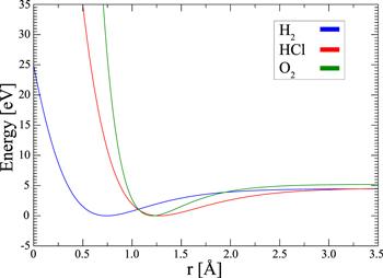
Spectroscopic parameters of the diatomic molecules H2, HCl and O2 are given in table 1, which are taken from [88, 89]. Based on the experimental values such as the dissociation energy De, the equilibrium bond length re, and the equilibrium vibrational frequency νe, the potential parameters V1, V2, V3 and the screening parameter α can be defined by using the expressions (S19), (S20), (S24), and (S28) in4.
Table 1. Spectroscopic molecular parameters for H2, HCl, O2 diatomic molecules. |
| Molecule | μ | re | De | νe |
|---|---|---|---|---|
| (a. m. u. ) | (Å) | (cm−1) | (cm−1) | |
| H2 | 0.5041 | 0.7417 | 36 118.062 | 4395.2 |
| HCl | 0.9799 | 1.274 563 03 | 37 243 | 2990.875 |
| O2 | 8.000 | 1.207 5358 | 42 047 | 1580.194 |
By using these parameters, we present the potential energy curves calculated for H2, HCl, O2 diatomic molecules, see figure 1. Further, we can easily calculate the bound state energy eigenvalues for the diatomic molecules H2, HCl, O2 at n and l quantum states by using the ${E}_{{nl}}^{{NR}}$ expressions of the Schrödinger molecule and ${E}_{{nl}}^{b}={E}_{{nl}}^{R}-{{Mc}}^{2}$ expression of the binding energies KG molecule [2], see table 2. The obtained eigenvalues of the HCl diatomic molecule are in good agreement with experimentally reported values in [90].
Figure 1. Potential energy curves of the diatomic molecules H2, HCl and O2 as a function of the interatomic distance. |
Table 2. The bound state energy eigenvalues ${E}_{{nl}}^{{NR}}$ of the Schrödinger molecule and ${E}_{{nl}}^{b}={E}_{{nl}}^{R}-{{Mc}}^{2}$ of the Klein–Gordon molecule in the GTHP calculated using equation ( |
| n | l | ${E}_{{nl}}^{{NR}},({{\rm{H}}}_{2})$ | ${E}_{{nl}}^{b},({{\rm{H}}}_{2})$ | ${E}_{{nl}}^{{NR}},(\mathrm{HCl})$ | ${E}_{{nl}}^{b},(\mathrm{HCl})$ | ${E}_{{nl}}^{{NR}},({{\rm{O}}}_{2})$ | ${E}_{{nl}}^{b},({{\rm{O}}}_{2})$ |
|---|---|---|---|---|---|---|---|
| (cm−1) | (cm−1) | (cm−1) | (cm−1) | (cm−1) | (cm−1) | ||
| 0 | 0 | 2163.332 479 | 2163.332 477 | 1480.444 771 | 1480.444 675 | 786.437 8165 | 786.437 6894 |
| 1 | 0 | 6327.103 462 | 6327.103 410 | 4359.482 381 | 4359.482 341 | 2338.054 436 | 2338.054 024 |
| 1 | 1 | 6444.845 686 | 6444.845 634 | 4379.847 347 | 4379.847 337 | 2340.894 357 | 2340.894 427 |
| 2 | 0 | 10 252.927 23 | 10 252.927 26 | 7125.499 716 | 7125.499 649 | 3860.922 397 | 3860.922 186 |
| 2 | 1 | 10 367.885 83 | 10 367.885 90 | 7145.313 357 | 7145.313 215 | 3863.729 451 | 3863.729 320 |
| 2 | 2 | 10 596.757 12 | 10 596.757 28 | 7184.927 896 | 7184.927 714 | 3869.343 429 | 3869.344 512 |
| 3 | 0 | 13 934.324 20 | 13 934.324 17 | 9777.517 902 | 9777.517 934 | 5354.985 484 | 5354.985 616 |
| 3 | 1 | 14 046.229 51 | 14 046.229 52 | 9796.773 872 | 9796.773 864 | 5357.759 581 | 5357.759 412 |
| 3 | 2 | 14 269.024 31 | 14 269.024 47 | 9835.273 336 | 9835.273 166 | 5363.306 888 | 5363.307 911 |
| 3 | 3 | 14 600.720 22 | 14 600.720 31 | 9892.991 022 | 9892.990 941 | 5371.629 453 | 5371.630 377 |
| 4 | 0 | 17 364.449 80 | 17 364.449 77 | 12 314.543 22 | 12 314.543 18 | 6820.187 243 | 6820.187 560 |
| 4 | 1 | 17 473.029 85 | 17 473.029 83 | 12 333.235 31 | 12 333.235 23 | 6822.927 545 | 6822.927 953 |
| 4 | 2 | 17 689.208 23 | 17 689.208 38 | 12 370.607 07 | 12 370.606 85 | 6828.408 793 | 6828.409 623 |
| 4 | 3 | 18 011.064 17 | 18 011.064 30 | 12 426.633 34 | 12 426.633 29 | 6836.630 730 | 6836.631 845 |
| 4 | 4 | 18 435.819 49 | 18 435.819 57 | 12 501.277 34 | 12 501.277 24 | 6847.592 259 | 6847.593 247 |
| 5 | 0 | 20 536.070 41 | 20 536.070 39 | 14 735.565 70 | 14 735.565 70 | 8256.471 021 | 8256.471 069 |
| 5 | 1 | 20 641.051 30 | 20 641.051 28 | 14 753.687 76 | 14 753.687 60 | 8259.177 484 | 8259.177 992 |
| 5 | 2 | 20 850.069 73 | 20 850.069 82 | 14 789.919 18 | 14 789.918 98 | 8264.591 767 | 8264.592 703 |
| 5 | 3 | 21 161.280 64 | 21 161.280 76 | 14 844.235 14 | 14 844.235 24 | 8272.713 618 | 8272.714 473 |
| 5 | 4 | 21 572.017 81 | 21 572.017 97 | 14 916.599 24 | 14 916.599 34 | 8283.541 215 | 8283.541 974 |
| 5 | 5 | 22 078.906 37 | 22 078.906 53 | 15 006.962 14 | 15 006.962 07 | 8297.076 277 | 8297.076 196 |
| 6 | 0 | 23 441.536 12 | 23 441.536 08 | 17 039.560 05 | 17 039.559 91 | 9663.779 212 | 9663.779 010 |
| 6 | 1 | 23 542.642 61 | 23 542.642 54 | 17 057.105 39 | 17 057.105 32 | 9666.452 501 | 9666.452 396 |
| 6 | 2 | 23 743.954 74 | 23 743.954 88 | 17 092.184 01 | 17 092.183 82 | 9671.798 959 | 9671.800 000 |
| 6 | 3 | 24 043.712 12 | 24 043.712 23 | 17 144.770 88 | 17 144.770 97 | 9679.820 497 | 9679.821 126 |
| 6 | 4 | 24 439.372 71 | 24 439.372 81 | 17 214.829 91 | 17 214.829 95 | 9690.513 889 | 9690.514 445 |
| 6 | 5 | 24 927.723 10 | 24 927.723 19 | 17 302.311 92 | 17 302.311 89 | 9703.880 795 | 9703.880 933 |
| 6 | 6 | 25 505.011 24 | 25 505.011 31 | 17 407.155 87 | 17 407.155 76 | 9719.918 459 | 9719.919 524 |
While we compare the lowest excitation energies for diatomic molecules, the obtained results are in perfect agreement with the sophisticated high-resolution measurements, see table 3. Although the six parameters Lennard–Jones potential model is a little bit more accurate than GTHP, the fact that GTHP has four parameters is a great advantage for easier modelling of physical systems. Generally, the obtained results allow one to tune and optime the potential concerning its desired properties in atomic, molecular, chemical, condensed matter and high energy physics applications.
Table 3. The lowest rotational △E(l) and vibrational △E(n) excitation energies, all values in cm−1. |
| Molecule | H2 | H2 | HCl | HCl | O2 | O2 |
|---|---|---|---|---|---|---|
| Exc. type | l = 0 → 1 | n = 0 → 1 | l = 0 → 1 | n = 0 → 1 | l = 0 → 1 | n = 0 → 1 |
| Theorya | 117.742 224 | 4163.770 983 | 20.364 966 | 2879.037 610 | 2.839 921 | 1551.616 620 |
| Theoryb | 117.742 224 | 4163.770 933 | 20.364 996 | 2879.037 666 | 2.840 403 | 1551.616 335 |
| Theoryc | ⋯ | ⋯ | ⋯ | 2885.86 | ⋯ | ⋯ |
| Theoryd | ⋯ | ⋯ | ⋯ | 2872.98 | ⋯ | ⋯ |
| Theorye | 118.486 812(9) | 4161.1661(9) | ⋯ | ⋯ | ⋯ | ⋯ |
| $\mathrm{Exp}.$ | 118.486 84(10)f | 4161.1660(03)g, | ||||
| ⋯ | 4161.16632(18)h | ⋯ | 2885.98i |
aThis work for non-relativistic case. | |
bThis work for relativistic case. | |
cAnalytical calculation by extended Lennard-Jones potential, see [89]. | |
dCalculation by ab initio multi-reference configuration interaction calculation with the digit standing for diatomics (EHFACE2), see [90]. | |
eCalculation by nonadiabatic perturbation theory with considering relativistic quantum electrodynamic, see [91]; the experimental value: | |
fSee [92]. | |
gSee [93]. | |
hSee [94]. | |
iSee [90]. |
4. Concluding remarks
In this study, we proposed a new potential model, which holds numerous important physical potentials. Next, the bound state solution of the radial KG equation with this potential is examined analytically within the framework of the NU method. It is also presented that the energy eigenvalues are sensitively associated with potential parameters for quantum states. GTHP and its obtained energy eigenvalues are in remarkable overlap with the reported results in some cases, so this potential model is a desirable candidate for displaying multiple quantum systems concurrently. For more specific cases, GTHP was used to study for modelling several diatomic molecules, and the study showed that the good agreement between the lowest rotational △E(l) and vibrational △E(n) excitation energies and the experimental of H2, HCl and O2 diatomic molecules. In view of the simplicity and accuracy, our work provides additional physical insights about the systems and sheds some light on this potential’s representative power.