


1. Introduction
A higher order nonlinear Schrödinger (NLS) equation1 ) is not integrable. But when choosing some appropriate parameters, it can be shown that equation (1 ) is integrable by inverse scattering transform. Equation (1 ) can be converted to several integrable equations, such as the derivative NLS equation, the Hirota equation and the Sasa-Satsuma equation [3–6].
$\begin{eqnarray}\begin{array}{l}{\rm{i}}{q}_{T}+\displaystyle \frac{1}{2}{q}_{{XX}}+| q{| }^{2}q+{\rm{i}}\epsilon \left({\beta }_{1}{q}_{{XXX}}\right.\\ \quad \left.+{\beta }_{2}| q{| }^{2}{q}_{X}+{\beta }_{3}q{\left(| q{| }^{2}\right)}_{X}\right)=0\end{array}\end{eqnarray}$
was proposed by Kodama and Hasegawa [1, 2], where βj are real constants, and ε is a small parameter. It is originally presented as a model for the femtosecond pulse propagation in a monomode fiber. In the general case, equation (Let us write the Sasa-Satsuma equation2 ) changes into a complex modified KdV-type equation4 ) has been extensively studied by different methods, such as inverse scattering transform [7, 8], Darboux transformation [9–14] and Hirota bilinear method [15, 16].
$\begin{eqnarray}{\rm{i}}{q}_{T}+\displaystyle \frac{1}{2}{q}_{{XX}}+| q{| }^{2}q+{\rm{i}}\left({q}_{{XXX}}+6| q{| }^{2}{q}_{X}+3q{\left(| q{| }^{2}\right)}_{X}\right)=0.\end{eqnarray}$
By introducing variable transformations $\begin{eqnarray}\begin{array}{rcl}u(x,t) & = & q(X,T)\exp \left\{\displaystyle \frac{-{\rm{i}}}{6}\left(X-\displaystyle \frac{T}{18}\right)\right\},\\ t & = & T,\,\,\,x\,=\,X-\displaystyle \frac{T}{12},\end{array}\end{eqnarray}$
Equation ( $\begin{eqnarray}{u}_{t}+{u}_{{xxx}}+6| u{| }^{2}{u}_{x}+3u{\left(| u{| }^{2}\right)}_{x}=0,\end{eqnarray}$
which is also called a Sasa-Satsuma equation. Equation (Based on equation (4 ), a two-component Sasa-Satsuma equation is proposed in [17, 18],5 ) are obtained by Darboux transformation and the Riemann-Hilbert approach.
$\begin{eqnarray}\begin{array}{rcl}{u}_{t} & = & {u}_{{xxx}}+6| u{| }^{2}{u}_{x}+3u{\left(| u{| }^{2}\right)}_{x}+3v{\left({uv}\right)}_{x},\\ {v}_{t} & = & {v}_{{xxx}}+6| u{| }^{2}{v}_{x}+3v{\left(| u{| }^{2}\right)}_{x}+3v{\left({v}^{2}\right)}_{x}.\end{array}\end{eqnarray}$
Soliton solutions of equation (In this paper, inspired by equation (5 ), we introduce a two-component generalized Sasa-Satsuma (gSS) equation6 ), v(x, t) can be either a complex function or a real function. If the reduction is taken as $v={\rm{i}}\sqrt{{b}^{* }}u$, then equation (6 ) changes to7 ) is a gSS equation. We thus can see that it is interesting to study the equation (6 ). It is obvious that when b = 0, the equation (6 ) is reduced to equation (5 ).
$\begin{eqnarray}\begin{array}{rcl}{u}_{t} & = & {u}_{{xxx}}-6a| u{| }^{2}{u}_{x}-3{au}{\left(| u{| }^{2}\right)}_{x}\\ & & -3{{bu}}^{* }{\left(| u{| }^{2}\right)}_{x}-3{b}^{* }u{\left({u}^{2}\right)}_{x}+3v{\left({uv}\right)}_{x},\\ {v}_{t} & = & {v}_{{xxx}}-6a| u{| }^{2}{v}_{x}-3{av}{\left(| u{| }^{2}\right)}_{x}\\ & & -3{{bu}}^{* }{\left({{vu}}^{* }\right)}_{x}-3{b}^{* }u{\left({vu}\right)}_{x}+3v{\left({v}^{2}\right)}_{x},\end{array}\end{eqnarray}$
where u(x, t) is a complex function, a is a real constant, b is a complex constant, and * denotes the complex conjugate. In equation ( $\begin{eqnarray}\begin{array}{rcl}{u}_{t} & = & {u}_{{xxx}}-6a| u{| }^{2}{u}_{x}-3{au}{\left(| u{| }^{2}\right)}_{x}-3{{bu}}^{* }{\left(| u{| }^{2}\right)}_{x}\\ & & -6{b}^{* }u{\left({u}^{2}\right)}_{x}.\end{array}\end{eqnarray}$
Equation (In this paper, we will show that the two-component gSS equation (6 ) is Lax integrable. We will construct its n-fold Darboux transformation. Soliton solutions including a breather soliton solution, kink solution and periodic-like solution will also be constructed.
2. Lax pair for the two-component gSS equation
In this section, we give the following Lax pair of equation (6 ):6 ).
$\begin{eqnarray}\begin{array}{rcl}{{\rm{\Phi }}}_{x} & = & U{\rm{\Phi }}=\left(-{\rm{i}}\lambda \sigma +Q\right){\rm{\Phi }},\\ {{\rm{\Phi }}}_{t} & = & V{\rm{\Phi }}=\left(4{\rm{i}}{\lambda }^{3}\sigma -4{\lambda }^{2}Q+2{\rm{i}}\lambda \left({Q}_{x}+{Q}^{2}\right)\sigma \right.\\ & & \left.+{Q}_{{xx}}-2{Q}^{3}-{Q}_{x}Q+{{QQ}}_{x}\right){\rm{\Phi }},\end{array}\end{eqnarray}$
where $\begin{eqnarray}\begin{array}{rcl}Q & = & \left(\begin{array}{cccc}0 & {au}+{{bu}}^{* } & {{au}}^{* }+{b}^{* }u & -v\\ {u}^{* } & 0 & 0 & 0\\ u & 0 & 0 & 0\\ v & 0 & 0 & 0\end{array}\right),\\ \sigma & = & \left(\begin{array}{cccc}-1 & 0 & 0 & 0\\ 0 & 1 & 0 & 0\\ 0 & 0 & 1 & 0\\ 0 & 0 & 0 & 1\end{array}\right).\end{array}\end{eqnarray}$
It can directly verify that the zero-curvature equation Ut − Vx + [U, V] = 0 yields the two-component gSS equation (We take ${\rm{\Phi }}={\left({\phi }_{1},{\phi }_{2},{\phi }_{3},{\phi }_{4}\right)}^{T}$ is an eigenfunction of Lax pair (8 ) at λ. Note that ${\rm{\Psi }}={\left({\phi }_{1}^{* },{\phi }_{3}^{* },{\phi }_{2}^{* },{\phi }_{4}^{* }\right)}^{T}$ is an eigenfunction of Lax pair (8 ) at −λ* if v is a real function. Thus we can construct the matrix solution of Lax pair (8 )
$\begin{eqnarray}\begin{array}{rcl}{\theta }_{x} & = & -{\rm{i}}\sigma \theta {\rm{\Lambda }}+Q\theta ,\\ {\theta }_{t} & = & 4{\rm{i}}\sigma \theta {{\rm{\Lambda }}}^{3}-4Q\theta {{\rm{\Lambda }}}^{2}+2{\rm{i}}\left({Q}_{x}+{Q}^{2}\right)\sigma \theta {\rm{\Lambda }}\\ & & +\left({Q}_{{xx}}-2{Q}^{3}-{Q}_{x}Q+{{QQ}}_{x}\right)\theta ,\end{array}\end{eqnarray}$
where $\begin{eqnarray}\theta =({\rm{\Phi }},{\rm{\Psi }})=\left(\begin{array}{cc}{\phi }_{1} & {\phi }_{1}^{* }\\ {\phi }_{2} & {\phi }_{3}^{* }\\ {\phi }_{3} & {\phi }_{2}^{* }\\ {\phi }_{4} & {\phi }_{4}^{* }\end{array}\right),\,\,\,\,\,\,\,{\rm{\Lambda }}=\left(\begin{array}{cc}\lambda & 0\\ 0 & -{\lambda }^{* }\end{array}\right).\end{eqnarray}$
3. Darboux transformation of the two-component gSS equation
In this section, we construct the Darboux transformation to the two-component gSS equation (6 ). Firstly, the adjoint problem of Lax pair (8 ) is8 ) at λ = λ1, we can verify that ${\theta }_{1}^{\dagger }(x,t)M$ is an eigenfunction of equation (12 ) at $\lambda =-{\lambda }_{1}^{* }$, where14 ) linear spectral equation (8 ) changes to
$\begin{eqnarray}{{\rm{\Xi }}}_{x}=-{\rm{\Xi }}U,\,\,\,\,\,\,\,\,{{\rm{\Xi }}}_{t}=-{\rm{\Xi }}V.\end{eqnarray}$
Assuming that θ1(x, t) is an eigenfunction of the Lax pair ( $\begin{eqnarray}M=\left(\begin{array}{cccc}-1 & 0 & 0 & 0\\ 0 & a & {b}^{* } & 0\\ 0 & b & a & 0\\ 0 & 0 & 0 & -1\end{array}\right).\end{eqnarray}$
Based on the [9–12], we take the transformation $\begin{eqnarray}{\rm{\Phi }}[1]=T{\rm{\Phi }},\end{eqnarray}$
where $\begin{eqnarray}T\,=\,I-{\theta }_{1}{\rm{\Omega }}{\left({\theta }_{1},{\theta }_{1}\right)}^{-1}{\left(\lambda I-{{\rm{\Lambda }}}^{* }\right)}^{-1}{\theta }_{1}^{\dagger }M,\end{eqnarray}$
with $\begin{eqnarray}\begin{array}{rcl}{\rm{\Omega }}\left({\theta }_{1},{\theta }_{1}\right) & = & \left(\begin{array}{cc}\displaystyle \frac{{{\rm{\Phi }}}_{1}^{\dagger }M{{\rm{\Phi }}}_{1}}{{\lambda }_{1}-{\lambda }_{1}^{* }} & \displaystyle \frac{{{\rm{\Phi }}}_{1}^{\dagger }M{{\rm{\Psi }}}_{1}}{-2{\lambda }_{1}^{* }}\\ \displaystyle \frac{{{\rm{\Psi }}}_{1}^{\dagger }M{{\rm{\Phi }}}_{1}}{2{\lambda }_{1}} & \displaystyle \frac{{{\rm{\Psi }}}_{1}^{\dagger }M{{\rm{\Psi }}}_{1}}{{\lambda }_{1}-{\lambda }_{1}^{* }}\end{array}\right),\\ {{\rm{\Phi }}}^{\dagger } & = & ({\phi }_{1}^{* },{\phi }_{2}^{* },{\phi }_{3}^{* },{\phi }_{4}^{* }),\,\,\,\,{{\rm{\Psi }}}^{\dagger }=({\phi }_{1},{\phi }_{3},{\phi }_{2},{\phi }_{4}).\end{array}\end{eqnarray}$
It is obvious that under the transformation ( $\begin{eqnarray}{\rm{\Phi }}{\left[1\right]}_{x}=U[1]{\rm{\Phi }}[1],\,\,\,\,\,\,\,\,{\rm{\Phi }}{\left[1\right]}_{t}=V[1]{\rm{\Phi }}[1],\end{eqnarray}$
where $\begin{eqnarray}U[1]=\left({T}_{x}+{TU}\right){T}^{-1},\,\,\,\,V[1]=\left({T}_{t}+{TV}\right){T}^{-1}.\end{eqnarray}$
We can show the matrix U[1] and V[1] have the same structures with the matrix U and V, that is $\begin{eqnarray}\begin{array}{rcl}U[1] & = & -{\rm{i}}\lambda \sigma +Q[1],\\ V[1] & = & 4{\rm{i}}{\lambda }^{3}\sigma -4{\lambda }^{2}Q[1]+2{\rm{i}}\lambda \left(Q{\left[1\right]}_{x}+Q{\left[1\right]}^{2}\right)\sigma \\ & & +Q{\left[1\right]}_{{xx}}-2Q{\left[1\right]}^{3}-Q{\left[1\right]}_{x}Q[1]+Q[1]Q{\left[1\right]}_{x},\end{array}\end{eqnarray}$
where the relation between the new potential and the old one is $\begin{eqnarray}Q[1]=Q+{\rm{i}}\left[{\theta }_{1}{\rm{\Omega }}{\left({\theta }_{1},{\theta }_{1}\right)}^{-1}{\theta }_{1}^{\dagger }M,\sigma \right].\end{eqnarray}$
Let us show the conclusion that the matrix U[1] and V[1] have the same structure as the matrix U and V. The matrix T can be rewritten as27 ) into equation (25 ), we obtain26 ) holds. We have the following equations:20 ). By substituting equation (31 ) into the coefficients of λ3, λ2, we can know that the coefficients of λ3, λ2 are zero. From the coefficients of λ3 we can know the representation of S3[1]. Substituting the S3[1] into the coefficients of λ1, λ0, and with the help of maple, we can verify that the coefficients of λ1, λ0 are also zero.
$\begin{eqnarray}\begin{array}{rcl}T & = & I-\displaystyle \frac{1}{{X}_{11}^{2}+| {Y}_{11}{| }^{2}}\left(\displaystyle \frac{\left({X}_{11}{{\rm{\Phi }}}_{1}-{Y}_{11}{{\rm{\Psi }}}_{1}\right){{\rm{\Phi }}}_{1}^{\dagger }M}{\lambda -{\lambda }_{1}^{* }}\right.\\ & & \left.+\displaystyle \frac{\left({Y}_{11}^{* }{{\rm{\Phi }}}_{1}+{X}_{11}{{\rm{\Psi }}}_{1}\right){{\rm{\Psi }}}_{1}^{\dagger }M}{\lambda +{\lambda }_{1}}\right),\end{array}\end{eqnarray}$
where the functions ${X}_{11}=\tfrac{{{\rm{\Phi }}}_{1}^{\dagger }M{{\rm{\Phi }}}_{1}}{{\lambda }_{1}-{\lambda }_{1}^{* }},{Y}_{11}=\tfrac{{{\rm{\Psi }}}_{1}^{\dagger }M{{\rm{\Phi }}}_{1}}{2{\lambda }_{1}}$ . We rewrite the last equation as $\begin{eqnarray}\begin{array}{l}\left(\lambda +{\lambda }_{1}\right)\left(\lambda -{\lambda }_{1}^{* }\right)T=\left(\lambda +{\lambda }_{1}\right)\left(\lambda -{\lambda }_{1}^{* }\right)I\\ \quad -\displaystyle \frac{1}{{X}_{11}^{2}+| {Y}_{11}{| }^{2}}\left(\lambda {S}_{1}+{S}_{2}\right),\end{array}\end{eqnarray}$
where $\begin{eqnarray}{S}_{1}=\left({X}_{11}{{\rm{\Phi }}}_{1}-{Y}_{11}{{\rm{\Psi }}}_{1}\right){{\rm{\Phi }}}_{1}^{\dagger }M+\left({Y}_{11}^{* }{{\rm{\Phi }}}_{1}+{X}_{11}{{\rm{\Psi }}}_{1}\right){{\rm{\Psi }}}_{1}^{\dagger }M,\end{eqnarray}$
$\begin{eqnarray}{S}_{2}={\lambda }_{1}\left({X}_{11}{{\rm{\Phi }}}_{1}-{Y}_{11}{{\rm{\Psi }}}_{1}\right){{\rm{\Phi }}}_{1}^{\dagger }M-{\lambda }_{1}^{* }\left({Y}_{11}^{* }{{\rm{\Phi }}}_{1}+{X}_{11}{{\rm{\Psi }}}_{1}\right){{\rm{\Psi }}}_{1}^{\dagger }M.\end{eqnarray}$
We hope to check that the following equations hold $\begin{eqnarray}\begin{array}{l}\left(\lambda +{\lambda }_{1}\right)\left(\lambda -{\lambda }_{1}^{* }\right){T}_{x}+\left(\lambda +{\lambda }_{1}\right)\left(\lambda -{\lambda }_{1}^{* }\right){TU}\\ \quad =\left(\lambda +{\lambda }_{1}\right)\left(\lambda -{\lambda }_{1}^{* }\right)U[1]T,\end{array}\end{eqnarray}$
$\begin{eqnarray}\begin{array}{l}\left(\lambda +{\lambda }_{1}\right)\left(\lambda -{\lambda }_{1}^{* }\right){T}_{t}+\left(\lambda +{\lambda }_{1}\right)\left(\lambda -{\lambda }_{1}^{* }\right){TV}\\ \quad =\left(\lambda +{\lambda }_{1}\right)\left(\lambda -{\lambda }_{1}^{* }\right)V[1]T.\end{array}\end{eqnarray}$
Supposing $\begin{eqnarray}U[1]={\left({u}_{{ij}}\right)}_{4\,\times \,4},\end{eqnarray}$
and substituting equation ( $\begin{eqnarray*}\begin{array}{rcl}{u}_{14} & = & -v[1],\,\,{u}_{21}={u}^{* }[1],\,\,{u}_{31}=u[1],\,\,{u}_{41}=v[1],\\ {u}_{12} & = & {au}[1]+{{bu}}^{* }[1],{u}_{13}={{au}}^{* }[1]+{b}^{* }u[1],\\ {u}_{11} & = & {\rm{i}}\lambda ,\,\,{u}_{22}={u}_{33}={u}_{44}=-{\rm{i}}\lambda ,\\ {u}_{23} & = & {u}_{24}={u}_{32}={u}_{34}={u}_{42}={u}_{43}=0,\end{array}\end{eqnarray*}$
where $\begin{eqnarray}\begin{array}{l}u[1]=u-\displaystyle \frac{2{\rm{i}}}{{X}_{11}^{2}+| {Y}_{11}{| }^{2}}\left[-{X}_{11}\left({\phi }_{3}{\phi }_{1}^{* }+{\phi }_{1}{\phi }_{2}^{* }\right)\right.\\ \quad \left.+{Y}_{11}{\phi }_{1}^{* }{\phi }_{2}^{* }-{Y}_{11}^{* }{\phi }_{1}{\phi }_{3}\right],\end{array}\end{eqnarray}$
$\begin{eqnarray}\begin{array}{l}v[1]=v-\displaystyle \frac{2{\rm{i}}}{{X}_{11}^{2}+| {Y}_{11}{| }^{2}}\left[-{X}_{11}\left({\phi }_{1}{\phi }_{4}^{* }+{\phi }_{4}{\phi }_{1}^{* }\right)\right.\\ \quad \left.+{Y}_{11}{\phi }_{1}^{* }{\phi }_{4}^{* }-{Y}_{11}^{* }{\phi }_{1}{\phi }_{4}\right].\end{array}\end{eqnarray}$
Thus matrices U[1] and U have the same structures. Since the structure of V[1] is too complex, we directly show the equation ( $\begin{eqnarray*}\begin{array}{l}{\lambda }^{4}:\qquad Q+\displaystyle \frac{{\rm{i}}{S}_{1}\sigma }{{X}_{11}^{2}+| {Y}_{11}{| }^{2}}=Q[1]+\displaystyle \frac{{\rm{i}}\sigma {S}_{1}}{{X}_{11}^{2}+| {Y}_{11}{| }^{2}},\\ {\lambda }^{3}:\qquad 2{\rm{i}}\left({Q}_{x}+{Q}^{2}\right)\sigma -4\left({\lambda }_{1}-{\lambda }_{1}^{* }\right)Q\\ \quad -\displaystyle \frac{\left(-4{S}_{1}Q+4{\rm{i}}{S}_{2}\sigma \right)}{{X}_{11}^{2}+| {Y}_{11}{| }^{2}}\\ \quad =2{\rm{i}}\left(Q{\left[1\right]}_{x}+Q{\left[1\right]}^{2}\right)\sigma -4\left({\lambda }_{1}-{\lambda }_{1}^{* }\right)Q[1]\\ \quad -\displaystyle \frac{\left(-4Q[1]{S}_{1}+4{\rm{i}}\sigma {S}_{2}\right)}{{X}_{11}^{2}+| {Y}_{11}{| }^{2}},\\ {\lambda }^{2}:\qquad {S}_{3}+2{\rm{i}}\left({\lambda }_{1}-{\lambda }_{1}^{* }\right)\left({Q}_{x}+{Q}^{2}\right)\sigma +4{\lambda }_{1}{\lambda }_{1}^{* }Q\\ \quad +\displaystyle \frac{\left(4{S}_{2}Q-2{\rm{i}}{S}_{1}\left({Q}_{x}+{Q}^{2}\right)\sigma \right)}{{X}_{11}^{2}+| {Y}_{11}{| }^{2}}\\ \quad ={S}_{3}[1]+2{\rm{i}}\left({\lambda }_{1}-{\lambda }_{1}^{* }\right)\left(Q{\left[1\right]}_{x}+Q{\left[1\right]}^{2}\right)\sigma +4{\lambda }_{1}{\lambda }_{1}^{* }Q[1]\\ \quad +\displaystyle \frac{\left(4Q[1]{S}_{2}-2{\rm{i}}\left(Q{\left[1\right]}_{x}+Q{\left[1\right]}^{2}\right)\sigma {S}_{1}\right)}{{X}_{11}^{2}+| {Y}_{11}{| }^{2}},\\ {\lambda }^{1}:\qquad -\displaystyle \frac{{S}_{1,t}\left({X}_{11}^{2}+| {Y}_{11}{| }^{2}\right)-{S}_{1}{\left({X}_{11}^{2}+| {Y}_{11}{| }^{2}\right)}_{t}}{{\left({X}_{11}^{2}+| {Y}_{11}{| }^{2}\right)}^{2}}\\ \quad +\left({\lambda }_{1}-{\lambda }_{1}^{* }\right){S}_{3}-2{\rm{i}}{\lambda }_{1}{\lambda }_{1}^{* }\left({Q}_{x}+{Q}^{2}\right)\sigma \\ \quad -\displaystyle \frac{\left({S}_{1}{S}_{3}+2{\rm{i}}{S}_{2}\left({Q}_{x}+{Q}^{2}\right)\sigma \right)}{{X}_{11}^{2}+| {Y}_{11}{| }^{2}}\\ \quad =\left({\lambda }_{1}-{\lambda }_{1}^{* }\right){S}_{3}[1]-2{\rm{i}}{\lambda }_{1}{\lambda }_{1}^{* }\left(Q{\left[1\right]}_{x}+Q{\left[1\right]}^{2}\right)\sigma \\ \quad -\displaystyle \frac{\left({S}_{3}[1]{S}_{1}+2{\rm{i}}\left(Q{\left[1\right]}_{x}+Q{\left[1\right]}^{2}\right)\sigma {S}_{2}\right)}{{X}_{11}^{2}+| {Y}_{11}{| }^{2}},\\ {\lambda }^{0}:\qquad \displaystyle \frac{{S}_{2,t}\left({X}_{11}^{2}+| {Y}_{11}{| }^{2}\right)-{S}_{2}{\left({X}_{11}^{2}+| {Y}_{11}{| }^{2}\right)}_{t}}{{\left({X}_{11}^{2}+| {Y}_{11}{| }^{2}\right)}^{2}}+{\lambda }_{1}{\lambda }_{1}^{* }{S}_{3}\\ \quad +\displaystyle \frac{{S}_{2}{S}_{3}}{{X}_{11}^{2}+| {Y}_{11}{| }^{2}}={\lambda }_{1}{\lambda }_{1}^{* }{S}_{3}[1]+\displaystyle \frac{{S}_{3}[1]{S}_{2}}{{X}_{11}^{2}+| {Y}_{11}{| }^{2}},\end{array}\end{eqnarray*}$
where $\begin{eqnarray}\begin{array}{rcl}{S}_{3} & = & {Q}_{{xx}}-2{Q}^{3}-{Q}_{x}Q+{{QQ}}_{x},\\ {S}_{3}[1] & = & Q{\left[1\right]}_{{xx}}-2Q{\left[1\right]}^{3}-Q{\left[1\right]}_{x}Q[1]+Q[1]Q{\left[1\right]}_{x}.\end{array}\end{eqnarray}$
According to the coefficient of λ4, we have $\begin{eqnarray}Q[1]=Q+\displaystyle \frac{{\rm{i}}({S}_{1}\sigma -\sigma {S}_{1})}{{X}_{11}^{2}+| {Y}_{11}{| }^{2}},\end{eqnarray}$
which is equivalent to equation (Further, we can derive n-fold DT:
$\begin{eqnarray}{\rm{\Phi }}[n]={\rm{\Phi }}-{\rm{\Theta }}{\rm{\Omega }}{\left({\rm{\Theta }},{\rm{\Theta }}\right)}^{-1}{\rm{\Omega }}({\rm{\Phi }},{\rm{\Theta }}),\end{eqnarray}$
where $\begin{eqnarray}\begin{array}{rcl}{\rm{\Theta }} & = & ({\theta }_{1},{\theta }_{2},\ldots ,{\theta }_{n}),\,\,\,\,\,\,\,{\rm{\Omega }}({\theta }_{j},{\rm{\Phi }})=\left(\begin{array}{c}\displaystyle \frac{{{\rm{\Phi }}}_{j}^{\dagger }M{\rm{\Phi }}}{\lambda -{\lambda }_{j}^{* }}\\ \displaystyle \frac{{{\rm{\Psi }}}_{j}^{\dagger }M{\rm{\Phi }}}{\lambda +{\lambda }_{j}}\end{array}\right),\\ {\rm{\Omega }}({\theta }_{k},{\theta }_{j}) & = & \left(\begin{array}{cc}\displaystyle \frac{{{\rm{\Phi }}}_{j}^{\dagger }M{{\rm{\Phi }}}_{k}}{{\lambda }_{k}-{\lambda }_{j}^{* }} & \displaystyle \frac{{{\rm{\Phi }}}_{j}^{\dagger }M{{\rm{\Psi }}}_{k}}{-{\lambda }_{k}^{* }-{\lambda }_{j}^{* }}\\ \displaystyle \frac{{{\rm{\Psi }}}_{j}^{\dagger }M{{\rm{\Phi }}}_{k}}{{\lambda }_{k}+{\lambda }_{j}} & \displaystyle \frac{{{\rm{\Psi }}}_{j}^{\dagger }M{{\rm{\Psi }}}_{k}}{-{\lambda }_{k}^{* }+{\lambda }_{j}}\end{array}\right),\end{array}\end{eqnarray}$
$\begin{eqnarray}\begin{array}{rcl}{\rm{\Omega }}({\rm{\Phi }},{\rm{\Theta }}) & = & \left(\begin{array}{c}{\rm{\Omega }}({\theta }_{1},{\rm{\Phi }})\\ {\rm{\Omega }}({\theta }_{2},{\rm{\Phi }})\\ \vdots \\ {\rm{\Omega }}({\theta }_{n},{\rm{\Phi }})\end{array}\right),\\ {\rm{\Omega }}({\rm{\Theta }},{\rm{\Theta }}) & = & \left(\begin{array}{cccc}{\rm{\Omega }}({\theta }_{1},{\theta }_{1}) & {\rm{\Omega }}({\theta }_{2},{\theta }_{1}) & \ldots & {\rm{\Omega }}({\theta }_{n},{\theta }_{1})\\ {\rm{\Omega }}({\theta }_{1},{\theta }_{2}) & {\rm{\Omega }}({\theta }_{2},{\theta }_{2}) & \ldots & {\rm{\Omega }}({\theta }_{n},{\theta }_{2})\\ \vdots & \vdots & \vdots & \vdots \\ {\rm{\Omega }}({\theta }_{1},{\theta }_{n}) & {\rm{\Omega }}({\theta }_{2},{\theta }_{n}) & \ldots & {\rm{\Omega }}({\theta }_{n},{\theta }_{n})\end{array}\right),\end{array}\end{eqnarray}$
the relationship between new potential and old one is given by $\begin{eqnarray}Q[n]=Q+{\rm{i}}\left[{\rm{\Theta }}{\rm{\Omega }}{\left({\rm{\Theta }},{\rm{\Theta }}\right)}^{-1}{{\rm{\Theta }}}^{\dagger }M,\sigma \right].\end{eqnarray}$
In fact, we have $\begin{eqnarray*}\begin{array}{l}{\rm{\Phi }}{\left[n\right]}_{x}={{\rm{\Phi }}}_{x}-{{\rm{\Theta }}}_{x}{\rm{\Omega }}{\left({\rm{\Theta }},{\rm{\Theta }}\right)}^{-1}{\rm{\Omega }}({\rm{\Phi }},{\rm{\Theta }})\\ \quad +{\rm{\Theta }}{\rm{\Omega }}{\left({\rm{\Theta }},{\rm{\Theta }}\right)}^{-1}{\rm{\Omega }}{\left({\rm{\Theta }},{\rm{\Theta }}\right)}_{x}{\rm{\Omega }}{\left({\rm{\Theta }},{\rm{\Theta }}\right)}^{-1}{\rm{\Omega }}({\rm{\Phi }},{\rm{\Theta }})\\ \quad -{\rm{\Theta }}{\rm{\Omega }}{\left({\rm{\Theta }},{\rm{\Theta }}\right)}^{-1}{\rm{\Omega }}{\left({\rm{\Phi }},{\rm{\Theta }}\right)}_{x}\\ \quad =\left(-{\rm{i}}\lambda \sigma +Q\right){\rm{\Phi }}-\left(-{\rm{i}}\sigma {\rm{\Theta }}{\rm{\Lambda }}+Q{\rm{\Theta }}\right){\rm{\Omega }}{\left({\rm{\Theta }},{\rm{\Theta }}\right)}^{-1}{\rm{\Omega }}({\rm{\Phi }},{\rm{\Theta }})\\ \quad -{\rm{i}}{\rm{\Theta }}{\rm{\Omega }}{\left({\rm{\Theta }},{\rm{\Theta }}\right)}^{-1}{{\rm{\Theta }}}^{\dagger }M\sigma {\rm{\Theta }}{\rm{\Omega }}{\left({\rm{\Theta }},{\rm{\Theta }}\right)}^{-1}{\rm{\Omega }}({\rm{\Phi }},{\rm{\Theta }})\\ \quad +{\rm{i}}{\rm{\Theta }}{\rm{\Omega }}{\left({\rm{\Theta }},{\rm{\Theta }}\right)}^{-1}{{\rm{\Theta }}}^{\dagger }M\sigma {\rm{\Phi }}\\ \quad =\left(-{\rm{i}}\lambda \sigma +Q\right){\rm{\Phi }}-Q{\rm{\Theta }}{\rm{\Omega }}{\left({\rm{\Theta }},{\rm{\Theta }}\right)}^{-1}{\rm{\Omega }}({\rm{\Phi }},{\rm{\Theta }})\\ \quad -{\rm{i}}{\rm{\Theta }}{\rm{\Omega }}{\left({\rm{\Theta }},{\rm{\Theta }}\right)}^{-1}{{\rm{\Theta }}}^{\dagger }M\sigma {\rm{\Theta }}{\rm{\Omega }}{\left({\rm{\Theta }},{\rm{\Theta }}\right)}^{-1}{\rm{\Omega }}({\rm{\Phi }},{\rm{\Theta }})\\ \quad +{\rm{i}}{\rm{\Theta }}{\rm{\Omega }}{\left({\rm{\Theta }},{\rm{\Theta }}\right)}^{-1}{{\rm{\Theta }}}^{\dagger }M\sigma {\rm{\Phi }}\\ \quad +{\rm{i}}\sigma {\rm{\Theta }}{\rm{\Lambda }}{\rm{\Omega }}{\left({\rm{\Theta }},{\rm{\Theta }}\right)}^{-1}{\rm{\Omega }}({\rm{\Phi }},{\rm{\Theta }})-{\rm{i}}\sigma {\rm{\Theta }}{\rm{\Omega }}{\left({\rm{\Theta }},{\rm{\Theta }}\right)}^{-1}{{\rm{\Theta }}}^{\dagger }M{\rm{\Phi }}\\ \quad +{\rm{i}}\sigma {\rm{\Theta }}{\rm{\Omega }}{\left({\rm{\Theta }},{\rm{\Theta }}\right)}^{-1}(\lambda I-{{\rm{\Lambda }}}^{* }){\rm{\Omega }}({\rm{\Phi }},{\rm{\Theta }})\\ \quad =\left(-{\rm{i}}\lambda \sigma +Q\right){\rm{\Phi }}-Q{\rm{\Theta }}{\rm{\Omega }}{\left({\rm{\Theta }},{\rm{\Theta }}\right)}^{-1}{\rm{\Omega }}({\rm{\Phi }},{\rm{\Theta }})\\ \quad -{\rm{i}}{\rm{\Theta }}{\rm{\Omega }}{\left({\rm{\Theta }},{\rm{\Theta }}\right)}^{-1}{{\rm{\Theta }}}^{\dagger }M\sigma {\rm{\Theta }}{\rm{\Omega }}{\left({\rm{\Theta }},{\rm{\Theta }}\right)}^{-1}{\rm{\Omega }}({\rm{\Phi }},{\rm{\Theta }})\\ \quad +{\rm{i}}{\rm{\Theta }}{\rm{\Omega }}{\left({\rm{\Theta }},{\rm{\Theta }}\right)}^{-1}{{\rm{\Theta }}}^{\dagger }M\sigma {\rm{\Phi }}\\ \quad -{\rm{i}}\sigma {\rm{\Theta }}{\rm{\Omega }}{\left({\rm{\Theta }},{\rm{\Theta }}\right)}^{-1}{{\rm{\Theta }}}^{\dagger }M{\rm{\Phi }}\\ \quad +{\rm{i}}\lambda \sigma {\rm{\Theta }}{\rm{\Omega }}{\left({\rm{\Theta }},{\rm{\Theta }}\right)}^{-1}{\rm{\Omega }}({\rm{\Phi }},{\rm{\Theta }})\\ \quad +{\rm{i}}\sigma {\rm{\Theta }}{\rm{\Lambda }}{\rm{\Omega }}{\left({\rm{\Theta }},{\rm{\Theta }}\right)}^{-1}{\rm{\Omega }}({\rm{\Phi }},{\rm{\Theta }})-{\rm{i}}\sigma {\rm{\Theta }}{\rm{\Omega }}{\left({\rm{\Theta }},{\rm{\Theta }}\right)}^{-1}{{\rm{\Lambda }}}^{* }{\rm{\Omega }}({\rm{\Phi }},{\rm{\Theta }})\end{array}\end{eqnarray*}$
$\begin{eqnarray*}\begin{array}{l}\quad =\left(-{\rm{i}}\lambda \sigma +Q\right){\rm{\Phi }}-(-{\rm{i}}\lambda \sigma +Q){\rm{\Theta }}{\rm{\Omega }}{\left({\rm{\Theta }},{\rm{\Theta }}\right)}^{-1}{\rm{\Omega }}({\rm{\Phi }},{\rm{\Theta }})\\ \quad -{\rm{i}}{\rm{\Theta }}{\rm{\Omega }}{\left({\rm{\Theta }},{\rm{\Theta }}\right)}^{-1}{{\rm{\Theta }}}^{\dagger }M\sigma {\rm{\Theta }}{\rm{\Omega }}{\left({\rm{\Theta }},{\rm{\Theta }}\right)}^{-1}{\rm{\Omega }}({\rm{\Phi }},{\rm{\Theta }})\\ \quad +{\rm{i}}{\rm{\Theta }}{\rm{\Omega }}{\left({\rm{\Theta }},{\rm{\Theta }}\right)}^{-1}{{\rm{\Theta }}}^{\dagger }M\sigma {\rm{\Phi }}-{\rm{i}}\sigma {\rm{\Theta }}{\rm{\Omega }}{\left({\rm{\Theta }},{\rm{\Theta }}\right)}^{-1}{{\rm{\Theta }}}^{\dagger }M{\rm{\Phi }}\\ \quad +{\rm{i}}\sigma {\rm{\Theta }}{\rm{\Omega }}{\left({\rm{\Theta }},{\rm{\Theta }}\right)}^{-1}{{\rm{\Theta }}}^{\dagger }M{\rm{\Theta }}{\rm{\Omega }}{\left({\rm{\Theta }},{\rm{\Theta }}\right)}^{-1}{\rm{\Omega }}({\rm{\Phi }},{\rm{\Theta }})\\ \quad =\left(-{\rm{i}}\lambda \sigma +Q-{\rm{i}}\sigma {\rm{\Theta }}{\rm{\Omega }}{\left({\rm{\Theta }},{\rm{\Theta }}\right)}^{-1}{{\rm{\Theta }}}^{\dagger }M\right.\\ \quad \left.+{\rm{i}}{\rm{\Theta }}{\rm{\Omega }}{\left({\rm{\Theta }},{\rm{\Theta }}\right)}^{-1}{{\rm{\Theta }}}^{\dagger }M\sigma \right)\\ \quad \left({\rm{\Phi }}-{\rm{\Theta }}{\rm{\Omega }}{\left({\rm{\Theta }},{\rm{\Theta }}\right)}^{-1}{\rm{\Omega }}({\rm{\Phi }},{\rm{\Theta }})\right)\\ \quad =\left(-{\rm{i}}\lambda \sigma +Q[n]\right){\rm{\Phi }}[n].\end{array}\end{eqnarray*}$
Here we use the two formulas of Θ†MΦ = (λI − Λ*)ω(Φ, Θ) and Θ†MΘ = ω(Θ, Θ)Λ − Λ*ω(Θ, Θ). Because the computation is too complicated, a detailed proof of ${\rm{\Phi }}{\left[n\right]}_{t}=V[n]{\rm{\Phi }}[n]$ is not given here.4. Soliton solutions of the gSS equation
In this section, we consider different types of soliton solutions of equation (6 ) from zero seed solution and nonzero seed solution, respectively. From equation (20 ) we have
$\begin{eqnarray}\begin{array}{rcl}u[1] & = & u-\displaystyle \frac{2{\rm{i}}}{{X}_{11}^{2}+| {Y}_{11}{| }^{2}}\left[-{X}_{11}\left({\phi }_{3}{\phi }_{1}^{* }+{\phi }_{1}{\phi }_{2}^{* }\right)\right.\\ & & \left.+{Y}_{11}{\phi }_{1}^{* }{\phi }_{2}^{* }-{Y}_{11}^{* }{\phi }_{1}{\phi }_{3}\right],\\ v[1] & = & v-\displaystyle \frac{2{\rm{i}}}{{X}_{11}^{2}+| {Y}_{11}{| }^{2}}\left[-{X}_{11}\left({\phi }_{1}{\phi }_{4}^{* }+{\phi }_{4}{\phi }_{1}^{* }\right)\right.\\ & & \left.+{Y}_{11}{\phi }_{1}^{* }{\phi }_{4}^{* }-{Y}_{11}^{* }{\phi }_{1}{\phi }_{4}\right],\end{array}\end{eqnarray}$
with $\begin{eqnarray}\begin{array}{rcl}{X}_{11} & = & \displaystyle \frac{1}{{\lambda }_{1}-{\lambda }_{1}^{* }}\left[a\left(| {\phi }_{2}{| }^{2}+| {\phi }_{3}{| }^{2}\right)+b{\phi }_{2}{\phi }_{3}^{* }\right.\\ & & \left.+{b}^{* }{\phi }_{3}{\phi }_{2}^{* }-| {\phi }_{1}{| }^{2}-| {\phi }_{4}{| }^{2}\right],\\ {Y}_{11} & = & \displaystyle \frac{1}{2{\lambda }_{1}}\left(2a{\phi }_{2}{\phi }_{3}+b{\phi }_{2}^{2}+{b}^{* }{\phi }_{3}^{2}-{\phi }_{1}^{2}-{\phi }_{4}^{2}\right).\end{array}\end{eqnarray}$
4.1. Soliton solution from zero seed solution
Setting zero seed solutions u = 0, v = 0 of the gSS equation (6 ) and solving the Lax pair (8 ) at λ = λ1, we obtain38 ) into solution (36 ), we obtain39 ) represents the breather solution which is shown in figure 1. When ξ = 0, the breather solution becomes to soliton solution40 ) represent soliton solutions that propagate with the same velocity 4η2. The amplitude of ∣u[1]∣ is $\left|\tfrac{2\eta {\delta }_{1}}{\sqrt{| {\beta }_{1}{\beta }_{2}| }}\right|$ and it is localized at the line $\tfrac{1}{2}\mathrm{ln}\left|\tfrac{{\beta }_{2}}{{\beta }_{1}}\right|+2{\omega }_{1}=0$. The amplitude of v[1] is $\tfrac{2\eta {\delta }_{2}}{\sqrt{| {\beta }_{1}{\beta }_{2}| }}$ and it is localized at the line $\tfrac{1}{2}\mathrm{ln}\left|\tfrac{{\beta }_{2}}{{\beta }_{1}}\right|+2{\omega }_{1}=0$. It should be pointed out that the case of a = b, ck ∈ R(k = 1, 2, 3, 4) cannot appear simultaneously, otherwise the solutions have singularity. Because the plots of ∣u[1]∣ and v[1] are similar, we only exhibit the evolution of soliton solution ∣u[1]∣ given by (40 )in figure 2.
$\begin{eqnarray}\begin{array}{rcl}{{\rm{\Phi }}}_{1} & = & \left({c}_{1}{{\rm{e}}}^{{\rm{i}}{\lambda }_{1}(x-4{\lambda }_{1}^{2}t)},{c}_{2}{{\rm{e}}}^{-{\rm{i}}{\lambda }_{1}(x-4{\lambda }_{1}^{2}t)},{c}_{3}{{\rm{e}}}^{-{\rm{i}}{\lambda }_{1}(x-4{\lambda }_{1}^{2}t)},\right.\\ & & {\left.{c}_{4}{{\rm{e}}}^{-{\rm{i}}{\lambda }_{1}(x-4{\lambda }_{1}^{2}t)}\right)}^{T},\\ {\lambda }_{1} & = & \xi +{\rm{i}}\eta ,\end{array}\end{eqnarray}$
where ck(k = 1, 2, 3, 4) are all complex constants. Substituting the equation ( $\begin{eqnarray}\begin{array}{l}u[1]=\\ -4\eta \displaystyle \frac{{g}_{1}{{\rm{e}}}^{-2{\varsigma }_{1}-2{\rm{i}}{d}_{1}}-{g}_{2}{{\rm{e}}}^{-2{\varsigma }_{1}+2{\rm{i}}{d}_{1}}+{g}_{3}{{\rm{e}}}^{2{\varsigma }_{1}-2{\rm{i}}{d}_{1}}+{g}_{4}{{\rm{e}}}^{2{\varsigma }_{1}+2{\rm{i}}{d}_{1}}}{{f}_{1}{{\rm{e}}}^{-4{\varsigma }_{1}}-{f}_{2}{{\rm{e}}}^{4{\varsigma }_{1}}+{f}_{3}-{\eta }^{2}\left({f}_{4}{{\rm{e}}}^{-4{\rm{i}}{d}_{1}}+{f}_{4}^{* }{{\rm{e}}}^{4{\rm{i}}{d}_{1}}\right)},\\ v[1]=\\ -4\eta \displaystyle \frac{{h}_{1}{{\rm{e}}}^{-2{\varsigma }_{1}-2{\rm{i}}{d}_{1}}+{h}_{1}^{* }{{\rm{e}}}^{-2{\varsigma }_{1}+2{\rm{i}}{d}_{1}}+{h}_{2}{{\rm{e}}}^{2{\varsigma }_{1}-2{\rm{i}}{d}_{1}}+{h}_{2}^{* }{{\rm{e}}}^{2{\varsigma }_{1}+2{\rm{i}}{d}_{1}}}{{f}_{1}{{\rm{e}}}^{-4{\varsigma }_{1}}-{f}_{2}{{\rm{e}}}^{4{\varsigma }_{1}}+{f}_{3}-{\eta }^{2}\left({f}_{4}{{\rm{e}}}^{-4{\rm{i}}{d}_{1}}+{f}_{4}^{* }{{\rm{e}}}^{4{\rm{i}}{d}_{1}}\right)},\end{array}\end{eqnarray}$
where $\begin{eqnarray*}\begin{array}{rcl}{\varsigma }_{1} & = & -\eta x+4\eta \left(3{\xi }^{2}-{\eta }^{2}\right)t,\,\,\,\,\,\,{d}_{1}=\xi x+4\xi \left(3{\eta }^{2}-{\xi }^{2}\right)t,\\ {g}_{1} & = & {\rm{i}}{\alpha }_{2}\eta {c}_{1}^{* }{c}_{2}^{* }(\xi -{\rm{i}}\eta )-{\alpha }_{1}{c}_{3}{c}_{1}^{* }({\xi }^{2}+{\eta }^{2}),\\ {g}_{3} & = & {c}_{3}{c}_{1}{\left({c}_{1}^{* }\right)}^{2}\xi (\xi +{\rm{i}}\eta ),\\ {g}_{2} & = & {\alpha }_{1}{c}_{1}{c}_{2}^{* }({\xi }^{2}+{\eta }^{2})+{\rm{i}}{\alpha }_{2}^{* }\eta (\xi +{\rm{i}}\eta ){c}_{1}{c}_{3},\\ {g}_{4} & = & {c}_{1}^{2}{c}_{1}^{* }{c}_{2}^{* }\xi (\xi -{\rm{i}}\eta ),\\ {h}_{1} & = & {\rm{i}}{\alpha }_{2}{c}_{1}^{* }{c}_{4}^{* }\eta (\xi -{\rm{i}}\eta )-{\alpha }_{1}{c}_{1}^{* }{c}_{4}({\xi }^{2}+{\eta }^{2}),\\ {h}_{2} & = & {\left({c}_{1}^{* }\right)}^{2}{c}_{1}{c}_{4}\xi (\xi +{\rm{i}}\eta ),\\ {f}_{1} & = & {\eta }^{2}| {\alpha }_{2}{| }^{2}-({\xi }^{2}+{\eta }^{2}){\alpha }_{1}^{2},\,\,{f}_{2}={\xi }^{2}| {c}_{1}{| }^{4},\\ {f}_{3} & = & 2{\alpha }_{1}| {c}_{1}{| }^{2}({\xi }^{2}+{\eta }^{2}),\,\,\,{f}_{4}={\alpha }_{2}{\left({c}_{1}^{* }\right)}^{2},\\ {\alpha }_{1} & = & a\left(| {c}_{2}{| }^{2}+| {c}_{3}{| }^{2}\right)+2\mathrm{Re}({{bc}}_{2}{c}_{3}^{* })-| {c}_{4}{| }^{2},\\ {\alpha }_{2} & = & 2{{ac}}_{2}{c}_{3}+{{bc}}_{2}^{2}+{b}^{* }{c}_{3}^{2}-{c}_{4}^{2}.\end{array}\end{eqnarray*}$
Solution ( $\begin{eqnarray}\begin{array}{rcl}u[1] & = & \displaystyle \frac{-2\eta {\delta }_{1}}{\sqrt{| {\beta }_{1}{\beta }_{2}| }}{\rm{sech}} \left(\displaystyle \frac{1}{2}\mathrm{ln}\left|\displaystyle \frac{{\beta }_{2}}{{\beta }_{1}}\right|+2{\omega }_{1}\right),\\ v[1] & = & \displaystyle \frac{-2\eta {\delta }_{2}}{\sqrt{| {\beta }_{1}{\beta }_{2}| }}{\rm{sech}} \left(\displaystyle \frac{1}{2}\mathrm{ln}\left|\displaystyle \frac{{\beta }_{2}}{{\beta }_{1}}\right|+2{\omega }_{1}\right),\end{array}\end{eqnarray}$
where $\begin{eqnarray*}\begin{array}{rcl}{\omega }_{1} & = & -\eta x-4{\eta }^{3}t,\\ {\alpha }_{1} & = & a\left(| {c}_{2}{| }^{2}+| {c}_{3}{| }^{2}\right)+2\mathrm{Re}\left({{bc}}_{2}{c}_{3}^{* }\right)-| {c}_{4}{| }^{2},\\ {\alpha }_{2} & = & 2{{ac}}_{2}{c}_{3}+{{bc}}_{2}^{2}+{b}^{* }{c}_{3}^{2}-{c}_{4}^{2},\\ {\beta }_{1} & = & | {\alpha }_{2}{| }^{2}-{\alpha }_{1}^{2},\,\,\,\,\,{\beta }_{2}=2{\alpha }_{1}| {c}_{1}{| }^{2}-2\mathrm{Re}({\alpha }_{2}^{* }{c}_{1}^{2}),\\ {\delta }_{1} & = & -{\alpha }_{1}\left({c}_{3}{c}_{1}^{* }+{c}_{1}{c}_{2}^{* }\right)+{\alpha }_{2}{c}_{1}^{* }{c}_{2}^{* }+{\alpha }_{2}^{* }{c}_{1}{c}_{3},\\ {\delta }_{2} & = & -2{\alpha }_{1}\mathrm{Re}({c}_{1}{c}_{4}^{* })+2\mathrm{Re}\left({\alpha }_{2}{c}_{1}^{* }{c}_{4}^{* }\right).\end{array}\end{eqnarray*}$
The solutions u[1] and v[1] given by (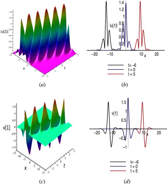
Figure 1. The evolution of the breather solution ( |
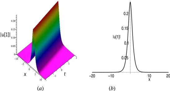
Figure 2. The evolution of the soliton solution ( |
4.2. Soliton solution from nonzero seed solution
Substituting nonzero seed solutions u = s, v = r, where s and r are two constants, into the Lax pair (8 ), we get
$\begin{eqnarray}\begin{array}{rcl}{\phi }_{1} & = & {d}_{3}{{\rm{e}}}^{\tau x\,+\,{mt}}+{d}_{4}{{\rm{e}}}^{-\tau x-{mt}},\\ {\phi }_{2} & = & \left({{as}}^{* }+{b}^{* }s\right){d}_{1}{{\rm{e}}}^{-{\rm{i}}{\lambda }_{1}(x-4{\lambda }_{1}^{2}t)}+\displaystyle \frac{{s}^{* }}{{\rm{i}}{\lambda }_{1}+\tau }{d}_{3}{{\rm{e}}}^{\tau x+{mt}}\\ & & +\displaystyle \frac{{s}^{* }}{{\rm{i}}{\lambda }_{1}-\tau }{d}_{4}{{\rm{e}}}^{-\tau x-{mt}},\\ {\phi }_{3} & = & \left[-\left({as}+{{bs}}^{* }\right){d}_{1}+{{rd}}_{2}\right]{{\rm{e}}}^{-{\rm{i}}{\lambda }_{1}(x-4{\lambda }_{1}^{2}t)}\\ & & +\displaystyle \frac{s}{{\rm{i}}{\lambda }_{1}+\tau }{d}_{3}{{\rm{e}}}^{\tau x\,+\,{mt}}+\displaystyle \frac{s}{{\rm{i}}{\lambda }_{1}-\tau }{d}_{4}{{\rm{e}}}^{-\tau x-{mt}},\\ {\phi }_{4} & = & \left({{as}}^{* }+{b}^{* }s\right){d}_{2}{{\rm{e}}}^{-{\rm{i}}{\lambda }_{1}(x-4{\lambda }_{1}^{2}t)}\\ & & +\displaystyle \frac{r}{{\rm{i}}{\lambda }_{1}+\tau }{d}_{3}{{\rm{e}}}^{\tau x+{mt}}+\displaystyle \frac{r}{{\rm{i}}{\lambda }_{1}-\tau }{d}_{4}{{\rm{e}}}^{-\tau x-{mt}},\end{array}\end{eqnarray}$
where $\begin{eqnarray}\begin{array}{rcl}\tau & = & \sqrt{2a| s{| }^{2}+2\mathrm{Re}({b}^{* }{s}^{2})-{r}^{2}-{\lambda }_{1}^{2}},\\ m & = & -\tau \left[4a| s{| }^{2}+4\mathrm{Re}({b}^{* }{s}^{2})-2{r}^{2}+4{\lambda }_{1}^{2}\right].\end{array}\end{eqnarray}$
Let us consider the following two cases where we set $s=r=1,a=-\tfrac{1}{2}$.Case 1: τ ∈ R, i.e. $2a| s{| }^{2}+2\mathrm{Re}({b}^{* }{s}^{2})-{r}^{2}-{\lambda }_{1}^{2}\gt 0$.
(i) Let ${d}_{3}={d}_{4}=1,{d}_{2}=\tfrac{{\rm{i}}}{2},b=\tfrac{1}{3}$. We have43 ) describes the propagation process of one soliton splitting into two solitons.
$\begin{eqnarray}u[1]=\displaystyle \frac{{K}_{1}}{K},\,\,\,\,\,\,v[1]=\displaystyle \frac{{K}_{2}}{K},\end{eqnarray}$
with $\begin{eqnarray*}\begin{array}{rcl}{K}_{1} & = & -48\sqrt{3}\cosh \left(\displaystyle \frac{1}{2}\mathrm{ln}\left(\displaystyle \frac{3\sqrt{3}+\sqrt{11}}{4}\right)+2{R}_{2}\right)\\ & & +(45+18{\rm{i}}){{\rm{e}}}^{{R}_{1}}\cosh {R}_{2}+\displaystyle \frac{5}{8}{{\rm{e}}}^{2{R}_{1}}-152,\\ {K}_{2} & = & -48\sqrt{3}\cosh \left(\displaystyle \frac{1}{2}\mathrm{ln}\left(\displaystyle \frac{3\sqrt{3}+\sqrt{11}}{4}\right)+2{R}_{2}\right)\\ & & -15{{\rm{e}}}^{2{R}_{1}}\cosh {R}_{2}+\displaystyle \frac{5}{8}{{\rm{e}}}^{2{R}_{1}}-152,\\ K & = & 48\sqrt{3}\cosh \left(\displaystyle \frac{1}{2}\mathrm{ln}\left(\displaystyle \frac{3\sqrt{3}+\sqrt{11}}{4}\right)+2{R}_{2}\right)\\ & & +\displaystyle \frac{5}{8}{{\rm{e}}}^{2{R}_{1}}+64,\end{array}\end{eqnarray*}$
where ${R}_{1}=\tfrac{3}{2}(x+9t),{R}_{2}=\tfrac{\sqrt{33}}{18}(3x+35t)$. We can see from figure 3 that the soliton solution (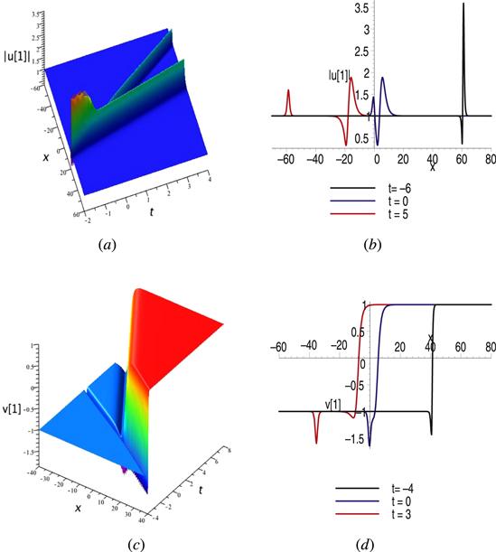
Figure 3. The evolution of the soliton solution ( |
(ii) Let ${d}_{2}=1,{d}_{4}=0,{d}_{3}=\tfrac{{\rm{i}}}{2},b=\tfrac{1}{3}$. We have44 ) is an anti-soliton soliton that propagates along the line $x=\left(\tfrac{3\sqrt{33}-43}{6}\right)t+\tfrac{9+\sqrt{33}}{16}\mathrm{ln}\tfrac{{A}_{2}}{{A}_{3}}$. The solution v[1] is a kink solution (see figure 4(a)-4(b)).
$\begin{eqnarray}\begin{array}{rcl}u[1] & = & \displaystyle \frac{{\rm{i}}{A}_{1}{{\rm{e}}}^{{R}_{2}+{R}_{1}}-{A}_{2}{{\rm{e}}}^{2{R}_{2}}+{A}_{3}{{\rm{e}}}^{2{R}_{1}}}{{A}_{2}{{\rm{e}}}^{2{R}_{2}}+{A}_{3}{{\rm{e}}}^{2{R}_{1}}},\\ v[1] & = & -\tanh \left(\displaystyle \frac{1}{2}\mathrm{ln}\left(\displaystyle \frac{{A}_{2}}{{A}_{3}}\right)+{R}_{2}-{R}_{1}\right),\end{array}\end{eqnarray}$
where $\begin{eqnarray*}\begin{array}{rcl}{A}_{1} & = & 71064-12312\sqrt{33},\,\,\,{A}_{2}=1863\sqrt{33}-10935,\\ {A}_{3} & = & 4560\sqrt{33}-26320.\end{array}\end{eqnarray*}$
The solution ∣u[1]∣ given by (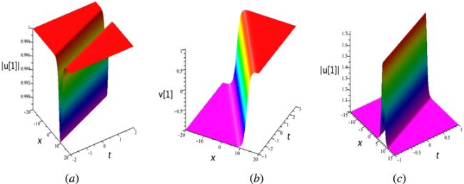
Figure 4. The evolution of solutions ( |
When b = 0, we have45 ) is a soliton solution that propagates along the line $x=-7t+\tfrac{1}{2}\mathrm{ln}\tfrac{3}{4}$ (see figure 4(c)), and v[1] is still a kink solution.
$\begin{eqnarray}\begin{array}{rcl}u[1] & = & \displaystyle \frac{-12{\mathrm{ie}}^{{R}_{3}+{R}_{1}}+4{{\rm{e}}}^{2{R}_{1}}-3{{\rm{e}}}^{2{R}_{3}}}{3{{\rm{e}}}^{2{R}_{3}}+4{{\rm{e}}}^{2{R}_{1}}},\\ v[1] & = & -\tanh \left(\displaystyle \frac{1}{2}\mathrm{ln}\left(\displaystyle \frac{3}{4}\right)+{R}_{3}-{R}_{1}\right),\end{array}\end{eqnarray}$
where ${R}_{3}=\tfrac{1}{2}(x+13t)$. The solution ∣u[1]∣ given by (We note that the solution ∣u[1]∣ given by (44 ) is an anti-soliton solution where b ≠ 0 and the solution ∣u[1]∣ given by (45 ) is a soliton solution where b = 0. This shows that there is a difference between equation (6 ) and equation (5 ).
Case 2: If $2a| s{| }^{2}+2\mathrm{Re}({b}^{* }{s}^{2})-{r}^{2}-{\lambda }_{1}^{2}\lt 0$, $\mathrm{Re}(\tau )=0$, depending on the different choices of d2 and d4, we can obtain the following two solutions.
(i) Let ${d}_{2}=1,{d}_{3}=\tfrac{{\rm{i}}}{2},{d}_{4}=0,b=\tfrac{1}{3}$. We have46 ) is a breather which is shown in figure 5. When t → ± ∞ , ∣u[1]∣ → 1, v[1] → 1.
$\begin{eqnarray}u[1]=1-\displaystyle \frac{{G}_{1}}{G},\,\,\,\,\,\,v[1]=1-\displaystyle \frac{{G}_{2}}{G},\end{eqnarray}$
where $\begin{eqnarray*}\begin{array}{rcl}{G}_{1} & = & 9\left({\sigma }_{1}{{\rm{e}}}^{-2{\rm{i}}{R}_{5}+{R}_{4}}+{\sigma }_{1}^{* }{{\rm{e}}}^{2{\rm{i}}{R}_{5}+{R}_{4}}+{\sigma }_{2}{{\rm{e}}}^{-{\rm{i}}{R}_{5}}+{\sigma }_{3}{{\rm{e}}}^{{\rm{i}}{R}_{5}}\right.\\ & & \left.+1536{\mathrm{ie}}^{-{\rm{i}}{R}_{5}+2{R}_{4}}-1024{\mathrm{ie}}^{{\rm{i}}{R}_{5}+2{R}_{4}}+552{{\rm{e}}}^{{R}_{4}}\right),\\ {G}_{2} & = & 3\left({\omega }_{1}{{\rm{e}}}^{-2{\rm{i}}{R}_{5}+{R}_{4}}+{\omega }_{1}^{* }{{\rm{e}}}^{2{\rm{i}}{R}_{5}+{R}_{4}}-{\omega }_{2}{{\rm{e}}}^{-{\rm{i}}{R}_{5}}\right.\\ & & \left.-{\omega }_{2}^{* }{{\rm{e}}}^{{\rm{i}}{R}_{5}}-2560{{\rm{e}}}^{2{R}_{4}}\sin {R}_{5}+1656{{\rm{e}}}^{{R}_{4}}\right),\\ G & = & {m}_{1}{{\rm{e}}}^{-2{\rm{i}}{R}_{5}+{R}_{4}}+{m}^{* }{{\rm{e}}}^{2{\rm{i}}{R}_{5}+{R}_{4}}+5120{{\rm{e}}}^{3{R}_{4}}\\ & & +13248{{\rm{e}}}^{{R}_{4}}+3159{{\rm{e}}}^{-{R}_{4}},\end{array}\end{eqnarray*}$
with $\begin{eqnarray*}\begin{array}{rcl}{R}_{4} & = & \displaystyle \frac{1}{2}\left(x+t\right),\,\,\,\,\,\,{R}_{5}=\displaystyle \frac{\sqrt{39}}{18}\left(3x+11t\right),\\ {\sigma }_{1} & = & 68{\rm{i}}\sqrt{39}-204,\,\,\,{\sigma }_{2}=819{\rm{i}}-63\sqrt{39},\\ {\sigma }_{3} & = & 9\sqrt{39}+117{\rm{i}},\\ {\omega }_{1} & = & 204{\rm{i}}\sqrt{39}-612,\,\,\,{\omega }_{2}=351{\rm{i}}-27\sqrt{39},\\ {m}_{1} & = & 306{\rm{i}}\sqrt{39}-918.\end{array}\end{eqnarray*}$
The solution (
Figure 5. The evolution of the breather solution ( |
(ii) Let ${d}_{2}=0,{d}_{3}=\tfrac{{\rm{i}}}{2},{d}_{4}=1,b=\tfrac{1}{3}$. We have47 ) is a periodic-like solution, which is a plane on the left and a periodic wave on the right (see figure 6).
$\begin{eqnarray}u[1]=1+\displaystyle \frac{{F}_{1}}{F},\,\,\,\,\,\,v[1]=1+\displaystyle \frac{{F}_{2}}{F},\end{eqnarray}$
where $\begin{eqnarray*}\begin{array}{rcl}{F}_{1} & = & 2\left({\rm{i}}{l}_{1}\cos {R}_{5}-{\rm{i}}{l}_{2}\sin {R}_{5}-{l}_{3}{{\rm{e}}}^{{R}_{4}}\sin 2{R}_{5}\right.\\ & & \left.+{l}_{4}{{\rm{e}}}^{{R}_{4}}\cos 2{R}_{5}+75{{\rm{e}}}^{{R}_{4}}\right).\\ {F}_{2} & = & 2\left(-{l}_{3}\sin 2{R}_{5}+{l}_{4}\cos 2{R}_{5}+75\right),\\ F & = & {l}_{3}{{\rm{e}}}^{{R}_{4}}\sin 2{R}_{5}-{l}_{4}{{\rm{e}}}^{{R}_{4}}\cos 2{R}_{5}-400{{\rm{e}}}^{{R}_{4}}-3159{{\rm{e}}}^{-{R}_{4}},\end{array}\end{eqnarray*}$
with $\begin{eqnarray*}\begin{array}{rcl}{l}_{1} & = & 54\sqrt{39}-351,\,\,\,\,\,\,{l}_{2}=27\sqrt{39}+702,\\ {l}_{3} & = & 15\sqrt{39}+60,\,\,\,\,\,\,\,\,{l}_{4}=45-20\sqrt{39}.\end{array}\end{eqnarray*}$
The solution (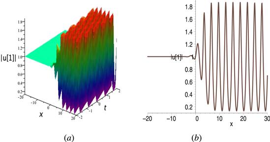
Figure 6. The evolution of periodic-like solution ∣u[1]∣ with parameter: ${\lambda }_{1}=\tfrac{1}{2}{\rm{i}}$. |
5. Two-soliton solutions of the gSS equation
By using the two-fold Darboux transformation, we have37 ).
$\begin{eqnarray}u[2]=u\,+\,2{\rm{i}}\displaystyle \frac{{W}_{1}}{W},\,\,\,\,v[2]=v\,+\,2{\rm{i}}\displaystyle \frac{{W}_{2}}{W},\end{eqnarray}$
where $\begin{eqnarray*}\begin{array}{rcl}W & = & \left|\begin{array}{cccc}{X}_{11} & -{Y}_{11}^{* } & -{X}_{21}^{* } & -{Y}_{21}^{* }\\ {Y}_{11} & {X}_{11} & {Y}_{21} & {X}_{21}\\ {X}_{21} & -{Y}_{21}^{* } & {X}_{22} & -{Y}_{22}^{* }\\ {Y}_{21} & -{X}_{21}^{* } & {Y}_{22} & {X}_{22}\end{array}\right|,\\ {W}_{1} & = & \left|\begin{array}{ccccc}{X}_{11} & -{Y}_{11}^{* } & -{X}_{21}^{* } & -{Y}_{21}^{* } & -{\phi }_{1}^{* }\\ {Y}_{11} & {X}_{11} & {Y}_{21} & {X}_{21} & -{\phi }_{1}\\ {X}_{21} & -{Y}_{21}^{* } & {X}_{22} & -{Y}_{22}^{* } & -{\phi }_{5}^{* }\\ {Y}_{21} & -{X}_{21}^{* } & {Y}_{22} & {X}_{22} & -{\phi }_{5}\\ {\phi }_{3} & {\phi }_{2}^{* } & {\phi }_{7} & {\phi }_{6}^{* } & 0\end{array}\right|,\\ {W}_{2} & = & \left|\begin{array}{ccccc}{X}_{11} & -{Y}_{11}^{* } & -{X}_{21}^{* } & -{Y}_{21}^{* } & -{\phi }_{1}^{* }\\ {Y}_{11} & {X}_{11} & {Y}_{21} & {X}_{21} & -{\phi }_{1}\\ {X}_{21} & -{Y}_{21}^{* } & {X}_{22} & -{Y}_{22}^{* } & -{\phi }_{5}^{* }\\ {Y}_{21} & -{X}_{21}^{* } & {Y}_{22} & {X}_{22} & -{\phi }_{5}\\ {\phi }_{4} & {\phi }_{4}^{* } & {\phi }_{8} & {\phi }_{8}^{* } & 0\end{array}\right|,\end{array}\end{eqnarray*}$
with $\begin{eqnarray*}\begin{array}{rcl}{X}_{21} & = & \displaystyle \frac{1}{{\lambda }_{1}-{\lambda }_{2}^{* }}\left[a\left({\phi }_{3}{\phi }_{7}^{* }+{\phi }_{2}{\phi }_{6}^{* }\right)+b{\phi }_{2}{\phi }_{7}^{* }\right.\\ & & \left.+{b}^{* }{\phi }_{3}{\phi }_{6}^{* }-{\phi }_{1}{\phi }_{5}^{* }-{\phi }_{4}{\phi }_{8}^{* }\right],\\ {Y}_{21} & = & \displaystyle \frac{1}{{\lambda }_{1}+{\lambda }_{2}}\left[a\left({\phi }_{3}{\phi }_{6}+{\phi }_{2}{\phi }_{7}\right)+b{\phi }_{2}{\phi }_{6}\right.\\ & & \left.+{b}^{* }{\phi }_{3}{\phi }_{7}-{\phi }_{1}{\phi }_{5}-{\phi }_{4}{\phi }_{8}\right],\\ {X}_{22} & = & \displaystyle \frac{1}{{\lambda }_{2}-{\lambda }_{2}^{* }}\left[a\left(| {\phi }_{6}{| }^{2}+| {\phi }_{7}{| }^{2}\right)+b{\phi }_{6}{\phi }_{7}^{* }\right.\\ & & \left.+{b}^{* }{\phi }_{7}{\phi }_{6}^{* }-| {\phi }_{5}{| }^{2}-| {\phi }_{8}{| }^{2}\right],\\ {Y}_{22} & = & \displaystyle \frac{1}{2{\lambda }_{2}}\left(2a{\phi }_{6}{\phi }_{7}+b{\phi }_{6}^{2}+{b}^{* }{\phi }_{7}^{2}-{\phi }_{5}^{2}-{\phi }_{8}^{2}\right),\end{array}\end{eqnarray*}$
and X11 and Y11 are represented by equation (5.1. Two-soliton solutions from zero seed solution
Taking zero seed solutions u = 0, v = 0, and solving the Lax pair (8 ), we obtain49 ) into equation (48 ), and taking $a=-\tfrac{1}{2}$, $b=\tfrac{1}{3}$, c1 = c2 = c4 = c5 = c6 = c8 = 1, ${c}_{3}={c}_{7}=1+\tfrac{{\rm{i}}}{2}$, we get50 ) is a two-breather solution. We plot them in figure 7. When ξj = 0, we obtain a two-soliton solution from solution (50 ),51 ):
$\begin{eqnarray}\begin{array}{rcl}{\phi }_{4k-3} & = & {c}_{4k-3}{{\rm{e}}}^{{\rm{i}}{\lambda }_{k}(x-4{\lambda }_{k}^{2}t)},\\ {\phi }_{4k-2} & = & {c}_{4k-2}{{\rm{e}}}^{-{\rm{i}}{\lambda }_{k}(x-4{\lambda }_{k}^{2}t)},\\ {\phi }_{4k-1} & = & {c}_{4k-1}{{\rm{e}}}^{-{\rm{i}}{\lambda }_{k}(x-4{\lambda }_{k}^{2}t)},\\ {\phi }_{4k} & = & {c}_{4k}{{\rm{e}}}^{-{\rm{i}}{\lambda }_{k}(x-4{\lambda }_{k}^{2}t)},\\ k & = & 1,2\end{array}\end{eqnarray}$
where c4k−3, c4k−2, c4k−1, c4k (k = 1, 2) are all complex constants. Substituting equation ( $\begin{eqnarray}u[2]=2{\rm{i}}\displaystyle \frac{{W}_{1}}{W},\,\,\,\,\,\,v[2]=2{\rm{i}}\displaystyle \frac{{W}_{2}}{W},\end{eqnarray}$
where $\begin{eqnarray*}\begin{array}{rcl}{X}_{11} & = & -\displaystyle \frac{1}{2{\rm{i}}{\eta }_{1}}\left(\displaystyle \frac{35}{24}{{\rm{e}}}^{-{\vartheta }_{1}-{\vartheta }_{1}^{* }}+{{\rm{e}}}^{{\vartheta }_{1}+{\vartheta }_{1}^{* }}\right),\\ {X}_{22} & = & -\displaystyle \frac{1}{2{\rm{i}}{\eta }_{2}}\left(\displaystyle \frac{35}{24}{{\rm{e}}}^{-{\vartheta }_{2}-{\vartheta }_{2}^{* }}+{{\rm{e}}}^{{\vartheta }_{2}+{\vartheta }_{2}^{* }}\right),\\ {Y}_{11} & = & -\displaystyle \frac{1}{2({\xi }_{1}+{\rm{i}}{\eta }_{1})}\left(\left(\displaystyle \frac{17}{12}+\displaystyle \frac{{\rm{i}}}{6}\right){{\rm{e}}}^{-2{\vartheta }_{1}}+{{\rm{e}}}^{2{\vartheta }_{1}}\right),\\ {Y}_{22} & = & -\displaystyle \frac{1}{2({\xi }_{2}+{\rm{i}}{\eta }_{2})}\left(\left(\displaystyle \frac{17}{12}+\displaystyle \frac{{\rm{i}}}{6}\right){{\rm{e}}}^{-2{\vartheta }_{2}}+{{\rm{e}}}^{2{\vartheta }_{2}}\right),\\ {X}_{21} & = & -\displaystyle \frac{1}{\left({\xi }_{1}-{\xi }_{2}\right)+{\rm{i}}({\eta }_{1}+{\eta }_{2})}\end{array}\end{eqnarray*}$
$\begin{eqnarray*}\begin{array}{rcl} & & \times \left(\displaystyle \frac{35}{24}{{\rm{e}}}^{-{\vartheta }_{1}-{\vartheta }_{2}^{* }}+{{\rm{e}}}^{{\vartheta }_{1}+{\vartheta }_{2}^{* }}\right),\\ {Y}_{21} & = & -\displaystyle \frac{1}{({\xi }_{1}+{\xi }_{2})+{\rm{i}}({\eta }_{1}+{\eta }_{2})}\\ & & \times \left(\left(\displaystyle \frac{17}{12}+\displaystyle \frac{{\rm{i}}}{6}\right){{\rm{e}}}^{-{\vartheta }_{1}-{\vartheta }_{2}}+{{\rm{e}}}^{{\vartheta }_{1}+{\vartheta }_{2}}\right),\\ {\vartheta }_{j} & = & {\rm{i}}{\lambda }_{j}(x-4{\lambda }_{j}^{2}t),\,\,\,\,{\lambda }_{j}={\xi }_{j}+{\rm{i}}{\eta }_{j},\,\,\,\,j=1,2.\end{array}\end{eqnarray*}$
When ξj ≠ 0, the solution ( $\begin{eqnarray}u[2]=\displaystyle \frac{{D}_{1}}{D},\,\,\,\,\,\,\,\,v[2]=\displaystyle \frac{{D}_{2}}{D},\end{eqnarray}$
where $\begin{eqnarray*}\begin{array}{rcl}{D}_{1} & = & 4{\rm{i}}\sqrt{159}\left({\eta }_{1}^{2}-{\eta }_{2}^{2}\right)\left[{\eta }_{1}\cosh \left(2{\kappa }_{2}+\displaystyle \frac{1}{2}\mathrm{ln}\left(\displaystyle \frac{48}{53}\right)\right)\right.\\ & & \left.-{\eta }_{2}\cosh \left(2{\kappa }_{1}+\displaystyle \frac{1}{2}\mathrm{ln}\left(\displaystyle \frac{48}{53}\right)\right)\right],\\ {D}_{2} & = & -16\sqrt{159}\left({\eta }_{1}^{2}-{\eta }_{2}^{2}\right)\left[{\eta }_{1}\cosh \left(2{\kappa }_{2}+\displaystyle \frac{1}{2}\mathrm{ln}\left(\displaystyle \frac{48}{53}\right)\right)\right.\\ & & \left.+{\eta }_{2}\cosh \left(2{\kappa }_{1}+\displaystyle \frac{1}{2}\mathrm{ln}\left(\displaystyle \frac{48}{53}\right)\right)\right],\\ D & = & 53{\left({\eta }_{1}-{\eta }_{2}\right)}^{2}\cosh \left(2{\kappa }_{1}+2{\kappa }_{2}+\displaystyle \frac{1}{2}\mathrm{ln}\left(\displaystyle \frac{48}{53}\right)\right)\\ & & +53{\left({\eta }_{1}+{\eta }_{2}\right)}^{2}\cosh \left(2{\kappa }_{2}-2{\kappa }_{1}\right)-212{\eta }_{1}{\eta }_{2},\\ {\kappa }_{1} & = & -{\eta }_{1}\left(x+4{\eta }_{1}^{2}t\right),\,\,\,\,\,\,\,\,{\kappa }_{2}=-{\eta }_{2}\left(x+4{\eta }_{2}^{2}t\right).\end{array}\end{eqnarray*}$
Furthermore, we get the following asymptotic property of solutions (
Figure 7. The evolution of two-breather solution ( |
(1) When κ1 ∼ O(1), we have
$\begin{eqnarray}\begin{array}{rcl}u[2] & = & \left\{\begin{array}{ll}\displaystyle \frac{6{\rm{i}}{\eta }_{1}\mathrm{sgn}\left(\tfrac{{\eta }_{1}+{\eta }_{2}}{{\eta }_{1}-{\eta }_{2}}\right)}{\sqrt{159}}{\rm{sech}} \left(2{\kappa }_{1}+\displaystyle \frac{1}{2}\mathrm{ln}\displaystyle \frac{48}{53}{\left(\displaystyle \frac{{\eta }_{1}-{\eta }_{2}}{{\eta }_{1}+{\eta }_{2}}\right)}^{2}\right), & \,\,\,\,\,\,{\kappa }_{2}\to +\infty ,\\ \displaystyle \frac{6{\rm{i}}{\eta }_{1}\mathrm{sgn}\left(\tfrac{{\eta }_{1}-{\eta }_{2}}{{\eta }_{1}+{\eta }_{2}}\right)}{\sqrt{159}}{\rm{sech}} \left(2{\kappa }_{1}+\displaystyle \frac{1}{2}\mathrm{ln}\displaystyle \frac{48}{53}{\left(\displaystyle \frac{{\eta }_{1}+{\eta }_{2}}{{\eta }_{1}-{\eta }_{2}}\right)}^{2}\right), & \,\,\,\,\,\,{\kappa }_{2}\to -\infty .\end{array}\right.\\ v[2] & = & \left\{\begin{array}{ll}\displaystyle \frac{24{\eta }_{1}\mathrm{sgn}\left(\tfrac{{\eta }_{1}+{\eta }_{2}}{{\eta }_{1}-{\eta }_{2}}\right)}{\sqrt{159}}{\rm{sech}} \left(2{\kappa }_{1}+\displaystyle \frac{1}{2}\mathrm{ln}\displaystyle \frac{48}{53}{\left(\displaystyle \frac{{\eta }_{1}-{\eta }_{2}}{{\eta }_{1}+{\eta }_{2}}\right)}^{2}\right), & \,\,\,\,\,\,{\kappa }_{2}\to +\infty ,\\ \displaystyle \frac{24{\eta }_{1}\mathrm{sgn}\left(\tfrac{{\eta }_{1}-{\eta }_{2}}{{\eta }_{1}+{\eta }_{2}}\right)}{\sqrt{159}}{\rm{sech}} \left(2{\kappa }_{1}+\displaystyle \frac{1}{2}\mathrm{ln}\displaystyle \frac{48}{53}{\left(\displaystyle \frac{{\eta }_{1}+{\eta }_{2}}{{\eta }_{1}-{\eta }_{2}}\right)}^{2}\right), & \,\,\,\,\,\,{\kappa }_{2}\to -\infty .\end{array}\right.\end{array}\end{eqnarray}$
(2) When κ2 ∼ O(1), we have
$\begin{eqnarray}\begin{array}{rcl}u[2] & = & \left\{\begin{array}{ll}-\displaystyle \frac{6{\rm{i}}{\eta }_{2}\mathrm{sgn}\left(\tfrac{{\eta }_{1}+{\eta }_{2}}{{\eta }_{1}-{\eta }_{2}}\right)}{\sqrt{159}}{\rm{sech}} \left(2{\kappa }_{2}+\displaystyle \frac{1}{2}\mathrm{ln}\displaystyle \frac{48}{53}{\left(\displaystyle \frac{{\eta }_{1}-{\eta }_{2}}{{\eta }_{1}+{\eta }_{2}}\right)}^{2}\right), & \,\,\,\,\,\,{\kappa }_{1}\to +\infty ,\\ -\displaystyle \frac{6{\rm{i}}{\eta }_{2}\mathrm{sgn}\left(\tfrac{{\eta }_{1}-{\eta }_{2}}{{\eta }_{1}+{\eta }_{2}}\right)}{\sqrt{159}}{\rm{sech}} \left(2{\kappa }_{2}+\displaystyle \frac{1}{2}\mathrm{ln}\displaystyle \frac{48}{53}{\left(\displaystyle \frac{{\eta }_{1}+{\eta }_{2}}{{\eta }_{1}-{\eta }_{2}}\right)}^{2}\right), & \,\,\,\,\,\,{\kappa }_{1}\to -\infty .\end{array}\right.\\ v[2] & = & \left\{\begin{array}{ll}-\displaystyle \frac{24{\eta }_{2}\mathrm{sgn}\left(\tfrac{{\eta }_{1}+{\eta }_{2}}{{\eta }_{1}-{\eta }_{2}}\right)}{\sqrt{159}}{\rm{sech}} \left(2{\kappa }_{2}+\displaystyle \frac{1}{2}\mathrm{ln}\displaystyle \frac{48}{53}{\left(\displaystyle \frac{{\eta }_{1}-{\eta }_{2}}{{\eta }_{1}+{\eta }_{2}}\right)}^{2}\right), & \,\,\,\,\,\,{\kappa }_{1}\to +\infty ,\\ -\displaystyle \frac{24{\eta }_{2}\mathrm{sgn}\left(\tfrac{{\eta }_{1}-{\eta }_{2}}{{\eta }_{1}+{\eta }_{2}}\right)}{\sqrt{159}}{\rm{sech}} \left(2{\kappa }_{2}+\displaystyle \frac{1}{2}\mathrm{ln}\displaystyle \frac{48}{53}{\left(\displaystyle \frac{{\eta }_{1}+{\eta }_{2}}{{\eta }_{1}-{\eta }_{2}}\right)}^{2}\right), & \,\,\,\,\,\,{\kappa }_{1}\to -\infty .\end{array}\right.\end{array}\end{eqnarray}$
The solution (51 ) represents the two-soliton solution. Figure 8 depicts the evolution of the two-soliton solution u[2] with the parameters: ${c}_{1}={c}_{2}={c}_{4}={c}_{5}={c}_{6}={c}_{8}=1,{c}_{3}\,={c}_{7}=1+\tfrac{{\rm{i}}}{2}$, $a=-\tfrac{1}{2},b=\tfrac{1}{3}$.
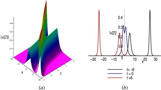
Figure 8. The evolution of the two-soliton solution ∣u[2]∣ given by ( |
5.2. Two-soliton solutions from nonzero seed solution
Choosing the seed solutions u = s, v = r, and solving the linear spectral equation yields
$\begin{eqnarray}\begin{array}{rcl}{\phi }_{4j-3} & = & {d}_{4j-1}{{\rm{e}}}^{{\tau }_{j}x+{m}_{j}t}+{d}_{4j}{{\rm{e}}}^{-{\tau }_{j}x-{m}_{j}t},\\ {\phi }_{4j-2} & = & \left({{as}}^{* }+{b}^{* }s\right){d}_{4j-3}{{\rm{e}}}^{-{\rm{i}}{\lambda }_{j}(x-4{\lambda }_{j}^{2}t)}\\ & & +\displaystyle \frac{{s}^{* }}{{\rm{i}}{\lambda }_{j}+{\tau }_{j}}{d}_{4j-1}{{\rm{e}}}^{{\tau }_{j}x+{m}_{j}t}+\displaystyle \frac{{s}^{* }}{{\rm{i}}{\lambda }_{j}-{\tau }_{j}}{d}_{4j}{{\rm{e}}}^{-{\tau }_{j}x-{m}_{j}t},\\ {\phi }_{4j-1} & = & \left[-\left({as}+{{bs}}^{* }\right){d}_{4j-3}+{{rd}}_{4j-2}\right]{{\rm{e}}}^{-{\rm{i}}{\lambda }_{j}(x-4{\lambda }_{j}^{2}t)}\\ & & +\displaystyle \frac{s}{{\rm{i}}{\lambda }_{j}+{\tau }_{j}}{d}_{4j-1}{{\rm{e}}}^{{\tau }_{j}x+{m}_{j}t}\\ & & +\displaystyle \frac{s}{{\rm{i}}{\lambda }_{j}-{\tau }_{j}}{d}_{4j}{{\rm{e}}}^{-{\tau }_{j}x-{m}_{j}t},\\ {\phi }_{4j} & = & \left({{as}}^{* }+{b}^{* }s\right){d}_{4j-2}{{\rm{e}}}^{-i{\lambda }_{j}(x-4{\lambda }_{j}^{2}t)}\\ & & +\displaystyle \frac{r}{{\rm{i}}{\lambda }_{j}+{\tau }_{j}}{d}_{4j-1}{{\rm{e}}}^{{\tau }_{j}x+{m}_{j}t}\\ & & +\displaystyle \frac{r}{{\rm{i}}{\lambda }_{j}-{\tau }_{j}}{d}_{4j}{{\rm{e}}}^{-{\tau }_{j}x-{m}_{j}t},\end{array}\end{eqnarray}$
where $\begin{eqnarray}\begin{array}{rcl}{\tau }_{j} & = & \sqrt{2a| s{| }^{2}+2\mathrm{Re}({b}^{* }{s}^{2})-{r}^{2}-{\lambda }_{j}^{2}},\\ {m}_{j} & = & -{\tau }_{j}\left(4a| s{| }^{2}+4\mathrm{Re}({b}^{* }{s}^{2})-2{r}^{2}+4{\lambda }_{j}^{2}\right),\\ j & = & 1,2.\end{array}\end{eqnarray}$
Set ${d}_{3}={d}_{7}=\tfrac{{\rm{i}}}{2}$, d4 = d8 = 0, d1 = d2 = d5 = d6 = 1, s = r = 1. We consider the following two cases of solutions.Case 1: $\mathrm{Re}({\tau }_{1})=0$, $\mathrm{Re}({\tau }_{2})=0$. In this case, we have
$\begin{eqnarray}\begin{array}{rcl}{X}_{11} & = & \displaystyle \frac{{\rm{i}}}{108}\left(27+46{{\rm{e}}}^{{\varpi }_{1}}\right),{X}_{22}=\displaystyle \frac{{\rm{i}}}{54}\left(27+46{{\rm{e}}}^{x+t}\right),\\ {Y}_{11} & = & \displaystyle \frac{{\rm{i}}}{36{\left({\rm{i}}\sqrt{3}-3\right)}^{2}}\left[68\left({\rm{i}}\sqrt{3}-1\right){{\rm{e}}}^{{\varpi }_{1}}\right.\\ & & \left.+27\left({\rm{i}}\sqrt{3}-3\right){{\rm{e}}}^{2{\rm{i}}{\varpi }_{2}}\right],\\ {Y}_{22} & = & \displaystyle \frac{{\rm{i}}}{18{\left({\rm{i}}\sqrt{39}-3\right)}^{2}}\left[27\left({\rm{i}}\sqrt{39}-3\right){{\rm{e}}}^{2{\varpi }_{3}}\right.\\ & & \left.+68\left({\rm{i}}\sqrt{39}+5\right){{\rm{e}}}^{x+t}\right],\\ {X}_{21} & = & -\displaystyle \frac{{\rm{i}}}{54\left({\rm{i}}\sqrt{3}-3\right)({\rm{i}}\sqrt{39}+3)}\left[27\left({\rm{i}}\sqrt{39}-{\rm{i}}\sqrt{3}\right.\right.\\ & & \left.+\sqrt{13}+11\right){{\rm{e}}}^{-{\rm{i}}{\varpi }_{3}+{\rm{i}}{\varpi }_{2}}\\ & & \left.+92({\rm{i}}\sqrt{39}-{\rm{i}}\sqrt{3}+\sqrt{13}+3){{\rm{e}}}^{{\varpi }_{4}}\right],\\ {Y}_{21} & = & \displaystyle \frac{{\rm{i}}}{54\left({\rm{i}}\sqrt{3}-3\right)\left({\rm{i}}\sqrt{39}-3\right)}\left[27\left({\rm{i}}\sqrt{39}\right.\right.\\ & & \left.+{\rm{i}}\sqrt{3}+\sqrt{13}-11\right){{\rm{e}}}^{{\rm{i}}{\varpi }_{2}+{\rm{i}}{\varpi }_{3}}\\ & & \left.+68\left({\rm{i}}\sqrt{39}+{\rm{i}}\sqrt{3}+\sqrt{13}-3\right){{\rm{e}}}^{{\varpi }_{4}}\right],\end{array}\end{eqnarray}$
where ϖ1 = 2(x + 4t), ${\varpi }_{2}=\tfrac{\sqrt{3}}{9}(3x+20t)$, ${\varpi }_{3}=\tfrac{\sqrt{39}}{18}(3x+11t)$, ${\varpi }_{4}=\tfrac{3}{2}(x+3t)$. The solution describes the interaction of two breather solutions (see figure 9).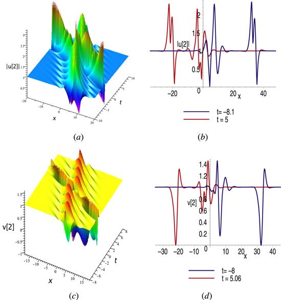
Figure 9. The evolution of two breather solutions with the parameters: λ1 = i, ${\lambda }_{2}=\tfrac{{\rm{i}}}{2}$, $a=-\tfrac{1}{2}$, $b=\tfrac{1}{3}$. (a)–(b) show the ∣u[2]∣. (c)–(d) show the v[2]. |
Case 2: If ${\tau }_{2}\in {\bf{R}},\mathrm{Re}({\tau }_{1})=0$, we have
$\begin{eqnarray*}\begin{array}{rcl}{X}_{11} & = & \displaystyle \frac{{\rm{i}}}{8000}\left(5681{{\rm{e}}}^{{\varpi }_{1}}+2000\right),\\ {Y}_{11} & = & \displaystyle \frac{{\rm{i}}}{800{\left(3{\rm{i}}\sqrt{10}-10\right)}^{2}}\left[2261(6{\rm{i}}\sqrt{10}-1){{\rm{e}}}^{{\varpi }_{1}}\right.\\ & & \left.+2000(3{\rm{i}}\sqrt{10}-1){{\rm{e}}}^{2{\rm{i}}{\varpi }_{5}}\right],\\ {X}_{22} & = & -\displaystyle \frac{{\rm{i}}}{1200{\left(\sqrt{35}-15\right)}^{2}}\left[5681\left(3\sqrt{35}-26\right){{\rm{e}}}^{{\varpi }_{8}}\right.\end{array}\end{eqnarray*}$
$\begin{eqnarray}\begin{array}{rcl} & & \left.+3000\left(\sqrt{35}-15\right){{\rm{e}}}^{2{\varpi }_{6}}\right],\\ {Y}_{22} & = & \displaystyle \frac{{\rm{i}}}{1200{\left(\sqrt{35}-15\right)}^{2}}\left[2261\left(3\sqrt{35}-26\right){{\rm{e}}}^{{\varpi }_{8}}\right.\\ & & \left.+3000\left(\sqrt{35}-15\right){{\rm{e}}}^{2{\varpi }_{6}}\right],\\ {X}_{21} & = & -\displaystyle \frac{{\rm{i}}}{2000\left(3{\rm{i}}\sqrt{10}-10\right)\left(\sqrt{35}-15\right)}\\ & & \left[1000\left(9{\rm{i}}\sqrt{10}-3{\rm{i}}\sqrt{14}+2\sqrt{35}-68\right){{\rm{e}}}^{{\rm{i}}{\varpi }_{5}+{\varpi }_{6}}\right.\\ & & \left.+5681\left(9{\rm{i}}\sqrt{10}-3{\rm{i}}\sqrt{14}+2\sqrt{35}-30\right){{\rm{e}}}^{{\varpi }_{7}}\right],\\ {Y}_{21} & = & \displaystyle \frac{{\rm{i}}}{2000\left(3{\rm{i}}\sqrt{10}-10\right)\left(\sqrt{35}-15\right)}\\ & & \left[1000\left(9{\rm{i}}\sqrt{10}-3{\rm{i}}\sqrt{14}+2\sqrt{35}-68\right){{\rm{e}}}^{{\rm{i}}{\varpi }_{5}+{\varpi }_{6}}\right.\\ & & \left.+2261\left(9{\rm{i}}\sqrt{10}-3{\rm{i}}\sqrt{14}+2\sqrt{35}-30\right){{\rm{e}}}^{{\varpi }_{7}}\right]\end{array}\end{eqnarray}$
where ${\varpi }_{5}=\tfrac{\sqrt{10}}{50}(15x+117t)$, ${\varpi }_{6}=\tfrac{\sqrt{35}}{50}(5x+64t)$, ${\varpi }_{7}=\tfrac{5}{2}(x+7t)$ and ϖ8 = 3x + 27t. In this case, ∣u[2]∣ is a solution describing the interaction of a breather and a soliton solution, and v[2] is a solution describing the interaction of a breather and a kink. Figure 10 gives their evolution process.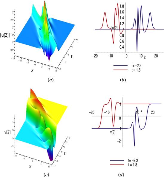
Figure 10. The evolution of solutions ∣u[2]∣ and v[2] with the parameters: λ1 = i, ${\lambda }_{2}=\tfrac{3}{2}{\rm{i}}$, $a=-\tfrac{1}{2}$, $b=\tfrac{1}{20}$. (a)–(b) show the ∣u[2]∣ describing the interaction of a breather and a soliton. (c)–(d) show v[2] describing the interaction of a breather and a kink. |
6. Conclusion
In this paper, we have introduced and studied a two-component gSS equation. A Darboux transformation of the two-component gSS equation has been constructed from its Lax pair. By applying the Darboux transformation, we have obtained its various solutions, including a breather solution, kink solution, anti-soliton solution and periodic-like solution. We should stress that there exists a difference in the soliton solutions between the two-component Sasa-Satsuma equation (5 ) and our two-component gSS equation (6 ), e.g. an anti-soliton solution does not appear for equation (5 ).