Welcome to visit Communications in Theoretical Physics,
Mathematical Physics

Reverse-time type nonlocal Sasa–Satsuma equation and its soliton solutions

  • Xue-Wei Yan ,
  • Yong Chen ,
Expand
  • School of Mathematics, Harbin Institute of Technology, Harbin, 150001, China

Author to whom all correspondence should be addressed.

Received date: 2022-09-06

  Revised date: 2022-11-25

  Accepted date: 2023-02-09

  Online published: 2023-06-26

Copyright

© 2023 Institute of Theoretical Physics CAS, Chinese Physical Society and IOP Publishing

Abstract

In this work, we study the Riemann–Hilbert problem and the soliton solutions for a nonlocal Sasa–Satsuma equation with reverse-time type, which is deduced from a reduction of the coupled Sasa–Satsuma system. Since the coupled Sasa–Satsuma system can describe the dynamic behaviors of two ultrashort pulse envelopes in birefringent fiber, our equation presented here has great physical applications. The classification of soliton solutions is studied in this nonlocal model by considering an inverse scattering transform to the Riemann–Hilbert problem. Simultaneously, we find that the symmetry relations of discrete data in the special nonlocal model are very complicated. Especially, the eigenvectors in the scattering data are determined by the number and location of eigenvalues. Furthermore, multi-soliton solutions are not a simple nonlinear superposition of multiple single-solitons. They exhibit some novel dynamics of solitons, including meandering and sudden position shifts. Also, they have the bound state of multi-soliton entanglement and its interaction with solitons.

Cite this article

Xue-Wei Yan , Yong Chen . Reverse-time type nonlocal Sasa–Satsuma equation and its soliton solutions[J]. Communications in Theoretical Physics, 2023 , 75(7) : 075005 . DOI: 10.1088/1572-9494/acba81

1. Introduction

The nonlinear Schrödinger (NLS) equation plays a key role in mathematical physics, especially in describing soliton propagation in optical fibers. However, the NLS equation only includes the self-phase modulation (SPM) effect and group velocity dispersion (GVD) [1, 2]. Apart from these two terms, there are intensive and short light pulses with widths less than 100 femtoseconds in nonlinear optics, which are also considered in linear and nonlinear effects, such as third-order dispersion (TOD), self-steepening (SS), and stimulated Raman scattering (SRS) [37]. To describe the dynamics of ultrashort pulses, a higher order NLS equation also called Sasa–Satsuma equation was proposed in [811]. When one considers the simultaneous propagation of two ultrashort pulses in birefringent or two-mode fiber, coupled Sasa–Satsuma (CSS) equation included TOD, SS, and SRS was proposed in [1215], and has the form of
$\begin{eqnarray}\begin{array}{l}{\rm{i}}{q}_{1\tau }+\displaystyle \frac{1}{2}{q}_{1\xi \xi }+(| {q}_{1}{| }^{2}+| {q}_{2}{| }^{2}){q}_{1}\\ \,+{\rm{i}}\left[{q}_{1\xi \xi \xi }+6(| {q}_{1}{| }^{2}+| {q}_{2}{| }^{2}){q}_{1\xi }\right.\\ \left.+3{q}_{1}{\left(| {q}_{1}{| }^{2}+| {q}_{2}{| }^{2}\right)}_{\xi }\right]=0,\\ {\rm{i}}{q}_{2\tau }+\displaystyle \frac{1}{2}{q}_{2\xi \xi }+(| {q}_{1}{| }^{2}+| {q}_{2}{| }^{2}){q}_{2}\\ \,+{\rm{i}}\left[{q}_{2\xi \xi \xi }+6(| {q}_{1}{| }^{2}+| {q}_{2}{| }^{2}){q}_{2\xi }\right.\\ \left.+3{q}_{2}{\left(| {q}_{1}{| }^{2}+| {q}_{2}{| }^{2}\right)}_{\xi }\right]=0,\end{array}\end{eqnarray}$
which converts to another form [15]
$\begin{eqnarray}\begin{array}{l}{u}_{t}+{u}_{{xxx}}+6(| u{| }^{2}+| v{| }^{2}){u}_{x}+3u{\left(| u{| }^{2}+| v{| }^{2}\right)}_{x}=0,\\ {v}_{t}+{v}_{{xxx}}+6(| u{| }^{2}+| v{| }^{2}){v}_{x}+3v{\left(| u{| }^{2}+| v{| }^{2}\right)}_{x}=0,\end{array}\end{eqnarray}$
under the gauge, Galilean and scale transformations
$\begin{eqnarray}\begin{array}{l}u(x,t)={q}_{1}(\xi ,\tau ){{\rm{e}}}^{-\tfrac{{\rm{i}}}{6}(\xi -\frac{\tau }{18})},\\ v(x,t)={q}_{2}(\xi ,\tau ){{\rm{e}}}^{-\tfrac{{\rm{i}}}{6}(\xi -\frac{\tau }{18})},\\ x=\xi -\frac{\tau }{12},t=\tau .\end{array}\end{eqnarray}$
The Riemann–Hilbert method is the modern version of the inverse scattering transform. Recently, a lot of interesting and meaningful results have been obtained by applying the Riemann–Hilbert method. For instance, Wang et al studied the general coupled NLS equation and reported the collision dynamics of multi-soliton, recursion operator and conservation laws [16]. Shepelsky studied the Dullin–Gottwald–Holm equation with the Cauchy problem, using Riemann–Hilbert approach. Moreover, smooth and non-smooth cuspon solutions have been researched in [17]. Recently, Ma used the inverse scattering transform to study several types of reverse-spacetime nonlinear integrable equations and obtained various interesting results [1820]. Besides, other important work has been reported in [2126]. In recent years, the method has also been developed to study the asymptotic behaviors of solutions and initial boundary value problems for some integrable equations and has obtained some important results [2738].
In this work, we focus on a physically meaningful nonlocal Sasa–Satsuma equation of reverse time type [39, 40]
$\begin{eqnarray}\begin{array}{l}{u}_{t}+{u}_{{xxx}}+6(| u{| }^{2}+| u(x,-t){| }^{2}){u}_{x}\\ \,+3u{\left(| u{| }^{2}+| u(x,-t){| }^{2}\right)}_{x}=0,\end{array}\end{eqnarray}$
under the constraint
$\begin{eqnarray}v(x,t)={u}^{* }(x,-t)\end{eqnarray}$
in equation (2), where * denotes complex conjugation. The nonlinear induced potential (∣u2 + ∣u(x, −t)∣2) is real and symmetric in t. Equation (4) is derived from a special reduction of another form of the CSS equation, i.e. (2). equations (2) and (4) are two equivalent coupled systems, under constraint (5). By considering the derivation of this nonlocal equation, we can obtain the clear physical interpretation of its solutions. That is to say, equation (4) describes the solutions of the CSS equation, if considering the initial value conditions v(x, 0) = u*(x, 0). Based on this, u(x, t) is determined by equation (4), and v(x, t) is given by v(x, t) = u*(x, −t). For the CSS equation, Tian et al used Darboux transformation to study Dark-bright solitons and semirational rogue wave solutions [41]. Based on the nonlinear steepest descent approach, the long-time asymptotic behavior of solutions has been reported in [40]. Even though the CSS equation has been studied and generated much important work [4244], to the best of our knowledge, its solutions with special initial solutions v(x, 0) = u*(x, 0) have not received much attention.
There is another form of the reverse space-time nonlocal SS equation proposed in [45]. Its periodic solutions, and some localized solutions, such as dark soliton solutions, W-shaped soliton solutions, M-shaped soliton solutions and breather soliton solutions have been investigated by using the binary Darboux transformation method. Various solutions u(x, t) are determined by the nonlocal SS equation, the results of which, provide an important channel for the study of these solutions in the framework of this nonlocal equation. Due to the integrability of the nonlocal SS equation, it is natural to think of seeking its soliton solutions, which also correspond to the solutions of the CSS equation. Thus, we study the multi-soliton solutions of the nonlocal SS equation in the framework of the Riemann–Hilbert problem by using the inverse scattering transform. Our work is developing the Riemann–Hilbert approach to derive the multi-soliton solutions of the nonlocal SS equation, which has not been considered by others. Our goal in this paper is to explain the transmission mechanism of ultrashort pulse solitons in birefringent fiber by constructing the multi-soliton solutions for the nonlocal SS equation.
The paper is organized as follows. In section 2, using a matrix transform derives an equivalent spectral problem, which can be used to obtain a special Riemann–Hilbert problem. In section 3, under reflection-less by using inverse scattering transform to the Riemann–Hilbert problem, some continuous and discrete scattering data can be obtained, and as a result, the general solutions of the Riemann–Hilbert problem can also be obtained. In section 4, the multi-soliton solutions for the nonlocal SS equation can be derived. Finally, some conclusions are presented.

2. Riemann–Hilbert problem

In this section, we consider the direct and inverse scattering problems of equation (4). Equation (4) admits the Lax spectral problem
$\begin{eqnarray}{{\boldsymbol{\psi }}}_{x}=({\rm{i}}\lambda {\boldsymbol{\sigma }}+{\boldsymbol{U}}){\boldsymbol{\psi }},\,\,{{\boldsymbol{\psi }}}_{t}=\left(4{\rm{i}}{\lambda }^{3}{\boldsymbol{\sigma }}+{\boldsymbol{V}}\right){\boldsymbol{\psi }},\end{eqnarray}$
and
$\begin{eqnarray}\begin{array}{rcl}{\boldsymbol{\sigma }} & = & \left(\begin{array}{cc}{{\boldsymbol{I}}}_{4\times 4} & 0\\ 0 & -1\end{array}\right),{\boldsymbol{U}}=\left(\begin{array}{cc}{{\bf{0}}}_{4\times 4} & {\boldsymbol{u}}\\ -{{\boldsymbol{u}}}^{\dagger } & 0\end{array}\right),\\ {\boldsymbol{u}} & = & {\left(u,{u}^{* },{u}^{* }(x,-t),u(x,-t)\right)}^{{\rm{T}}},\\ {\boldsymbol{V}} & = & 4{\lambda }^{2}{\boldsymbol{U}}-2{\rm{i}}\lambda {\boldsymbol{\sigma }}({{\boldsymbol{U}}}_{x}-{{\boldsymbol{U}}}^{2})+{{\boldsymbol{U}}}_{x}{\boldsymbol{U}}\\ & & -{\boldsymbol{U}}{U}_{x}-{{\boldsymbol{U}}}_{{xx}}+2{{\boldsymbol{U}}}^{3},\end{array}\end{eqnarray}$
where † denotes Hermitian conjugation, and T is transpose. Using a transformation
$\begin{eqnarray}{\boldsymbol{\psi }}={\boldsymbol{J}}(x,t){{\rm{e}}}^{{\rm{i}}\left(\lambda x+4{\lambda }^{3}t\right){\boldsymbol{\sigma }}},\end{eqnarray}$
we derive the equivalent matrix spectral problem
$\begin{eqnarray}{{\boldsymbol{J}}}_{x}={\rm{i}}\lambda [{\boldsymbol{\sigma }},{\boldsymbol{J}}]+{\boldsymbol{U}}{\boldsymbol{J}},\end{eqnarray}$
$\begin{eqnarray}{{\boldsymbol{J}}}_{t}=4{\rm{i}}{\lambda }^{3}[{\boldsymbol{\sigma }},{\boldsymbol{J}}]+{\boldsymbol{V}}{\boldsymbol{J}}.\end{eqnarray}$
In order to obtain direct scattering problem, let J± be the Jost solutions for (9) and satisfy the asymptotic conditions
$\begin{eqnarray}{{\boldsymbol{J}}}_{\pm }\to {{\boldsymbol{I}}}_{5\times 5},\,x\to \pm \infty .\end{eqnarray}$
Solving the space evolution (9) we obtain the Volterra integral equations
$\begin{eqnarray}\begin{array}{rcl}{{\boldsymbol{J}}}_{\pm }(x,\lambda ) & = & {{\boldsymbol{I}}}_{5\times 5}\\ & & +{\int }_{\pm \infty }^{x}{{\rm{e}}}^{{\rm{i}}\lambda \tilde{{\boldsymbol{\sigma }}}(x-y)}({\boldsymbol{U}}{{\boldsymbol{J}}}_{\pm })(x,\lambda ,y){\rm{d}}y.\end{array}\end{eqnarray}$
If the right sides of the Volterra integral equations (12) are convergent, then J± exist analytical continuations off the real axis $\lambda \in {\mathbb{R}}$. In addition, J± have a relation that
$\begin{eqnarray}{{\boldsymbol{J}}}_{-}={{\boldsymbol{J}}}_{+}{{\rm{e}}}^{{\rm{i}}\lambda \tilde{{\boldsymbol{\sigma }}}x}{\boldsymbol{S}}(\lambda ),{\boldsymbol{S}}(\lambda )={\left({s}_{{ij}}\right)}_{5\times 5},\,\lambda \in {\mathbb{R}},\end{eqnarray}$
where ${{\rm{e}}}^{\tilde{{\boldsymbol{\sigma }}}}{\boldsymbol{S}}={{\rm{e}}}^{{\boldsymbol{\sigma }}}{\boldsymbol{S}}{{\rm{e}}}^{-{\boldsymbol{\sigma }}}$. Equation (13) indicates $\det ({\boldsymbol{S}}(\lambda ))=1$.
Suppose that J± have the block forms
$\begin{eqnarray}{{\boldsymbol{J}}}_{\pm }=\left({{\boldsymbol{J}}}_{\pm }^{(1)},{{\boldsymbol{J}}}_{\pm }^{(2)},{{\boldsymbol{J}}}_{\pm }^{(3)},{{\boldsymbol{J}}}_{\pm }^{(4)},{{\boldsymbol{J}}}_{\pm }^{(5)}\right),\end{eqnarray}$
where ${{\boldsymbol{J}}}_{\pm }^{(j)},(1\leqslant j\leqslant 5)$ are jth columns of J±. Then the matrix solution
$\begin{eqnarray}{{\boldsymbol{\Psi }}}_{+}={{\boldsymbol{J}}}_{+}{{\boldsymbol{\sigma }}}^{(1)}+{{\boldsymbol{J}}}_{-}{{\boldsymbol{\sigma }}}^{(2)}\end{eqnarray}$
is analytic in upper half-plane ${{\mathbb{C}}}_{+}$ and continuous in closed upper half-plane ${\tilde{{\mathbb{C}}}}_{+}$, where Σ(1) = diag(I4×4, 0), Σ(2) = diag(04×4, 1). The matrix solution
$\begin{eqnarray}{\tilde{{\rm{\Psi }}}}_{+}={{\boldsymbol{J}}}_{-}{{\boldsymbol{\sigma }}}^{(1)}+{{\boldsymbol{J}}}_{+}{{\boldsymbol{\sigma }}}^{(2)}\end{eqnarray}$
is analytic in lower half-plane ${{\mathbb{C}}}_{-}$ and continuous in closed lower half-plane ${\tilde{{\mathbb{C}}}}_{-}$.
Moreover, the Volterra integral equations indicate that
$\begin{eqnarray}\begin{array}{l}{{\rm{\Psi }}}_{+}\to {{\boldsymbol{I}}}_{5\times 5},\,\lambda \in {{\mathbb{C}}}_{+}\to \infty ,\\ {\tilde{{\rm{\Psi }}}}_{+}\to {{\boldsymbol{I}}}_{5\times 5},\,\lambda \in {{\mathbb{C}}}_{-}\to \infty .\end{array}\end{eqnarray}$
Because of the traceless U, using the Volterra integral equations, it follows
$\begin{eqnarray}\det ({{\boldsymbol{J}}}_{\pm })=1,\lambda \in {\mathbb{R}}.\end{eqnarray}$
Next, we consider the analytic counterpart of ψ+ in ${{\mathbb{C}}}_{+}$ from the adjoint spectral problem
$\begin{eqnarray}{{\boldsymbol{K}}}_{x}={\rm{i}}\lambda [{\boldsymbol{\sigma }},{\boldsymbol{K}}]-{\boldsymbol{KU}}.\end{eqnarray}$
Let ${\widetilde{{\boldsymbol{J}}}}_{\pm }={{\boldsymbol{J}}}_{\pm }^{-1}$ solve the adjoint spectral problem (19). Similarly, suppose that ${\widetilde{{\boldsymbol{J}}}}_{\pm }$ are the block matrices
$\begin{eqnarray}{\widetilde{{\boldsymbol{J}}}}_{\pm }={\left({\widetilde{{\boldsymbol{J}}}}_{\pm }^{(1)},{\widetilde{{\boldsymbol{J}}}}_{\pm }^{(2)},{\widetilde{{\boldsymbol{J}}}}_{\pm }^{(3)},{\widetilde{{\boldsymbol{J}}}}_{\pm }^{(4)},{\widetilde{{\boldsymbol{J}}}}_{\pm }^{(5)}\right)}^{{\rm{T}}},\end{eqnarray}$
where ${\widetilde{{\boldsymbol{J}}}}_{\pm }^{(k)}$ are the kth rows of ${\widetilde{{\boldsymbol{J}}}}_{\pm },(1\leqslant k\leqslant 2)$. By using inverse transform to the both sides of (13), one yields
$\begin{eqnarray}{{\boldsymbol{J}}}_{-}^{-1}={{\boldsymbol{S}}}^{-1}(\lambda ){{\rm{e}}}^{-{\rm{i}}\lambda \tilde{\sigma }x}{{\boldsymbol{J}}}_{+}^{-1}\end{eqnarray}$
with
$\begin{eqnarray}{{\boldsymbol{S}}}^{-1}(\lambda )={\left({\hat{s}}_{{ij}}\right)}_{5\times 5}.\end{eqnarray}$
We also find that the adjoint matrix solution
$\begin{eqnarray}{{\boldsymbol{\Psi }}}_{-}={{\boldsymbol{\sigma }}}^{(1)}{{\boldsymbol{J}}}_{+}^{-1}+{{\boldsymbol{\sigma }}}^{(2)}{{\boldsymbol{J}}}_{-}^{-1}\end{eqnarray}$
is analytic in ${{\mathbb{C}}}_{-}$. The matrix solution
$\begin{eqnarray}{\tilde{{\boldsymbol{\Psi }}}}_{-}={{\boldsymbol{\sigma }}}^{(1)}{{\boldsymbol{J}}}_{-}^{-1}+{{\boldsymbol{\sigma }}}^{(2)}{{\boldsymbol{J}}}_{+}^{-1}\end{eqnarray}$
is analytic in ${{\mathbb{C}}}_{+}$. Similar to the asymptotic conditions (17), we also have
$\begin{eqnarray}\begin{array}{l}{{\boldsymbol{\Psi }}}_{-}\to {{\boldsymbol{I}}}_{5\times 5},\,\lambda \in {{\mathbb{C}}}_{-}\to \infty ,\\ {\tilde{{\boldsymbol{\Psi }}}}_{-}\to {{\boldsymbol{I}}}_{5\times 5},\,\lambda \in {{\mathbb{C}}}_{+}\to \infty .\end{array}\end{eqnarray}$
Thus, the matrix functions ψ+ and ψ have been derived. They are analytic in ${{\mathbb{C}}}_{+}$ and ${{\mathbb{C}}}_{-}$, and are continuous in ${\tilde{{\mathbb{C}}}}_{+}$ and ${\tilde{{\mathbb{C}}}}_{-}$, respectively.
We further seek that a relation between ψ+ and ψ on real axis satisfies
$\begin{eqnarray}{\boldsymbol{G}}(x,\lambda )={{\boldsymbol{\Psi }}}_{-}(x,\lambda ){{\boldsymbol{\Psi }}}_{+}(x,\lambda ),\,\lambda \in {\mathbb{R}},\end{eqnarray}$
where
$\begin{eqnarray}{\boldsymbol{G}}(x,\lambda )={{\rm{e}}}^{{\rm{i}}\lambda \tilde{{\boldsymbol{\sigma }}}x}\left(\begin{array}{ccccc}1 & 0 & 0 & 0 & {s}_{15}\\ 0 & 1 & 0 & 0 & {s}_{25}\\ 0 & 0 & 1 & 0 & {s}_{35}\\ 0 & 0 & 0 & 1 & {s}_{45}\\ {\hat{s}}_{51} & {\hat{s}}_{52} & {\hat{s}}_{53} & {\hat{s}}_{54} & 1\end{array}\right).\end{eqnarray}$
Equation (26) is the matrix Riemann–Hilbert problem for the nonlocal SS equation. According to the asymptotic properties in (17) and (25), we obtain the canonical normalization conditions
$\begin{eqnarray}{{\rm{\Psi }}}_{\pm }(x,\lambda )\to {{\boldsymbol{I}}}_{5\times 5},\,\lambda \in {{\mathbb{C}}}_{\pm }\to \infty \end{eqnarray}$
for the Riemann–Hilbert problem (26).
To derive a direct scattering problem, we use the t-derivative of (13) and the vanishing conditions of the potential u, when t → ∞ . It is not hard to get
$\begin{eqnarray}{{\boldsymbol{S}}}_{t}=-2{\rm{i}}{\lambda }^{2}\left[{\boldsymbol{\sigma }},{\boldsymbol{S}}\right],{{\boldsymbol{S}}}_{t}^{-1}=-2{\rm{i}}{\lambda }^{2}\left[{\boldsymbol{\sigma }},{{\boldsymbol{S}}}^{-1}\right],\end{eqnarray}$
from which we derive the time-dependent scattering datum
$\begin{eqnarray}\begin{array}{l}{s}_{15}(\lambda ,t)={s}_{15}(\lambda ,0){{\rm{e}}}^{-4{\rm{i}}{\lambda }^{2}t},\\ {s}_{25}(\lambda ,t)={s}_{25}(\lambda ,0){{\rm{e}}}^{-4{\rm{i}}{\lambda }^{2}t},\\ {s}_{35}(\lambda ,t)={s}_{35}(\lambda ,0){{\rm{e}}}^{-4{\rm{i}}{\lambda }^{2}t},\\ {s}_{45}(\lambda ,t)={s}_{45}(\lambda ,0){{\rm{e}}}^{-4{\rm{i}}{\lambda }^{2}t},\\ {\hat{s}}_{15}(\lambda ,t)={\hat{s}}_{15}(\lambda ,0){{\rm{e}}}^{4{\rm{i}}{\lambda }^{2}t},\\ {\hat{s}}_{25}(\lambda ,t)={\hat{s}}_{25}(\lambda ,0){{\rm{e}}}^{4{\rm{i}}{\lambda }^{2}t},\\ {\hat{s}}_{35}(\lambda ,t)={\hat{s}}_{35}(\lambda ,0){{\rm{e}}}^{4{\rm{i}}{\lambda }^{2}t},\\ {\hat{s}}_{45}(\lambda ,t)={\hat{s}}_{45}(\lambda ,0){{\rm{e}}}^{4{\rm{i}}{\lambda }^{2}t}.\end{array}\end{eqnarray}$
Besides, other scattering datum are independent of t.

3. Inverse scattering transform

In what follows, according to the definitions of $\det ({{\boldsymbol{\Psi }}}_{+})$ and $\det ({{\boldsymbol{\Psi }}}_{-})$, one yields
$\begin{eqnarray}\begin{array}{l}\det ({{\boldsymbol{\Psi }}}_{+})={s}_{55},\,\lambda \in {{\mathbb{C}}}_{+},\\ \det ({{\boldsymbol{\Psi }}}_{-})={\hat{s}}_{55},\,\lambda \in {{\mathbb{C}}}_{-}.\end{array}\end{eqnarray}$
This shows that $\det ({{\boldsymbol{\Psi }}}_{+})$ and $\det ({{\boldsymbol{\Psi }}}_{-})$ have the same zero points as ${s}_{55},{\hat{s}}_{55}$, respectively. Equation (21) satisfies
$\begin{eqnarray}{{\boldsymbol{J}}}_{\pm }^{\dagger }({\lambda }^{* })={{\boldsymbol{J}}}_{\pm }^{-1}(\lambda ).\end{eqnarray}$
According to equation (13), we can obtain
$\begin{eqnarray}{{\boldsymbol{S}}}^{\dagger }({\lambda }^{* })={{\boldsymbol{S}}}^{-1}(\lambda ),\end{eqnarray}$
where the entries of S, S−1 satisfy
$\begin{eqnarray}{\hat{s}}_{51}(\lambda )={s}_{15}^{* }(\lambda ),{\hat{s}}_{52}(\lambda )={s}_{25}^{* }(\lambda ),\end{eqnarray}$
$\begin{eqnarray}{\hat{s}}_{53}(\lambda )={s}_{35}^{* }(\lambda ),{\hat{s}}_{54}(\lambda )={s}_{45}^{* }(\lambda ),\end{eqnarray}$
$\begin{eqnarray}{\hat{s}}_{55}^{* }({\lambda }^{* })={s}_{55}(\lambda ),\lambda \in {{\mathbb{C}}}_{+}.\end{eqnarray}$
Moreover, we find U satisfies the two symmetry relations
$\begin{eqnarray}{{\boldsymbol{U}}}^{* }(x,-t)={\boldsymbol{\Delta }}{\boldsymbol{U}}(x,t){\boldsymbol{\Delta }},{\boldsymbol{U}}{\left(x,t\right)}^{\dagger }=-{\boldsymbol{U}}(x,t)\end{eqnarray}$
with
$\begin{eqnarray}{\boldsymbol{\Delta }}=\left(\begin{array}{ccccc}0 & 1 & 0 & 0 & 0\\ 1 & 0 & 0 & 0 & 0\\ 0 & 0 & 0 & 1 & 0\\ 0 & 0 & 1 & 0 & 0\\ 0 & 0 & 0 & 0 & 1\end{array}\right),\end{eqnarray}$
which arrives at
$\begin{eqnarray}{\boldsymbol{\Delta }}{{\boldsymbol{J}}}_{\pm }(x,-t,-{\lambda }^{* }){\boldsymbol{\Delta }}={{\boldsymbol{J}}}_{\pm }^{* }(x,t,\lambda ),\end{eqnarray}$
$\begin{eqnarray}{\boldsymbol{\Delta }}{{\boldsymbol{J}}}_{\pm }^{\dagger }(x,t,{\lambda }^{* }){\boldsymbol{\Delta }}={{\boldsymbol{J}}}_{\pm }^{-1}(x,t,\lambda ).\end{eqnarray}$
Actually, S satisfies ΔS( − λ*)Δ = S(λ), which follows that
$\begin{eqnarray}{\boldsymbol{\Delta }}{{\boldsymbol{\Psi }}}_{+}(x,-t,-{\lambda }^{* }){\boldsymbol{\Delta }}={{\boldsymbol{\Psi }}}_{+}^{* }(x,t,\lambda ),\lambda \in {{\mathbb{C}}}_{+},\end{eqnarray}$
$\begin{eqnarray}{{\boldsymbol{\Psi }}}_{+}^{\dagger }(x,t,{\lambda }^{* })={{\boldsymbol{\Psi }}}_{-}(x,t,\lambda ),\lambda \in {{\mathbb{C}}}_{-}.\end{eqnarray}$

$\det ({{\boldsymbol{\Psi }}}_{\pm })$ have three types of zero structures as follows.

I

(I)$\det ({{\boldsymbol{\Psi }}}_{+})$ has 2N1 simple zeros ${\lambda }_{j},(1\leqslant j\leqslant 2{N}_{1})$ in ${{\mathbb{C}}}_{+}$, where ${\lambda }_{{N}_{1}+l}=-{\lambda }_{l}^{* },(1\leqslant l\leqslant {N}_{1})$. Then $\det ({{\boldsymbol{\Psi }}}_{-})$ has 2N1 zeros ${\hat{\lambda }}_{j},(1\leqslant j\leqslant 2{N}_{1})$ in ${{\mathbb{C}}}_{-}$, where ${\hat{\lambda }}_{j}={\lambda }_{j}^{* }$.

II

(II)$\det ({{\boldsymbol{\Psi }}}_{+})$ has N2 purely imaginary zeros ${\lambda }_{j},(1\leqslant j\leqslant {N}_{2})$ in ${{\mathbb{C}}}_{+}$. Then $\det ({{\boldsymbol{\Psi }}}_{-})$ has N2 purely imaginary zeros ${\hat{\lambda }}_{j}={\lambda }_{j}^{* },(1\leqslant j\leqslant {N}_{2})$ in ${{\mathbb{C}}}_{-}$.

III

(III)$\det ({{\boldsymbol{\Psi }}}_{+})$ has $2{N}_{1}+{N}_{2}$ simple zeros ${\lambda }_{j},(1\,\leqslant j\,\leqslant 2{N}_{1}+{N}_{2})$ in ${{\mathbb{C}}}_{+}$, where ${\lambda }_{{N}_{1}+l}=-{\lambda }_{l}^{* },(1\,\leqslant l\leqslant {N}_{1})$ and ${\lambda }_{2{N}_{1}+l}\in {\rm{i}}{\mathbb{R}}$. Then $\det ({{\boldsymbol{\Psi }}}_{-})$ has $2{N}_{1}+{N}_{2}$ simple zeros ${\hat{\lambda }}_{j}={\lambda }_{j}^{* },(1\leqslant j\leqslant 2{N}_{1}+{N}_{2})$ in ${{\mathbb{C}}}_{-}$.

Equation (41) implies that λ is a zero of $\det ({{\boldsymbol{\Psi }}}_{+})$, so is $-{\lambda }^{* }$. Equation (42) implies that ${\lambda }^{* }$ is a zero of $\det ({{\boldsymbol{\Psi }}}_{-})$, if λ is a zero of $\det ({{\boldsymbol{\Psi }}}_{+})$. This completes the proof.

In order to obtain the general solution for the Riemann–Hilbert problem (26), we need to derive the continuous scattering datum ${s}_{15},{s}_{25},{s}_{35},{s}_{45},{\hat{s}}_{51},{\hat{s}}_{52},{\hat{s}}_{53},{\hat{s}}_{54}$ and the discrete scattering datum ${\lambda }_{j},{\hat{\lambda }}_{j},{{\boldsymbol{v}}}_{j},{\hat{{\boldsymbol{v}}}}_{j}$, where ${{\boldsymbol{v}}}_{j},{\hat{{\boldsymbol{v}}}}_{j}$ represent the nonzero column and row vectors, and satisfy
$\begin{eqnarray}{{\boldsymbol{\Psi }}}_{+}({\lambda }_{j}){{\boldsymbol{v}}}_{j}=0,\,{\hat{{\boldsymbol{v}}}}_{j}{{\boldsymbol{\Psi }}}_{-}({\hat{\lambda }}_{j})=0,\end{eqnarray}$
respectively.
According to case (I), we know that $\det ({{\boldsymbol{\Psi }}}_{+})$ has 2N1 zeros λj, (1 ≤ j ≤ 2N1) in ${{\mathbb{C}}}_{+}$, where ${\lambda }_{{N}_{1}+l}=-{\lambda }_{l}^{* },(1\leqslant l\leqslant {N}_{1})$. Then the zeros of $\det ({{\boldsymbol{\Psi }}}_{-})$ are conjugated to the zeros of $\det ({{\boldsymbol{\Psi }}}_{+})$. The symmetry (41) gives the relation of $\det ({{\boldsymbol{\Psi }}}_{+})$ at (x, − t, − λ*) and (x, t, λ). The symmetry (42) indicates that $\det ({{\boldsymbol{\Psi }}}_{+})$ at (x, t, λ*) equates to $\det ({{\boldsymbol{\Psi }}}_{-})$ at (x, t, λ). Thus, based on (43) and ${\lambda }_{{N}_{1}+l}=-{\lambda }_{l}^{* }$, we have the symmetries
$\begin{eqnarray}{{\boldsymbol{v}}}_{{N}_{1}+l}(x,t)={\boldsymbol{\Delta }}{{\boldsymbol{v}}}_{l}^{* }(x,-t),\,1\leqslant l\leqslant {N}_{1},\end{eqnarray}$
$\begin{eqnarray}{\hat{{\boldsymbol{v}}}}_{j}(x,t)={{\boldsymbol{v}}}_{j}^{\dagger }(x,t),\,1\leqslant j\leqslant 2{N}_{1}.\end{eqnarray}$
This indicates that one only needs to solve vj, (1 ≤ jN1), such that all vectors vj and ${\hat{{\boldsymbol{v}}}}_{j}$ can be obtained. Thus by taking the x, t-derivatives of the first expression in equation (43) and integrating it, we have
$\begin{eqnarray}{{\boldsymbol{v}}}_{j}=\left\{\begin{array}{ll}{{\rm{e}}}^{{\theta }_{j}{\boldsymbol{\sigma }}}{{\boldsymbol{v}}}_{j,0}, & 1\leqslant j\leqslant {N}_{1},\\ {\boldsymbol{\Delta }}{{\rm{e}}}^{{\theta }_{j-{N}_{1}}^{* }(x,-t)\sigma }{{\boldsymbol{v}}}_{j-{N}_{1},0}^{* }, & {N}_{1}+1\leqslant j\leqslant 2{N}_{1},\end{array}\right.\end{eqnarray}$
and
$\begin{eqnarray}{\hat{{\boldsymbol{v}}}}_{j}=\left\{\begin{array}{ll}{{\boldsymbol{v}}}_{j,0}^{\dagger }{{\rm{e}}}^{{\theta }_{j}^{* }{\boldsymbol{\sigma }}}, & 1\leqslant j\leqslant {N}_{1},\\ {{\boldsymbol{v}}}_{j-{N}_{1},0}^{{\prime} }{{\rm{e}}}^{{\theta }_{j-{N}_{1}}(x,-t){\boldsymbol{\sigma }}}{\boldsymbol{\Delta }}, & {N}_{1}+1\leqslant j\leqslant 2{N}_{1},\end{array}\right.\end{eqnarray}$
where ${\theta }_{j}(x,t)={\rm{i}}{\lambda }_{j}x+4{\rm{i}}{\lambda }_{j}^{3}t,{\lambda }_{j}\in {{\mathbb{C}}}_{+},{\lambda }_{{jR}}\ne 0$, and vj,0 are column vectors independent of x, t.
Next, we introduce the matrices
$\begin{eqnarray}\begin{array}{rcl}{{\boldsymbol{\Phi }}}_{+}(\lambda ) & = & {\boldsymbol{I}}-\displaystyle \sum _{k=1}^{2{N}_{1}}\displaystyle \sum _{j=1}^{2{N}_{1}}\displaystyle \frac{{{\boldsymbol{v}}}_{k}{\hat{{\boldsymbol{v}}}}_{j}{\left({{\boldsymbol{M}}}^{-1}\right)}_{{kj}}}{\lambda -{\hat{\lambda }}_{j}},\lambda \in {{\mathbb{C}}}_{+}\cup {\mathbb{R}},\\ {{\boldsymbol{\Phi }}}_{-}(\lambda ) & = & {\boldsymbol{I}}+\displaystyle \sum _{k=1}^{2{N}_{1}}\displaystyle \sum _{j=1}^{2{N}_{1}}\displaystyle \frac{{{\boldsymbol{v}}}_{k}{\hat{{\boldsymbol{v}}}}_{j}{\left({{\boldsymbol{M}}}^{-1}\right)}_{{kj}}}{\lambda -{\lambda }_{k}},\lambda \in {{\mathbb{C}}}_{-}\cup {\mathbb{R}},\end{array}\end{eqnarray}$
where ${\boldsymbol{M}}={\left({m}_{{kj}}\right)}_{2{N}_{1}\times 2{N}_{1}}$ is an invertible matrix, and
$\begin{eqnarray}{m}_{{kj}}=\displaystyle \frac{{\hat{{\boldsymbol{v}}}}_{k}{{\boldsymbol{v}}}_{j}}{{\lambda }_{j}-{\hat{\lambda }}_{k}},1\leqslant j\leqslant 2{N}_{1}.\end{eqnarray}$
Using Φ±(λ), we regulate the Riemann–Hilbert problem (26) to a regular one. Then, it satisfies
$\begin{eqnarray}\begin{array}{rcl}{{\boldsymbol{\Psi }}}_{+}(\lambda ) & = & {{\boldsymbol{\Omega }}}_{+}(\lambda ){{\boldsymbol{\Phi }}}_{+}(\lambda ),\\ {{\boldsymbol{\Psi }}}_{-}(\lambda ) & = & {{\boldsymbol{\Phi }}}_{-}(\lambda ){{\boldsymbol{\Omega }}}_{-}(\lambda ),\end{array}\end{eqnarray}$
where ω±(λ) satisfy
$\begin{eqnarray}\begin{array}{rcl}{{\boldsymbol{\Omega }}}_{+}^{-1}(\lambda ) & = & {\boldsymbol{I}}+\displaystyle \frac{1}{2\pi {\rm{i}}}{\int }_{-\infty }^{+\infty }\displaystyle \frac{{{\boldsymbol{\Phi }}}_{+}(y)[{\boldsymbol{I}}-{\boldsymbol{G}}(y)]{{\boldsymbol{\Phi }}}_{-}(y){{\boldsymbol{\Omega }}}_{+}^{-1}(y)}{y-\lambda }{\rm{d}}y,\\ {{\boldsymbol{\Omega }}}_{-}(\lambda ) & = & {\boldsymbol{I}}+\displaystyle \frac{1}{2\pi {\rm{i}}}{\int }_{-\infty }^{+\infty }\displaystyle \frac{{{\boldsymbol{\Phi }}}_{+}(y)[{\boldsymbol{I}}-{\boldsymbol{G}}(y)]{{\boldsymbol{\Phi }}}_{-}(y){{\boldsymbol{\Omega }}}_{-}(y)}{y-\lambda }{\rm{d}}y\end{array}\end{eqnarray}$
with
$\begin{eqnarray}\begin{array}{rcl}{\boldsymbol{G}}(y) & = & {{\rm{e}}}^{{\rm{i}}({\lambda }_{j}x+4{\lambda }_{j}^{3}t)\tilde{{\boldsymbol{\sigma }}}}\\ & & \times \left(\begin{array}{ccccc}1 & 0 & 0 & 0 & -{\hat{s}}_{15}(0,y)\\ 0 & 1 & 0 & 0 & -{\hat{s}}_{25}(0,y)\\ 0 & 0 & 1 & 0 & -{\hat{s}}_{35}(0,y)\\ 0 & 0 & 0 & 1 & -{\hat{s}}_{45}(0,y)\\ -{s}_{51}(0,y) & -{s}_{52}(0,y) & -{s}_{53}(0,y) & -{s}_{54}(0,y) & 1\end{array}\right).\end{array}\end{eqnarray}$
If ${s}_{5j},{\hat{s}}_{j5},(1\leqslant j\leqslant 4)$ are nonzero constants, i.e. the Riemann–Hilbert problem (26) contains reflection data, precise solutions can not be obtained, due to the imprecisely solvable integrable equations (51) w.r.t. ω±. Hence, in order to construct explicit soliton solutions, the Riemann–Hilbert problem is needed to be reconsidered under reflection-less. Calculating the Riemann–Hilbert problem (26), one has the following solutions
$\begin{eqnarray}{{\boldsymbol{\Psi }}}_{+}(\lambda )={\boldsymbol{I}}-\displaystyle \sum _{k=1}^{2{N}_{1}}\displaystyle \sum _{j=1}^{2{N}_{1}}\displaystyle \frac{{{\boldsymbol{v}}}_{k}{\hat{{\boldsymbol{v}}}}_{j}{\left({{\boldsymbol{M}}}^{-1}\right)}_{{kj}}}{\lambda -{\hat{\lambda }}_{j}},\end{eqnarray}$
$\begin{eqnarray}{{\boldsymbol{\Psi }}}_{-}(\lambda )={\boldsymbol{I}}+\displaystyle \sum _{k=1}^{2{N}_{1}}\displaystyle \sum _{j=1}^{2{N}_{1}}\displaystyle \frac{{{\boldsymbol{v}}}_{k}{\hat{{\boldsymbol{v}}}}_{j}{\left({{\boldsymbol{M}}}^{-1}\right)}_{{kj}}}{\lambda -{\lambda }_{k}},\end{eqnarray}$
where ${\boldsymbol{M}}={\left({m}_{{kj}}\right)}_{2{N}_{1}\times 2{N}_{1}}$ is an invertible matrix with
$\begin{eqnarray}{m}_{{kj}}=\displaystyle \frac{{\hat{{\boldsymbol{v}}}}_{k}{{\boldsymbol{v}}}_{j}}{{\lambda }_{j}-{\hat{\lambda }}_{k}},1\leqslant j\leqslant 2{N}_{1}.\end{eqnarray}$
For case (II), $\det ({{\boldsymbol{\Psi }}}_{+})$ has N2 zeros ${\lambda }_{j}\in {\rm{i}}{\mathbb{R}},(1\leqslant j\leqslant {N}_{2})$ in ${{\mathbb{C}}}_{+}$. Then the zeros of $\det ({{\boldsymbol{\Psi }}}_{-})$ are conjugated to the zeros of $\det ({{\boldsymbol{\Psi }}}_{+})$. Similar to case (I), the vectors ${{\boldsymbol{v}}}_{j},{\hat{{\boldsymbol{v}}}}_{j},(1\leqslant j\leqslant {N}_{2})$ arrive at
$\begin{eqnarray}\left\{\begin{array}{l}{{\boldsymbol{v}}}_{j}={{\rm{e}}}^{{\theta }_{j}{\boldsymbol{\sigma }}}{{\boldsymbol{v}}}_{j,0},\\ {\hat{{\boldsymbol{v}}}}_{j}={{\boldsymbol{v}}}_{j,0}^{\dagger }{{\rm{e}}}^{{\theta }_{j}^{* }{\boldsymbol{\sigma }}},\end{array}\right.\end{eqnarray}$
where θj(x, t), (1 ≤ jN2) are the same as (46)–(47). Thus, under the case of reflection-less, the general solutions for the Riemann–Hilbert problem (26) are given by
$\begin{eqnarray}{{\boldsymbol{\Psi }}}_{+}(\lambda )={{\boldsymbol{I}}}_{5\times 5}-\displaystyle \sum _{k=1}^{{N}_{2}}\displaystyle \sum _{j=1}^{{N}_{2}}\displaystyle \frac{{{\boldsymbol{v}}}_{k}{\hat{{\boldsymbol{v}}}}_{j}{\left({{\boldsymbol{M}}}^{-1}\right)}_{{kj}}}{\lambda -{\hat{\lambda }}_{j}},\end{eqnarray}$
$\begin{eqnarray}{{\boldsymbol{\Psi }}}_{-}(\lambda )={{\boldsymbol{I}}}_{5\times 5}+\displaystyle \sum _{k=1}^{{N}_{2}}\displaystyle \sum _{j=1}^{{N}_{2}}\displaystyle \frac{{{\boldsymbol{v}}}_{k}{\hat{{\boldsymbol{v}}}}_{j}{\left({{\boldsymbol{M}}}^{-1}\right)}_{{kj}}}{\lambda -{\lambda }_{k}},\end{eqnarray}$
where the elements mkj of M are the same as (55), besides 1 ≤ jN2.
For case (III), as a combination of the first two cases, its discrete scattering datum has the following results
$\begin{eqnarray}{{\boldsymbol{v}}}_{j}=\left\{\begin{array}{ll}{{\rm{e}}}^{{\theta }_{j}{\boldsymbol{\sigma }}}{{\boldsymbol{v}}}_{j,0}, & 1\leqslant j\leqslant {N}_{1},\mathrm{and}\,2{N}_{1}+1\leqslant j\leqslant 2{N}_{1}+{N}_{2},\\ {\boldsymbol{\Delta }}{{\rm{e}}}^{{\theta }_{j-{N}_{1}}^{* }(x,-t){\boldsymbol{\sigma }}}{{\boldsymbol{v}}}_{j-{N}_{1},0}^{* }, & {N}_{1}+1\leqslant j\leqslant 2{N}_{1},\end{array}\right.\end{eqnarray}$
and
$\begin{eqnarray}{\hat{{\boldsymbol{v}}}}_{j}=\left\{\begin{array}{ll}{{\boldsymbol{v}}}_{j,0}^{\dagger }{{\rm{e}}}^{{\theta }_{j}^{* }{\boldsymbol{\sigma }}}, & 1\leqslant j\leqslant {N}_{1},\mathrm{and}\,2{N}_{1}+1\leqslant j\leqslant 2{N}_{1}+{N}_{2},\\ {{\boldsymbol{v}}}_{j-{N}_{1},0}^{\dagger }{{\rm{e}}}^{{\theta }_{j-{N}_{1}}(x,-t){\boldsymbol{\sigma }}}{\boldsymbol{\Delta }}, & {N}_{1}+1\leqslant j\leqslant 2{N}_{1},\end{array}\right.\end{eqnarray}$
where θj(x, t), (1 ≤ j ≤ 2N1 + N2) are the same as (46)–(47). Without loss of generality, the general solutions of the Riemann–Hilbert problem (26) are
$\begin{eqnarray}{{\boldsymbol{\Psi }}}_{+}(\lambda )={{\boldsymbol{I}}}_{5\times 5}-\displaystyle \sum _{k=1}^{2{N}_{1}+{N}_{2}}\displaystyle \sum _{j=1}^{2{N}_{1}+{N}_{2}}\displaystyle \frac{{{\boldsymbol{v}}}_{k}{\hat{{\boldsymbol{v}}}}_{j}{\left({{\boldsymbol{M}}}^{-1}\right)}_{{kj}}}{\lambda -{\hat{\lambda }}_{j}},\end{eqnarray}$
$\begin{eqnarray}{{\boldsymbol{\Psi }}}_{-}(\lambda )={{\boldsymbol{I}}}_{5\times 5}+\displaystyle \sum _{k=1}^{2{N}_{1}+{N}_{2}}\displaystyle \sum _{j=1}^{2{N}_{1}+{N}_{2}}\displaystyle \frac{{{\boldsymbol{v}}}_{k}{\hat{{\boldsymbol{v}}}}_{j}{\left({{\boldsymbol{M}}}^{-1}\right)}_{{kj}}}{\lambda -{\lambda }_{k}},\end{eqnarray}$
where the forms of the elements of M are the same as (55), besides 1 ≤ j ≤ 2N1 + N2.
Now, we consider the asymptotic expansion of ψ+(λ)
$\begin{eqnarray}{{\boldsymbol{\Psi }}}_{+}(\lambda )={{\boldsymbol{I}}}_{5\times 5}+\displaystyle \frac{{{\boldsymbol{\Psi }}}_{+}^{(1)}}{\lambda }+\displaystyle \frac{{{\boldsymbol{\Psi }}}_{+}^{(2)}}{{\lambda }^{2}}+\cdots ,\,\lambda \to \infty ,\end{eqnarray}$
which can be used to reconstruct the potential u. Substituting (63) into (9), we have
$\begin{eqnarray}\begin{array}{rcl}{\boldsymbol{U}} & = & -{\rm{i}}\left[{\boldsymbol{\sigma }},{{\boldsymbol{\Psi }}}_{+}^{(1)}\right]\\ & = & \left(\begin{array}{ccccc}0 & 0 & 0 & 0 & -2{\rm{i}}{{\boldsymbol{\Psi }}}_{+,15}^{(1)}\\ 0 & 0 & 0 & 0 & -2{\rm{i}}{{\boldsymbol{\Psi }}}_{+,25}^{(1)}\\ 0 & 0 & 0 & 0 & -2{\rm{i}}{{\boldsymbol{\Psi }}}_{+,35}^{(1)}\\ 0 & 0 & 0 & 0 & -2{\rm{i}}{{\boldsymbol{\Psi }}}_{+,45}^{(1)}\\ 2{\rm{i}}{{\boldsymbol{\Psi }}}_{+,51}^{(1)} & 2{\rm{i}}{{\boldsymbol{\Psi }}}_{+,52}^{(1)} & 2{\rm{i}}{{\boldsymbol{\Psi }}}_{+,53}^{(1)} & 2{\rm{i}}{{\boldsymbol{\Psi }}}_{+,54}^{(1)} & 0\end{array}\right),\end{array}\end{eqnarray}$
which implies that,
$\begin{eqnarray}u(x,t)=-2{\rm{i}}{{\boldsymbol{\Psi }}}_{+,15}^{(1)},u(x,-t)=-2{\rm{i}}{{\boldsymbol{\Psi }}}_{+,45}^{(1)}.\end{eqnarray}$
According to (53), (57) and (63), ${{\boldsymbol{\Psi }}}_{+}^{(1)}$ respectively corresponds to the following expressions
$\begin{eqnarray}{{\boldsymbol{\Psi }}}_{+}^{(1)}=\left\{\begin{array}{l}-\displaystyle \sum _{k=1}^{2{N}_{1}}\displaystyle \sum _{j=1}^{2{N}_{1}}{{\boldsymbol{v}}}_{k}{\hat{{\boldsymbol{v}}}}_{j}{\left({{\boldsymbol{M}}}^{-1}\right)}_{{kj}},\\ -\displaystyle \sum _{k=1}^{{N}_{2}}\displaystyle \sum _{j=1}^{{N}_{2}}{{\boldsymbol{v}}}_{k}{\hat{{\boldsymbol{v}}}}_{j}{\left({{\boldsymbol{M}}}^{-1}\right)}_{{kj}},\\ -\displaystyle \sum _{k=1}^{2{N}_{1}+{N}_{2}}\displaystyle \sum _{j=1}^{2{N}_{1}+{N}_{2}}{{\boldsymbol{v}}}_{k}{\hat{{\boldsymbol{v}}}}_{j}{\left({{\boldsymbol{M}}}^{-1}\right)}_{{kj}}.\end{array}\right.\end{eqnarray}$

4. Soliton solutions for the Riemann–Hilbert problem

According to the three types of zero structures of $\det ({{\boldsymbol{\Psi }}}_{\pm })$ presented in theorem 3.1, we derive the multi-soliton solutions for the nonlocal SS equation in this section.

Assume that ${\lambda }_{{jR}}\ne 0$, ${\lambda }_{{jI}}\gt 0$, ${{\boldsymbol{v}}}_{j,0}\,={\left({a}_{1j},{a}_{2j},{a}_{3j},{a}_{4j},1\right)}^{{\rm{T}}}$, $(1\leqslant j\leqslant 2{N}_{1})$, where ${\lambda }_{{jR}},{\lambda }_{{jI}}$ denote real and imaginary parts of ${\lambda }_{j}$, respectively. The nonlocal SS equation has the 2N1-soliton solution

$\begin{eqnarray}\begin{array}{rcl}{u}_{2{N}_{1}} & = & 2{\rm{i}}\displaystyle \sum _{k=1}^{{N}_{1}}\displaystyle \sum _{j=1}^{{N}_{1}}{a}_{1k}{{\rm{e}}}^{{\theta }_{k}-{\theta }_{j}^{* }}{\left({{\boldsymbol{M}}}^{-1}\right)}_{{kj}}\\ & & +2{\rm{i}}\displaystyle \sum _{k=1}^{{N}_{1}}\displaystyle \sum _{j={N}_{1}+1}^{2{N}_{1}}{a}_{1k}{{\rm{e}}}^{{\theta }_{k}-{\theta }_{j-{N}_{1}}(x,-t)}{\left({{\boldsymbol{M}}}^{-1}\right)}_{{kj}}\\ & & +2{\rm{i}}\displaystyle \sum _{k={N}_{1}+1}^{2{N}_{1}}\displaystyle \sum _{j=1}^{{N}_{1}}{a}_{2,k-{N}_{1}}^{* }{{\rm{e}}}^{{\theta }_{k-{N}_{1}}^{* }(x,-t)-{\theta }_{j}^{* }}{\left({{\boldsymbol{M}}}^{-1}\right)}_{{kj}}\\ & & +2{\rm{i}}\displaystyle \sum _{k={N}_{1}+1}^{2{N}_{1}}\displaystyle \sum _{j={N}_{1}+1}^{2{N}_{1}}{a}_{2,k-{N}_{1}}^{* }{{\rm{e}}}^{{\theta }_{k-{N}_{1}}^{* }(x,-t)-{\theta }_{j-{N}_{1}}(x,-t)}{\left({{\boldsymbol{M}}}^{-1}\right)}_{{kj}},\end{array}\end{eqnarray}$
where ${\boldsymbol{M}}={\left({m}_{{kj}}\right)}_{2{N}_{1}\times 2{N}_{1}}$ satisfies
$\begin{eqnarray}{m}_{{kj}}=\left\{\begin{array}{l}\displaystyle \frac{{{\rm{e}}}^{-{\theta }_{k}^{* }-{\theta }_{j}}+\displaystyle \sum _{\iota =1}^{4}{a}_{\iota k}^{* }{a}_{\iota j}{{\rm{e}}}^{{\theta }_{k}^{* }+{\theta }_{j}}}{{\lambda }_{j}-{\lambda }_{k}^{* }},1\leqslant k,j\leqslant {N}_{1},\\ \displaystyle \frac{{{\rm{e}}}^{-{\theta }_{k}^{* }-{\theta }_{j-{N}_{1}}^{* }(x,-t)}+{\eta }_{k,j-{N}_{1}}^{* }{{\rm{e}}}^{{\theta }_{k}^{* }+{\theta }_{j-{N}_{1}}^{* }(x,-t)}}{-{\lambda }_{j-{N}_{1}}^{* }-{\lambda }_{k}^{* }},\,1\leqslant k\leqslant {N}_{1},{N}_{1}+1\leqslant j\leqslant 2{N}_{1},\\ \displaystyle \frac{{{\rm{e}}}^{-{\theta }_{k-{N}_{1}}(x,-t)-{\theta }_{j}}+{\eta }_{j,k-{N}_{1}}{{\rm{e}}}^{{\theta }_{k-{N}_{1}}(x,-t)+{\theta }_{j}}}{{\lambda }_{j}+{\lambda }_{k-{N}_{1}}},{N}_{1}+1\leqslant k\leqslant 2{N}_{1},1\leqslant j\leqslant {N}_{1},\\ \displaystyle \frac{{{\rm{e}}}^{-{\theta }_{k-{N}_{1}}(x,-t)-{\theta }_{j-{N}_{1}}^{* }(x,-t)}+\displaystyle \sum _{\iota =1}^{4}{a}_{\iota ,k-{N}_{1}}{a}_{\iota ,j-{N}_{1}}^{* }{e}^{{\theta }_{k-{N}_{1}}(x,-t)+{\theta }_{j-{N}_{1}}^{* }(x,-t)}}{-{\lambda }_{j-{N}_{1}}^{* }+{\lambda }_{k-{N}_{1}}},{N}_{1}+1\leqslant k,j\leqslant 2{N}_{1},\\ {\eta }_{r,s}={a}_{1r}{a}_{2,s}+{a}_{2r}{a}_{1,s}+{a}_{3r}{a}_{4,s}+{a}_{4r}{a}_{3,s}.\end{array}\right.\end{eqnarray}$

Based on equations (46)–(47) and equations (65)–(66), one can easily obtain this solution.

Furthermore, we can write the 2N1-soliton solution as determinant form
$\begin{eqnarray}{u}_{2{N}_{1}}=2{\rm{i}}\displaystyle \frac{\det ({\boldsymbol{H}})}{\det ({\boldsymbol{M}})},\end{eqnarray}$
where H is given by
$\begin{eqnarray}{\boldsymbol{H}}=\left(\begin{array}{cc}0 & {{\boldsymbol{m}}}_{1}\\ {{\boldsymbol{n}}}_{1} & {{\boldsymbol{M}}}_{2{N}_{1}\times 2{N}_{1}}\end{array}\right)\end{eqnarray}$
with
$\begin{eqnarray}\begin{array}{rcl}{{\boldsymbol{n}}}_{1} & = & {\left({{\rm{e}}}^{-{\theta }_{1}^{* }},\ldots ,{{\rm{e}}}^{-{\theta }_{{N}_{1}}^{* }},{{\rm{e}}}^{-{\theta }_{1}(x,-t)},\ldots ,{{\rm{e}}}^{-{\theta }_{{N}_{1}}(x,-t)}\right)}^{{\rm{T}}},\\ {{\boldsymbol{m}}}_{1} & = & ({a}_{11}{{\rm{e}}}^{{\theta }_{1}},\ldots ,{a}_{1{N}_{1}}{{\rm{e}}}^{{\theta }_{{N}_{1}}},{a}_{21}^{* }{{\rm{e}}}^{{\theta }_{1}^{* }(x,-t)},\ldots ,{a}_{2{N}_{1}}^{* }{{\rm{e}}}^{{\theta }_{{N}_{1}}^{* }(x,-t)}).\end{array}\end{eqnarray}$

Assume that ${\lambda }_{{jR}}=0$, ${\lambda }_{{jI}}\gt 0$, ${{\boldsymbol{v}}}_{j,0}={\left({b}_{1j},{b}_{2j},{b}_{3j},{b}_{4j},1\right)}^{{\rm{T}}}$, $(1\leqslant j\leqslant {N}_{2})$. The N2-soliton solution is

$\begin{eqnarray}{u}_{{N}_{2}}=2{\rm{i}}\displaystyle \sum _{k=1}^{{N}_{2}}\displaystyle \sum _{j=1}^{{N}_{2}}{b}_{1k}{{\rm{e}}}^{{\theta }_{k}-{\theta }_{j}^{* }}{\left({{\boldsymbol{M}}}^{-1}\right)}_{{kj}}=\displaystyle \frac{2\mathrm{idet}({\boldsymbol{\Theta }})}{\det ({\boldsymbol{M}})},\end{eqnarray}$
where
$\begin{eqnarray}\begin{array}{rcl}{\boldsymbol{\Theta }} & = & \left(\begin{array}{cc}0 & {{\boldsymbol{m}}}_{2}\\ {{\boldsymbol{n}}}_{2} & {{\boldsymbol{M}}}_{{N}_{2}\times {N}_{2}}\end{array}\right),\\ {{\boldsymbol{n}}}_{2} & = & {\left({{\rm{e}}}^{-{\theta }_{1}^{* }},\ldots ,{{\rm{e}}}^{-{\theta }_{{N}_{2}}^{* }}\right)}^{{\rm{T}}},\\ {{\boldsymbol{m}}}_{2} & = & ({b}_{11}{{\rm{e}}}^{{\theta }_{1}},\ldots ,{b}_{1{N}_{2}}{{\rm{e}}}^{{\theta }_{{N}_{2}}}),\end{array}\end{eqnarray}$
and ${\boldsymbol{M}}={\left({m}_{{kj}}\right)}_{{N}_{2}\times {N}_{2}}$ with
$\begin{eqnarray}{m}_{{kj}}=\displaystyle \frac{{{\rm{e}}}^{-{\theta }_{k}^{* }-{\theta }_{j}}+\displaystyle \sum _{\iota =1}^{4}{b}_{\iota k}^{* }{b}_{\iota j}{{\rm{e}}}^{{\theta }_{k}^{* }+{\theta }_{j}}}{{\lambda }_{j}-{\lambda }_{k}^{* }},1\leqslant k,j\leqslant {N}_{2}.\end{eqnarray}$

Based on (56) and (65)–(66), the N2-soliton solution (72) is derived.

Taking N2 = 1 in the solution (72), one yields the single soliton solution as follows
$\begin{eqnarray}\begin{array}{rcl}{u}_{{N}_{2}}^{[1]} & = & 2{b}_{11}{\lambda }_{1I}{{\rm{e}}}^{2{\rm{i}}({\lambda }_{1R}x+2{\lambda }_{1}^{3}t)}\\ & & \times {\rm{sech}} \left[2{\lambda }_{1I}x-4{\rm{i}}{\lambda }_{1}^{3}t-\mathrm{ln}(2| {b}_{11}| )\right].\end{array}\end{eqnarray}$
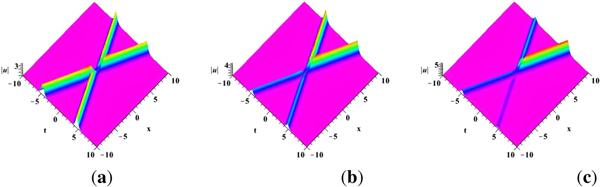
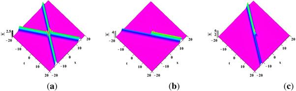
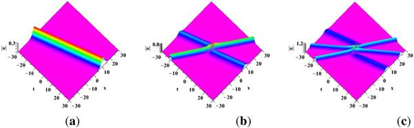
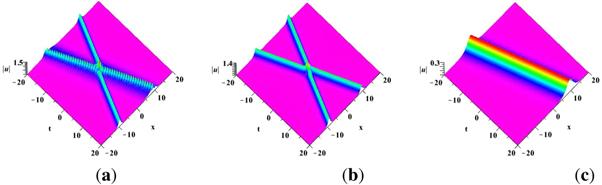
Now, we graphically illustrate the 2N1-soliton solution (67) with N1 = 1 in figure 1. By choosing three classes of parameters figures 12 display the propagation process of two-soliton on (x,t) plane. We let λ1 = 0.2 + 0.8i in figure 1. There is a crossing state of two solitons. If a11 = a21 = a31 = a41 = 0.4 + i is held, then one shows two solitons with the same amplitude. As shown in figure 1(b), if a11 = a21 = 0.4 + i, a31 = a41 = 0.4 is satisfied, the left and right sides of the solitons are asymmetric and the amplitude of the left side has declined significantly. We further let a21 = 0.4 + i, a11 = a31 = a41 = 0.4, three quarters of soliton decreases. Actually, this is different from figure 2. If we suppose a21 = a31 = a41 = 0 or a11 = a31 = a41 = 0, figures 2(b), (c) exhibits two single solitons with asymmetric shape. the two-soliton in figure 2(a) can be regarded as an incomplete superposition state of these two single solitons. That is a type of inelastic collision behavior. Since the eigenvalues λi, i = 1, 2, … for the N2-soliton solution are purely imaginary, thus we let λ1 = 0.3i, λ1 = 0.6i, λ1 = 0.45i in the solution (72) with N2 = 1, 2, 3. As shown in figure 3, there are one-, two- and three-soliton, which are similar to the 2N1-soliton. The latter can be regarded as the even order soliton. One can present an even number of solitons when N1 is chosen as any positive integer. As shown in figure 4, 2N1 + N2-soliton solution with N1 = N2 = 1 presents a degenerate process of soliton by setting suitable parameters. Especially, 4(a) shows a collision of the single soliton and two-soliton entanglement so-called bound state. However, if we take b11 = 0 and keep other parameter values, then there is a two-soliton keeping a crossing shape. Letting a11 = a12 = a13 = 0 in the solution only a single soliton is exhibited. This complete superposition process is similar to figure 2. Although three types of soliton solutions display the interaction behaviors of multi-soliton via suitable parameter values. For the first type of soliton solution, there exist inelastic collision behaviors when one changes some parameters. That is to say, they are incomplete superposition behaviors. Compared with the expressions of the 2N1-soliton solution and N2-soliton solution, we can find the latter is part of the former. The third type of soliton solution exhibits the combination of a single soliton and a two-soliton, in which a single soliton combines with one of the two-soliton to form a bound state. This result is different from the first two soliton solutions. If we increase the value of N2, 2N1 + N2-soliton solution can generate more bound solitons.

The nonlocal SS equation has the $2{N}_{1}+{N}_{2}$-soliton solution

$\begin{eqnarray*}\begin{array}{l}{u}_{2{N}_{1}+{N}_{2}}=2{\rm{i}}\displaystyle \sum _{k=1}^{{N}_{1}}\displaystyle \sum _{j=1}^{{N}_{1}}{a}_{1k}{{\rm{e}}}^{{\theta }_{k}-{\theta }_{j}^{* }}{\left({{\boldsymbol{M}}}^{-1}\right)}_{{kj}}\\ +2{\rm{i}}\displaystyle \sum _{k=1}^{{N}_{1}}\displaystyle \sum _{j={N}_{1}+1}^{2{N}_{1}}{a}_{1k}{{\rm{e}}}^{{\theta }_{k}-{\theta }_{j-{N}_{1}}(x,-t)}{\left({M}^{-1}\right)}_{{kj}}\\ +2{\rm{i}}\displaystyle \sum _{k=1}^{{N}_{1}}\displaystyle \sum _{j=2{N}_{1}+1}^{2{N}_{1}+{N}_{2}}{a}_{1k}{{\rm{e}}}^{{\theta }_{k}-{\theta }_{j-{N}_{1}}^{* }(x,-t)}{\left({{\boldsymbol{M}}}^{-1}\right)}_{{kj}}\\ +2{\rm{i}}\displaystyle \sum _{k={N}_{1}+1}^{2{N}_{1}}\displaystyle \sum _{j=1}^{{N}_{1}}{a}_{2,k-{N}_{1}}^{* }{{\rm{e}}}^{{\theta }_{k-{N}_{1}}^{* }(x,-t)-{\theta }_{j}^{* }}{\left({{\boldsymbol{M}}}^{-1}\right)}_{{kj}}\\ +2{\rm{i}}\displaystyle \sum _{k={N}_{1}+1}^{2{N}_{1}}\displaystyle \sum _{j={N}_{1}+1}^{2{N}_{1}}{a}_{2,k-{N}_{1}}^{* }{{\rm{e}}}^{{\theta }_{k-{N}_{1}}^{* }(x,-t)-{\theta }_{j-{N}_{1}}(x,-t)}{\left({{\boldsymbol{M}}}^{-1}\right)}_{{kj}}\\ +2{\rm{i}}\displaystyle \sum _{k=2{N}_{1}+1}^{2{N}_{1}+{N}_{2}}\displaystyle \sum _{j=2{N}_{1}+1}^{2{N}_{1}+{N}_{2}}{b}_{1,k-2{N}_{1}}{{\rm{e}}}^{{\theta }_{k}-{\theta }_{j}^{* }}{\left({{\boldsymbol{M}}}^{-1}\right)}_{{kj}}\end{array}\end{eqnarray*}$
$\begin{eqnarray}\begin{array}{l}+2{\rm{i}}\displaystyle \sum _{k=2{N}_{1}+1}^{2{N}_{1}+{N}_{2}}\displaystyle \sum _{j=1}^{{N}_{1}}{b}_{1,k-2{N}_{1}}{{\rm{e}}}^{{\theta }_{k}-{\theta }_{j}^{* }}{\left({{\boldsymbol{M}}}^{-1}\right)}_{{kj}}\\ +2{\rm{i}}\displaystyle \sum _{k=2{N}_{1}+1}^{2{N}_{1}+{N}_{2}}\displaystyle \sum _{j={N}_{1}+1}^{2{N}_{1}}{b}_{1,k-2{N}_{1}}{{\rm{e}}}^{{\theta }_{k}-{\theta }_{j-{N}_{1}}(x,-t)}{\left({{\boldsymbol{M}}}^{-1}\right)}_{{kj}}\\ +2{\rm{i}}\displaystyle \sum _{k={N}_{1}+1}^{2{N}_{1}}\displaystyle \sum _{j=2{N}_{1}+1}^{2{N}_{1}+{N}_{2}}{a}_{2,k-{N}_{1}}^{* }{{\rm{e}}}^{{\theta }_{k-{N}_{1}}^{* }(x,-t)-{\theta }_{j}^{* }}{\left({{\boldsymbol{M}}}^{-1}\right)}_{{kj}},\end{array}\end{eqnarray}$
where ${\boldsymbol{M}}={\left({m}_{{kj}}\right)}_{(2{N}_{1}+{N}_{2})\times (2{N}_{1}+{N}_{2})}$ with
$\begin{eqnarray}{m}_{{kj}}=\left\{\begin{array}{l}\displaystyle \frac{{{\rm{e}}}^{-{\theta }_{k}^{* }-{\theta }_{j}}+\displaystyle \sum _{\iota =1}^{4}{a}_{\iota k}^{* }{a}_{\iota j}{{\rm{e}}}^{{\theta }_{k}^{* }+{\theta }_{j}}}{{\lambda }_{j}-{\lambda }_{k}^{* }},1\leqslant k,j\leqslant {N}_{1},\\ \displaystyle \frac{{{\rm{e}}}^{-{\theta }_{k}^{* }-{\theta }_{j-{N}_{1}}^{* }(x,-t)}+{\eta }_{k,j-{N}_{1}}^{* }{{\rm{e}}}^{{\theta }_{k}^{* }+{\theta }_{j-{N}_{1}}^{* }(x,-t)}}{-{\lambda }_{j-{N}_{1}}^{* }-{\lambda }_{k}^{* }},1\leqslant k\leqslant {N}_{1},{N}_{1}+1\leqslant j\leqslant 2{N}_{1},\\ \displaystyle \frac{{{\rm{e}}}^{-{\theta }_{k}^{* }-{\theta }_{j}}+\displaystyle \sum _{\iota =1}^{4}{a}_{\iota k}^{* }{b}_{\iota ,j-2{N}_{1}}{{\rm{e}}}^{{\theta }_{k}^{* }+{\theta }_{j}}}{{\lambda }_{j}-{\lambda }_{k}^{* }},\,1\leqslant k\leqslant {N}_{1},\,2{N}_{1}+1\leqslant j\leqslant 2{N}_{1}+{N}_{2},\\ \displaystyle \frac{{{\rm{e}}}^{-{\theta }_{k-{N}_{1}}(x,-t)-{\theta }_{j}}+{\eta }_{j,k-{N}_{1}}{{\rm{e}}}^{{\theta }_{k-{N}_{1}}(x,-t)+{\theta }_{j}}}{{\lambda }_{j}+{\lambda }_{k-{N}_{1}}},{N}_{1}+1\leqslant k\leqslant 2{N}_{1},1\leqslant j\leqslant {N}_{1},\\ \displaystyle \frac{{{\rm{e}}}^{-{\theta }_{k-{N}_{1}}(x,-t)-{\theta }_{j-{N}_{1}}^{* }(x,-t)}+\displaystyle \sum _{\iota =1}^{4}{a}_{\iota ,k-{N}_{1}}{a}_{\iota ,j-{N}_{1}}^{* }{{\rm{e}}}^{{\theta }_{k-{N}_{1}}(x,-t)+{\theta }_{j-{N}_{1}}^{* }(x,-t)}}{-{\lambda }_{j-{N}_{1}}^{* }+{\lambda }_{k-{N}_{1}}},{N}_{1}+1\leqslant k,j\leqslant 2{N}_{1},\\ \displaystyle \frac{{{\rm{e}}}^{-{\theta }_{k-{N}_{1}}(x,-t)-{\theta }_{j}}+{\hat{\eta }}_{j-2{N}_{1},k-{N}_{1}}{{\rm{e}}}^{{\theta }_{k-{N}_{1}}(x,-t)+{\theta }_{j}}}{{\lambda }_{j}+{\lambda }_{k-{N}_{1}}},{N}_{1}+1\leqslant k\leqslant 2{N}_{1},2{N}_{1}+1\leqslant j\leqslant 2{N}_{1}+{N}_{2},\\ \displaystyle \frac{{{\rm{e}}}^{-{\theta }_{k}^{* }-{\theta }_{j}}+\displaystyle \sum _{\iota =1}^{4}{b}_{\iota ,k-2{N}_{1}}^{* }{a}_{\iota j}{{\rm{e}}}^{{\theta }_{k}^{* }+{\theta }_{j}}}{{\lambda }_{j}-{\lambda }_{k}^{* }},2{N}_{1}+1\leqslant k\leqslant 2{N}_{1}+{N}_{2},1\leqslant j\leqslant {N}_{1},\\ \displaystyle \frac{{{\rm{e}}}^{-{\theta }_{k}^{* }-{\theta }_{j-{N}_{1}}^{* }(x,-t)}+{\hat{\eta }}_{k-2{N}_{1},j-{N}_{1}}^{* }{{\rm{e}}}^{{\theta }_{k}^{* }+{\theta }_{j-{N}_{1}}^{* }(x,-t)}}{-{\lambda }_{j-{N}_{1}}^{* }-{\lambda }_{k}^{* }},2{N}_{1}+1\leqslant k\leqslant 2{N}_{1}+{N}_{2},{N}_{1}+1\leqslant j\leqslant 2{N}_{1},\\ \displaystyle \frac{{{\rm{e}}}^{-{\theta }_{k}^{* }-{\theta }_{j}}+\displaystyle \sum _{\iota =1}^{4}{b}_{\iota ,k-2{N}_{1}}^{* }{b}_{\iota ,j-2{N}_{1}}{{\rm{e}}}^{{\theta }_{k}^{* }+{\theta }_{j}}}{{\lambda }_{j}-{\lambda }_{k}^{* }},2{N}_{1}+1\leqslant k,j\leqslant 2{N}_{1}+{N}_{2},\\ {\hat{\eta }}_{r,s}={b}_{1r}{a}_{2,s}+{b}_{2r}{a}_{1,s}+{b}_{3r}{a}_{4,s}+{b}_{4r}{a}_{3,s},{\eta }_{r,s}={a}_{1r}{a}_{2,s}+{a}_{2r}{a}_{1,s}+{a}_{3r}{a}_{4,s}+{a}_{4r}{a}_{3,s}.\end{array}\right.\end{eqnarray}$
Also, $2{N}_{1}+{N}_{2}$-soliton solution can be reduced to the determinant form
$\begin{eqnarray}{u}_{2{N}_{1}+{N}_{2}}=2{\rm{i}}\displaystyle \frac{\det ({\boldsymbol{\Sigma }})}{\det ({\boldsymbol{M}})},\end{eqnarray}$
where ${\boldsymbol{\Sigma }}$ is given by
$\begin{eqnarray}{\boldsymbol{\Sigma }}=\left(\begin{array}{cc}0 & {{\boldsymbol{m}}}_{3}\\ {{\boldsymbol{n}}}_{3} & {{\boldsymbol{M}}}_{(2{N}_{1}+{N}_{2})\times (2{N}_{1}+{N}_{2})}\end{array}\right)\end{eqnarray}$
with
$\begin{eqnarray}\begin{array}{rcl}{{\boldsymbol{n}}}_{3} & = & \left({{\rm{e}}}^{-{\theta }_{1}^{* }},\ldots ,{{\rm{e}}}^{-{\theta }_{{N}_{1}}^{* }},{{\rm{e}}}^{-{\theta }_{1}(x,-t)},\ldots ,{{\rm{e}}}^{-{\theta }_{{N}_{1}}(x,-t)},\right.\\ & & {\left.{{\rm{e}}}^{-{\theta }_{2{N}_{1}+1}^{* }},\ldots ,{{\rm{e}}}^{-{\theta }_{2{N}_{1}+{N}_{2}}^{* }}\right)}^{{\rm{T}}},\\ {{\boldsymbol{m}}}_{3} & = & ({a}_{11}{{\rm{e}}}^{{\theta }_{1}},\ldots ,{a}_{1{N}_{1}}{{\rm{e}}}^{{\theta }_{{N}_{1}}},{a}_{21}^{* }{{\rm{e}}}^{{\theta }_{1}^{* }(x,-t)},\ldots ,{a}_{2{N}_{1}}^{* }{{\rm{e}}}^{{\theta }_{{N}_{1}}^{* }(x,-t)},\\ & & {b}_{11}{{\rm{e}}}^{{\theta }_{2{N}_{1}+1}},\ldots ,{b}_{1{N}_{2}}{{\rm{e}}}^{{\theta }_{2{N}_{1}+{N}_{2}}}).\end{array}\end{eqnarray}$

Figure 1. 2N1-soliton with N1 = 1, λ1 = 0.2 + 0.8i by choosing suitable parameters:(a) a11 = a21 = a31 = a41 = 0.4 + i, ; (b) a11 = a21 = 0.4 + i, a31 = a41 = 0.4; (c) a21 = 0.4 + i, a11 = a31 = a41 = 0.4.
Figure 2. 2N1-soliton with N1 = 1, λ1 = 0.4 + 0.8i by choosing suitable parameters:(a) a11 = a21 = a31 = a41 = 0.4 + i; (b) a11 = 0.4 + i, a21 = a31 = a41 = 0; (c) a21 = 0.4 + i, a11 = a31 = a41 = 0.4.
Figure 3. N2-soliton with N2 = 2 by choosing suitable parameters: b11 = b21 = b31 = b41 = b12 = b22 = b32 = b42 = b13 = b23 = b33 = b43, (a) λ1 = 0.3i, b11 = 0.6; (b) λ1 = 0.3i, λ2 = 0.6i, b11 = b12 = 0.6; (c) λ1 = 0.3i, λ2 = 0.6i, λ3 = 0.45i, b11 = b12 = b13 = 0.6.
Figure 4. (2N1 + N2)-soliton with N1 = N2 = 1 by choosing suitable parameters:λ1 = 0.5 + 0.8i, λ3 = 0.3i, a11 = a21 = a31 = a41, a12 = a22 = a32 = a42, a13 = a23 = a33 = a43, b11 = b21 = b31 = b41 (a) a11 = a12 = a13 = 0.4, b11 = 0.6; (b) a11 = a12 = a13 = 0.4, b11 = 0; (c) a11 = a12 = a13 = 0, b11 = 0.6.

5. Conclusions

In this work, the Riemann–Hilbert problem and the three types of soliton solutions for the physically meaningful nonlocal integrable Sasa–Satsuma equation have been studied. We constructed a single soliton solution of the nonlocal Sasa–Satsuma equation from the reduction of those of the local Sasa–Satsuma equation. Based on that, the multi-soliton solutions of the nonlocal Sasa–Satsuma equation have been constructed and verified by using an algebraic method. In order to explain the dynamic characteristics of soliton solutions better, some soliton dynamics were theoretically and graphically explored. The method presented in this work is a pure algebra method, which can be effectively used to study other nonlocal nonlinear integrable models and the dynamics of soliton collision.

Data availability statements

The data used to support the findings of this study are available from the corresponding author upon request.

Compliance with ethical standards

Conflict of interest

The authors declare that they have no conflict of interest.

The authors would like to thank the Editor and Reviewers for their valuable comments. The work of Y Chen was supported by the Fundamental Research Funds for the Central Universities (Grant No. 2022FRFK060015). The work of XW Yan was supported by the China Postdoctoral Science Foundation (Grant No. 2022M710969) and the National Natural Science Foundation of China (No. 12101159).

1
Valdmanis J A Fork R L Gordon J P 1985 Generation of optical pulses as short as 27 femtoseconds directly from a laser balancing self-phase modulation, group-velocity dispersion, saturable absorption, and saturable gain Opt. Lett. 10 131 133

DOI

2
Fork R L Shank C V Yen R Hirlimann C A 1983 Femtosecond optical pulses IEEE J. Quantum Elect. 19 500 506

DOI

3
Agrawal G P 2007 Nonlinear Fiber Optics New York Academic

4
Kodama Y 1985 Optical solitons in a monomode fiber J. Stat. Phys. 39 597 614

DOI

5
Kodama Y Hasegawa A 1987 Nonlinear pulse propagation in a monomode dielectric guide IEEE J. Quantum Elect. 23 510 524

DOI

6
Porsezian K Nakkeeran K 1996 Optical solitons in presence of Kerr dispersion and self-frequency shift Phys. Rev. Lett. 76 3955

DOI

7
Gedalin M Scott T C Band Y B 1997 Optical solitary waves in the higher order nonlinear Schrödinger equation Phys. Rev. Lett. 78 448

DOI

8
Sasa N Satsuma J 1991 New-type of soliton solutions for a higher-order nonlinear Schrödinger equation J. Phys. Soc. Japan 60 409 417

DOI

9
Nimmo J J C Yilmaz H 2015 Binary Darboux transformation for the Sasa–Satsuma equation J. Phys. A: Math. Theor. 48 425202

DOI

10
Xu J Fan E 2013 The unified transform method for the Sasa–Satsuma equation on the half-line Proc. R. Soc. A  469 20130068

DOI

11
Yang J Kaup D J 2009 Squared eigenfunctions for the Sasa–Satsuma equation J. Math. Phys. 50 023504

DOI

12
Mahalingam A Porsezian K 2002 Propagation of dark solitons in a system of coupled higher-order nonlinear Schrödinger equations J. Phys. A 35 3099 3109

DOI

13
Vinoj M N Kuriakose V C 2000 Multisoliton solutions and integrability aspects of coupled higher-order nonlinear Schrödinger equations Phys. Rev. E 62 8719 8725

DOI

14
Wu J P Geng X G 2017 Inverse scattering transform of the coupled Sasa–Satsuma equation by Riemann–Hilbert approach Commun. Theor. Phys. 67 527 534

DOI

15
Nakkeeran K Porsezian K Shanmugha Sundaram P Mahalingam A 1998 Optical solitons in coupled higher order nonlinear schrödinger equations Phys. Rev. Lett. 80 1425 1428

DOI

16
Wang D S Zhang D J Yang J 2010 Integrable properties of the general coupled nonlinear Schrödinger equations J. Math. Phys. 51 023510

DOI

17
Shepelsky D Zielinski L 2017 The inverse scattering transform in the form of a Riemann–Hilbert problem for the Dullin–Gottwald–Holm equation Opuscula Math. 37 167 187

DOI

18
Ma W X Huang Y Wang F 2020 Inverse scattering transforms and soliton solutions of nonlocal reverse-space nonlinear Schrödinger hierarchies Stud. Appl. Math. 145 563 585

DOI

19
Ma W X 2022 Riemann–Hilbert problems and inverse scattering of nonlocal real reverse-spacetime matrix AKNS hierarchies Phys. D 430 133078

DOI

20
Ma W X 2021 Riemann–Hilbert problems and soliton solutions of nonlocal real reverse-spacetime mKdV equations J. Math. Anal. Appl. 498 124980

DOI

21
Li Y Tian S F Yang J J 2022 Riemann–Hilbert problem and interactions of solitons in the-component nonlinear Schrödinger equations Stud. Appl. Math. 148 577 605

DOI

22
Ma W X 2019 Riemann-Hilbert problems and soliton solutions of a multicomponent mKdV system and its reduction Math. Methods Appl. Sci. 42 1099 1113

DOI

23
Yan X W 2020 Riemann–Hilbert method and multi-soliton solutions of the Kundu-nonlinear Schrödinger equation Nonlinear Dyn. 102 2811 2819

DOI

24
Wang X B Han B 2020 Application of the Riemann–Hilbert method to the vector modified Korteweg-de Vries equation Nonlinear Dyn. 99 1363 1377

DOI

25
Peng W Q Tian S F Wang X B Zhang T T 2019 Riemann–Hilbert method and multi-soliton solutions for three-component coupled nonlinear Schrödinger equations J. Geom. Phys. 146 103508

DOI

26
Ma W X 2018 Riemann–Hilbert problems of a six-component fourth-order AKNS system and its soliton solutions Comput. Appl. Math. 37 6359 6375

DOI

27
Tian S F 2017 Initial-boundary value problems for the general coupled nonlinear Schrödinger equation on the interval via the Fokas method J. Differ. Equ. 262 506 558

DOI

28
Tian S F 2017 Initial-boundary value problems of the coupled modified Korteweg-de Vries equation on the half-line via the Fokas method J. Phys. A 50 395204

DOI

29
Wazwaz A M 2004 Compacton solutions of higher order nonlinear dispersive KdV-like equations Appl. Math. Comput. 147 449 460

DOI

30
Wazwaz A M Xu G Q 2016 Negative-order modified KdV equations: multiple soliton and multiple singular soliton solutions Math. Methods Appl. Sci. 39 661 667

DOI

31
Wazwaz A M El-Tantawy S A 2017 Solving the (3+1)-dimensional KP-Boussinesq and BKP-Boussinesq equations by the simplified Hirota's method Nonlinear Dyn. 88 3017 3021

DOI

32
Fokas A S Lenells J 2012 The unified method: I. Nonlinearizable problems on the half-line J. Phys. A: Math. Theor. 45 195201

DOI

33
Zhao Z Han B 2017 Lie symmetry analysis, Bäcklund transformations, and exact solutions of a (2+1)-dimensional Boiti-Leon-Pempinelli system J. Math. Phys. 58 101514

DOI

34
Zhao Z 2019 Conservation laws and nonlocally related systems of the Hunter-Saxton equation for liquid crystal Anal. Math. Phys. 9 2311 2327

DOI

35
Zhao Z He L 2021 Lie symmetry, nonlocal symmetry analysis, and interaction of solutions of a (2+1)-dimensional KdV-mKdV equation Theor. Math. Phys. 206 142 162

DOI

36
Wang D S Wang X L 2018 Long-time asymptotics and the bright N-soliton solutions of the Kundu-Eckhaus equation via the Riemann–Hilbert approach Nonlinear Anal. 41 334 361

DOI

37
Xu J Fan E G 2015 Long-time asymptotics for the Fokas-Lenells equation with decaying initial value problem: without solitons J. Diff. Equ. 259 1098 1148

DOI

38
Lenells J 2012 Initial-boundary value problems for integrable evolution equations with 3 × 3 Lax pairs Phys. D: Nonlinear Phenom. D 241 857 875

DOI

39
Yang J 2018 Physically significant nonlocal nonlinear Schrödinger equation and its soliton solutions Phys. Rev. E 98 042202

DOI

40
Wang X B Han B 2021 The nonlinear steepest descent approach for long time behavior of the two-component coupled Sasa–Satsuma equation with a lax pair Taiwanese J. Math. 25 381 407

DOI

41
Liu L Tian B Yuan Y Q Du, Dark-bright Z 2018 solitons and semirational rogue waves for the coupled Sasa–Satsuma equations Phys. Rev. E 97 052217

DOI

42
Zhang H Q Wang Y Ma W X 2017 Binary Darboux transformation for the coupled Sasa–Satsuma equations Chaos 27 073102

DOI

43
Geng X Chen M Wang K 2021 Application of the nonlinear steepest descent method to the coupled Sasa–Satsuma equation East J. Appl. Math. 11 181 206

DOI

44
Xu T Xu X M 2013 Single- and double-hump femtosecond vector solitons in the coupled Sasa–Satsuma system Phys. Rev. E 87 032913

DOI

45
Song C Xiao D Zhu Z 2017 Reverse space-time nonlocal Sasa–Satsuma equation and its solutions J. Phys. Soc. Japan 86 054001

DOI

Outlines

/