


1. Introduction
Nonlinear partial differential equations (NLPDEs) are the result of the mathematical modelling of physical problems. NLPDEs have been associated with many innovative projects over the last decades. Researchers and mathematicians have done amazing work in constructing new methods and techniques for calculating analytical solutions for NLPDEs. In the recent decade, much attention has been paid to investigating solitary wave solutions for NLPDEs. Soliton theory has vast applications in the fields of biophysics, quantum mechanics, nonlinear optics, microbiology, and engineering. A soliton is a packet of waves that reinforces itself and keeps its form while it travels at a steady speed. Solitons are in the form of solitary waves that act like particles when they move with constant velocity. The solitary waves occur in many circumstances, including the description of water waves and the propagation of light in optical fibers. Nowadays, with the fast development in symbolic calculations, the study of soliton solutions to nonlinear evolution equations has attracted the attention of many researchers. It has brought a revolution in advanced mathematical physics, steady-state physics, and telecommunication systems. The wave propagation in a dynamical system is described by a wide range of physical models.
Many studies have been conducted that offer precise and closed form solutions to the NLPDEs. For finding exact solutions of NLPDEs, a wide variety of sophisticated mathematical techniques have been established that include the exp-function method [1], the variational method [2], the auxiliary differential equation method [3], the tanh method [4], the $\left(\tfrac{{G}^{{\prime} }}{G}\right)$-expansion method [5], the Jacobi elliptic function expansion method [6], the function transformation method [7], F-expansion methods [8], the local weak form meshless technique [9], the first integral method [10], the homotopy perturbation method [11], the sine-Gordon expansion method [12], the generalized Kudryashov method [13], the exponential rational function method [14], the modified Kudryashov method [15], and modified simple equation method [16], etc. These techniques are used for extracting new solitary wave solutions to NLPDEs.
A shallow water ocean wave is a surface wave that is influenced by the ocean floor. These waves assemble when the surface of the water is ruffled by external forces such as wind, gravity, earthquakes, or landslides on the ocean’s bottom. When a wave travels across an area of water, the gravitational pull of the Earth, or in the case of the tiniest ripples, the surface tension of the water, will pull the water back to its original state. A perfect ocean wave pattern may be characterized by many parameters such as length, height, period, and speed. These features are dictated by the mechanisms that create the wave, as well as the wave’s contact with the ocean bottom in shallow-water waves (SWWs). These wave patterns are studied by finding soliton solutions to the nonlinear model. These solitons are often discretized by the shallow water dynamics seen on ocean lakes, canals, and beaches.
Numerous forms of NLEEs are used to explain SWWs, such as the Korteweg–de Vries equation for long shallow water gravity waves [17], the Boussinesq-Burgers system for SWWs on an ocean beach or in a lake [18], and the perturbed Boussinesq equation (PBE) for the solution interaction mechanism of SWWs. All of these equations have one thing in common, they all accommodate soliton solutions.
The PBE is one of the crucial mathematical models [19] used for describing nonlinear phenomena that has nonlinearity and dispersion of fourth order. The mathematical expression for PBE can be seen in [19, 20].1.1 ) the wave pattern is indicated by h(x, t), whereas the independent variables t and x are the temporal and spatial correlatives, respectively. Where Σ is the dissipation coefficient and δ serves as the higher order stabilization term also l, m and s are all constant [21]. The coefficient of the nonlinear term is represented by m on the left side of equation (1.1 ). Typically, n determines the degree of nonlinearity. Soliton solutions are generated from equation (1.1 ). These solitons result from a precise balance of dispersion and nonlinear effects. Solitons are confined waves that travel without changing their velocity and shape attributes and are steady against periodic collisions [22]. Specifically, a single wave that resembles the appearance of elastic or particle waves is called a soliton. In coastal engineering, the perturbed Boussinesq equation is frequently employed. In this study, we’ll look at the dynamics of SWWs as they are simulated using the Boussinesq equation with significant perturbation terms.
$\begin{eqnarray}\begin{array}{l}{h}_{{tt}}-{l}^{2}{h}_{{xx}}+m{\left({h}^{2n}\right)}_{{xx}}+{{sh}}_{{xxxx}}\\ \,\,=\,\sigma {h}_{{xx}}+\delta {h}_{{xxxx}}.\end{array}\end{eqnarray}$
Here, in equation (In this article, the PBE is investigated using the two most efficient and reliable methodologies such as the unified method and the singular manifold method. The singular manifold method is an extension of Painlevé analysis. Using the singular manifold technique, we have been able to solve for singular soliton solutions. The unified technique is one of the most truthful, practical, and accessible algebraic approaches for extracting exact solutions to NLEEs. This method allows the researcher to acquire the traveling wave solutions in two different forms: polynomial function solutions and rational solutions. In addition, the Painlevé test has been used to examine the integrability of the suggested model.
The paper is organised as follows. Section 2 includes a brief discussion of suggested techniques; the singular manifold method and the unified method. The algorithm of Painlevé integrability test is also discussed in this section. In section 3 , we provide a mathematical description of the suggested model. Section 4 provides the applications of proposed methodologies to the governing model. In section 5 , the integrability of the proposed model is investigated via the Painlevé test. Section 5 is based on the results and discussions. Section 6 features the conclusion.
2. Interpretation of suggested techniques
In this section, the suggested methods, including the singular manifold method (SMM) and the unified method (UM) have been discussed in detail. The algorithm of the Painlevé test has also been discussed in detail.
Consider the following nonlinear partial differential equation as
$\begin{eqnarray}\gamma (h,\,{h}_{x},\,{h}_{t},\,{h}_{{xx}},\,{h}_{{xt}},\,{h}_{{tt}}...),\end{eqnarray}$
whose ODE form is as follows, $\begin{eqnarray}\xi (u,{u}^{{\prime} },-\vartheta {u}^{{\prime} },{u}^{{\prime\prime} },-\vartheta {u}^{{\prime\prime} },-{\vartheta }^{2}{u}^{{\prime\prime} }...),\end{eqnarray}$
using the traveling wave transformation η = x − ϑt, where ϑ represents the speed of a wave.2.1. Method 1: the singular manifold method
This subsection includes a brief overview of the singular manifold approach.
Step 1. The singular manifold method [23, 24] is used to asset innovative analytical solutions to NLPDEs. The Painlevé test, developed by Weiss [24], is the foundation of SMM. The solution of equation (2.2 ) is specified as follows:
$\begin{eqnarray}u(\eta )=\displaystyle \sum _{j=0}^{\infty }{u}_{j}\psi {\left(\eta \right)}^{j-\alpha }.\end{eqnarray}$
Where ψ(η) is an eigenfunction that weights the poles and α is the predicted order of the poles determined by a dominant behavior analysis. It’s clear that there’s no singularity at j > α, thus the series must end there. When the series ends, it will be a Bäcklund truncated series.Step 2. When the coefficients of various powers of ψ are set to zero, an algebraic equation system is formed. By addressing this system, we may derive a Schwarzian derivative of the form
$\begin{eqnarray}{\left(\displaystyle \frac{\psi ^{\prime\prime} }{\psi ^{\prime} }\right)}^{{\prime} }-\displaystyle \frac{1}{2}{\left(\displaystyle \frac{\psi ^{\prime\prime} }{\psi ^{\prime} }\right)}^{2}=[\psi ,\eta ].\end{eqnarray}$
Step 3. The wave function ψ(η) is retrogradely substituted in equation (2.3 ), resulting in a solution comprising hyperbolic and trigonometric functions.
2.2. Method 2: unified method
The acquired solution of equation (2.2 ) through UM is characterized as the polynomial function solutions and the rational function solutions. This subsection incorporates a compact outline of a unified method [25].
Step 1. The polynomial function solutions
The polynomial functions satisfying equation (2.2 ), as proposed by UM, have the following form:2.5 ) satisfies the equation (2.2 ). A balancing strategy between the highest order linear and nonlinear components is necessary to get the exact values of n and k in equation (2.2 ) [26].
$\begin{eqnarray}\begin{array}{l}u(\eta )=\displaystyle \sum _{i=0}^{n}{p}_{i}{\psi }^{i}(\eta ),\\ {\left({\psi }^{{\prime} }(\eta )\right)}^{\nu }=\displaystyle \sum _{i=0}^{\nu k}{q}_{i}{\psi }^{i}(\eta ),\quad \eta =x-\vartheta t.\\ i=1,2,3,\ldots .\quad \nu =1,2,\end{array}\end{eqnarray}$
where qi and pi are constants to be determined and the solution obtained by equation (Step 2. Rational function solutions
According to UM, equation (2.2 ) has a rational solution as,2.2 ) [26] requires that the values of n and k be determined by striking a balance between the highest order linear and nonlinear components.
$\begin{eqnarray}\begin{array}{l}u(\eta )=\displaystyle \frac{{\sum }_{i=0}^{n}{a}_{i}{\psi }^{i}(\eta )}{{\sum }_{i=0}^{r}{c}_{i}{\psi }^{i}(\eta )},\quad n\geqslant r,\\ {\left({\psi }^{{\prime} }(\eta )\right)}^{\nu }=\displaystyle \sum _{i=0}^{\nu k}{b}_{i}{\psi }^{\nu }(\eta ).\quad \nu =1,2,\end{array}\end{eqnarray}$
where ai, ci and bi are constants to be evaluated. Equation (2.3. Painlevé test
The Painlevé test aims to determine whether or not NPDEs are integrable.
Step 1. First, investigate the dominant behavior by substituting2.1 ). λ represents the arbitrary parameter and c denotes the dominant behavior which is to be assessed at first. Then, we assume2.8 ) which has been calculated above. The value of h0(x, t) is obtained by putting the least power of ϱ(x, t) to zero.
$\begin{eqnarray}h(x,t)=\lambda {\varrho }^{c}(x,t),\end{eqnarray}$
into ( $\begin{eqnarray}h(x,t)={h}_{0}(x,t){\varrho }^{c}(x,t),\end{eqnarray}$
and substitute the value of c in equation (Step 2. The resonances corresponding to the dominant behavior are then computed by supposing2.9 ) into equation (2.2 ).
$\begin{eqnarray}h(x,t)={h}_{0}(x,t){\varrho }^{c}(x,t)+\displaystyle \sum _{k=1}^{\infty }{h}_{k}{\varrho }^{k+c}.\end{eqnarray}$
Putting equation (Step 3. The Painlevé test contains a compatibility criteria in which the coefficient hk(x, t) must match the resonance values that would originate from an arbitrary function. If the compatibility objectives are fulfilled at the resonance values, then equation (2.2 ) satisfies the painlevé test and is painlevé integrable.
3. Applications of proposed methods
In this section, there are two integrating techniques. The singular manifold technique and the unified method are applied to the proposed model for obtaining new and novel soliton solutions.
The following traveling wave transformation is required to implement the proposed methods.3.1 ), the governing model is converted into the following ODE3.2 ) twice yields the following equation as3.3 ).
$\begin{eqnarray}h(x,t)=u(\eta );\,\,\,\eta =x-\vartheta t\end{eqnarray}$
has been used. By the application of equation ( $\begin{eqnarray}\vartheta u^{\prime\prime} -{l}^{{2}u^{\prime\prime}} +m({u}^{2})^{\prime\prime} +{su}^{\prime\prime\prime\prime} =\sigma u^{\prime\prime} +\delta u^{\prime\prime\prime\prime} .\end{eqnarray}$
Integrating equation ( $\begin{eqnarray}({\vartheta }^{2}-{l}^{2}-\sigma )u+{{mu}}^{2}+(s-\delta )u^{\prime\prime} =0,\end{eqnarray}$
where dashes represent the derivative concerning η. For the purpose of deriving solutions of the suggested model, we have addressed the use of equation (3.1. Interrogate solution using the SMM
In this subsection, SMM [23, 24] is used to find out the new exact soliton solution for PBE. According to SMM, the solution of equation (3.3 ) is expressed in the form of a series which is based on the Painlevé analysis given by Weiss [24] as3.4 ) takes the following form3.5 ) in equation (3.3 ) and associating the various powers of ψ equals to zero results in a set of equations as shown below:3.10 ) into equation (3.5 ), we obtain3.11 ) into equation (3.9 ), after simplification we get3.13 ) in equation (3.11 ) and observing the relationship between u(η) and h(x, t) mentioned in equation (3.1 ), we get the solutions of the proposed model as given below3.14 ) is plotted in figures 1–2 by taking different values of arbitrary parameters.
$\begin{eqnarray}u(\eta )=\displaystyle \sum _{j=0}^{\infty }{u}_{j}\psi {\left(\eta \right)}^{j-\alpha },\end{eqnarray}$
whereas, α provides the predicted order of the poles based on a dominant behavior inspection and ψ is an eigenfunction that calculates the weights of the poles. The above series will be truncated when j = α. The dominating behavior yields α = 2. Equation ( $\begin{eqnarray}u(\eta )=\displaystyle \frac{{u}_{0}}{{\psi }^{2}}+\displaystyle \frac{{u}_{1}}{\psi }+{u}_{2}.\end{eqnarray}$
This is Bäcklund’s truncated series. Plugging equation ( $\begin{eqnarray}{\psi }^{-4}\,:\qquad 6(s-\delta ){u}_{0}{\left(\psi ^{\prime} \right)}^{2}+{{mu}}_{0}^{2}=0,\end{eqnarray}$
$\begin{eqnarray}\begin{array}{l}{\psi }^{-3}\,:\qquad 2(s-\delta )\left({u}_{1}{\left(\psi ^{\prime} \right)}^{2}-2{u}_{0}^{{\prime} }\psi ^{\prime} -{u}_{0}\psi ^{\prime\prime} \right)\\ \,+\,2{{mu}}_{0}{u}_{1}=0,\end{array}\end{eqnarray}$
$\begin{eqnarray}\begin{array}{l}{\psi }^{-2}\,:\qquad (s-\delta )\left({u}_{0}^{{\prime\prime} }-2{u}_{1}^{{\prime} }\psi ^{\prime} -{u}_{1}\psi ^{\prime\prime} \right)\\ \quad +({\vartheta }^{2}-{l}^{2}-\sigma ){u}_{0}+{{mu}}_{1}^{2}+2{{mu}}_{0}{u}_{2}=0,\end{array}\end{eqnarray}$
$\begin{eqnarray}{\psi }^{-1}\,:\qquad (s-\delta ){u}_{1}^{{\prime\prime} }+({\vartheta }^{2}-{l}^{2}-\sigma ){u}_{1}+2{{mu}}_{1}{u}_{2}=0.\end{eqnarray}$
Solving the above equations yields; $\begin{eqnarray}\begin{array}{l}{u}_{0}=-\displaystyle \frac{6}{m}(s-\delta ){\left({\psi }^{{\prime} }\right)}^{2},\\ {u}_{1}=\displaystyle \frac{6}{m}(s-\delta ){\psi }^{{\prime\prime} },\\ {u}_{2}=-\displaystyle \frac{1}{2}\displaystyle \frac{({\vartheta }^{2}-{l}^{2}-\sigma )}{m}-\displaystyle \frac{1}{2}\displaystyle \frac{(s-\delta )}{m}\\ \times \left(4\left(\displaystyle \frac{{\psi }^{\prime\prime\prime }}{{\psi }^{{\prime} }}\right)-3{\left(\displaystyle \frac{{\psi }^{{\prime\prime} }}{{\psi }^{{\prime} }}\right)}^{2}\right).\end{array}\end{eqnarray}$
Plugging equation ( $\begin{eqnarray}u(\psi )=\displaystyle \frac{6}{m}(s-\delta ){\left(\mathrm{ln}(\psi )\right)}^{{\prime\prime} }+{u}_{2}.\end{eqnarray}$
Now plugging equation ( $\begin{eqnarray}{\left(\displaystyle \frac{\psi ^{\prime\prime} }{\psi ^{\prime} }\right)}^{{\prime} }-\displaystyle \frac{1}{2}{\left(\displaystyle \frac{\psi ^{\prime\prime} }{\psi ^{\prime} }\right)}^{2}={d}_{1}.\end{eqnarray}$
That’s the Schwarzian derivative of the ψ eigenfunction. If we integrate the Schwarzian derivative of the eigenfunction ψ, we get its value as $\begin{eqnarray}\psi (\eta )={d}_{3}+\sqrt{\displaystyle \frac{2}{{d}_{1}}}{d}_{2}\tan \left(\sqrt{\displaystyle \frac{{d}_{1}}{2}}(\eta +2{d}_{4})\right).\end{eqnarray}$
Putting equation ( $\begin{eqnarray}\begin{array}{l}{h}_{1}(x,t)=-\displaystyle \frac{({\vartheta }^{2}-{l}^{2}-\sigma )-2{d}_{1}(s-\delta )}{2m}\times \left[1-\displaystyle \frac{3(2{d}_{2}^{2}+{d}_{1}{d}_{3}^{2})}{{\left[\sqrt{{d}_{1}}{d}_{3}\cos \left(\tfrac{\sqrt{{d}_{1}}(x-\vartheta t)+2{d}_{4}}{\sqrt{2}}\right)+\sqrt{2}{d}_{2}\sin \left(\tfrac{\sqrt{{d}_{1}}(x-\vartheta t)+2{d}_{4}}{\sqrt{2}}\right)\right]}^{2}}\right].\end{array}\end{eqnarray}$
equation (
Figure 1. Dynamical behavior of equation ( |
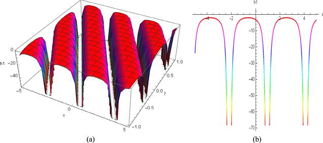
Figure 2. Dynamical behavior of equation ( |
3.2. Interrogate solutions using UM
In this section, the polynomial and rational solutions for equation (1.1 ) have been obtained using the unified method.
3.2.1. The polynomial solutions
Assume the suggested model’s polynomial solutions have the following form3.3 ), we use homogeneous balancing between u2 and u″. From this, we can calculate n = 2(k −1), where k is an integer i.e; k = 2, 3, 4... By taking k = 2, we obtain solutions corresponding to ν = 1 and ν = 2. As a result, we assume that the polynomial solution of the equation (3.3 ) takes the form,
$\begin{eqnarray}\begin{array}{l}u(\eta )=\displaystyle \sum _{i=0}^{n}{p}_{i}{\psi }^{i}(\eta ),\\ {\left({\psi }^{{\prime} }(\eta )\right)}^{\nu }=\displaystyle \sum _{i=0}^{\nu k}{q}_{i}{\psi }^{i}(\eta ).\quad \nu =1,2.\end{array}\end{eqnarray}$
pi and qi are unknown constants. In equation ( $\begin{eqnarray}\begin{array}{l}u(\eta )={p}_{0}+{p}_{1}\psi (\eta )+{p}_{2}{\psi }^{2}(\eta ),\\ {\left({\psi }^{{\prime} }(\eta )\right)}^{\nu }=\displaystyle \sum _{i=0}^{2\nu }{q}_{i}{\psi }^{i}(\eta ).\,\,\,\,\nu =1,2.\end{array}\end{eqnarray}$
(a) The solitary wave solutions:
The solitary wave solutions can be obtained by putting ν = 1 in equation (3.16 ), as3.17 ) into equation (3.3 ) and comparing the coefficients of ψ(η) equals zero. By solving this algebraic system of equations, we may determine the values of arbitrary constants, which we denote by1.1 ) is as follows3.19 ) is plotted in figure 3 by taking different values of arbitrary parameters.
$\begin{eqnarray}\begin{array}{l}u(\eta )={p}_{0}+{p}_{1}\psi (\eta )+{p}_{2}{\psi }^{2}(\eta ),\\ {\psi }^{{\prime} }(\eta )={q}_{0}+{q}_{1}\psi (\eta )+{q}_{2}{\psi }^{2}(\eta ).\end{array}\end{eqnarray}$
An algebraic system is obtained by substituting equation ( $\begin{eqnarray}\begin{array}{l}{q}_{0}=\displaystyle \frac{1}{4}\displaystyle \frac{(s-\delta )\,{q}_{1}^{2}+({\vartheta }^{2}-{l}^{2}-\sigma )}{{b}_{2}\,(s-\delta )},\\ {p}_{0}=-\displaystyle \frac{3}{2}\displaystyle \frac{{q}_{1}^{2}\,(s-\delta )+({\vartheta }^{2}-{l}^{2}-\sigma )}{m}\\ {p}_{1}=-\displaystyle \frac{6\,{q}_{1}\,{q}_{2}\,(s-\delta )}{m},\\ {p}_{2}=-\displaystyle \frac{6\,{q}_{2}^{2}\,(s-\delta )}{m},\\ {q}_{1}={q}_{1},\quad {q}_{2}={q}_{2}.\end{array}\end{eqnarray}$
The obtained solution of equation ( $\begin{eqnarray}\begin{array}{rcl}{h}_{2}(x,t) & = & -\displaystyle \frac{3}{2}\,\displaystyle \frac{({\vartheta }^{2}-{l}^{2}-\sigma )}{m}\\ & & \times \,\sec h\left(\displaystyle \frac{1}{2}\sqrt{\displaystyle \frac{{l}^{2}-{\vartheta }^{2}+\sigma }{s-\delta }}(x-\vartheta t)\right),\end{array}\end{eqnarray}$
where η = x −ϑt. Equation (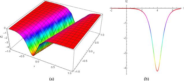
Figure 3. Dynamical behavior of equation ( |
(b) The soliton solutions:
The soliton solutions can be retrieved by plugging ν = 2 into the auxiliary equation given by equation (3.16 ). For ν = 2, the solution looks like this:3.20 ) into equation (3.3 ) and using the suggested procedure as explained above. The following values of arbitrary constants can be obtained as1.1 ):
$\begin{eqnarray}\begin{array}{l}u(\eta )={p}_{0}+{p}_{1}\psi (\eta )+{p}_{2}{\psi }^{2}(\eta ),\\ {\psi }^{{\prime} }(\eta )=\psi (\eta )\,\sqrt{{q}_{0}+{q}_{1}\psi (\eta )+{q}_{2}{\psi }^{2}(\eta )}.\end{array}\end{eqnarray}$
Putting equation ( $\begin{eqnarray}\begin{array}{l}{q}_{0}=\displaystyle \frac{({\vartheta }^{2}-{l}^{2}-\sigma )}{(s-\delta )},\quad {q}_{1}={q}_{1},\\ {q}_{2}=\displaystyle \frac{1}{4}\,\displaystyle \frac{{q}_{1}^{2}\,(s-\delta )}{({\vartheta }^{2}-{l}^{2}-\sigma )},\,{p}_{0}=-\displaystyle \frac{({\vartheta }^{2}-{l}^{2}-\sigma )}{m},\\ {p}_{1}=-\displaystyle \frac{3\,{q}_{1}\,(s-\delta )}{m},\,\,\,\,{p}_{2}=-\displaystyle \frac{3}{2}\,\displaystyle \frac{{q}_{1}^{2}\,{\left(s-\delta \right)}^{2}}{({\vartheta }^{2}-{l}^{2}-\sigma )},\,\,\,n=2.\end{array}\end{eqnarray}$
Here is the answer to equation ( $\begin{eqnarray}\begin{array}{rcl}{h}_{3}(x,t) & = & \displaystyle \frac{-12\,({e}^{\eta \,{R}_{2}})\,({\vartheta }^{2}-{l}^{2}-\sigma )\,{q}_{1}}{({e}^{{C}_{1}\,{R}_{2}})\left(\tfrac{{\left({e}^{\eta \,{R}_{2}}\right)}^{2}}{{\left({e}^{{C}_{1}\,{R}_{2}}\right)}^{2}}-\tfrac{2\,{q}_{1}\,{e}^{\eta \,{R}_{2}}}{{e}^{{C}_{1}\,{R}_{2}}}\right)\,m}\\ & & \times \left[\displaystyle \frac{2\,({e}^{\eta \,{R}_{2}})\,{q}_{1}}{({e}^{{C}_{1}\,{R}_{2}})\,\left(\tfrac{{\left({e}^{\eta \,{R}_{2}}\right)}^{2}}{{\left({e}^{{C}_{1}\,{R}_{2}}\right)}^{2}}-\tfrac{2\,{q}_{1}\,{e}^{\eta \,{R}_{2}}}{{e}^{{C}_{1}\,{R}_{2}}}\right)}+1\,\right]+{R}_{1},\end{array}\end{eqnarray}$
where η = x −ϑt, ${R}_{2}=\sqrt{\tfrac{{\vartheta }^{2}-{l}^{2}-\sigma }{s-\delta }}$ and ${R}_{1}=-\tfrac{{\vartheta }^{2}-{l}^{2}-\sigma }{m}$.(c) The elliptic wave solutions:
For ν = 2, the solution can be written as3.23 ) into equation (3.3 ). When the coefficients of ψ(η) are compared to zero, an algebraic system of equations is generated. By solving this set of equations, we may determine the values of arbitrary constants, which we denote by1.1 ) leads to the following form
$\begin{eqnarray}\begin{array}{l}u(\eta )={p}_{0}+{p}_{1}\psi (\eta )+{p}_{2}{\psi }^{2}(\eta ),\\ {\psi }^{{\prime} }(\eta )=\sqrt{{q}_{0}+{q}_{2}{\psi }^{2}(\eta )+{q}_{4}{\psi }^{4}(\eta )}.\end{array}\end{eqnarray}$
Substituting equation ( $\begin{eqnarray}\begin{array}{l}\sigma =-4\,\left(\sqrt{-3\,{q}_{0}\,{q}_{4}+{q}_{2}^{2}}\right)\,(s-\delta )-{l}^{2}+{\vartheta }^{2}\\ {q}_{2}={q}_{2},\,\,\,{q}_{4}={q}_{4},\\ {p}_{0}=-\displaystyle \frac{1}{2}\,\displaystyle \frac{4\,(s-\delta )\,{q}_{2}+({\vartheta }^{2}-{l}^{2}-\sigma )}{m},\\ {p}_{1}=0,\,\,\,\,{p}_{2}=-\displaystyle \frac{6\,{q}_{4}\,(s-\delta )}{m},\,\,\,n=2.\end{array}\end{eqnarray}$
In Jacobi elliptic functions, distinct solutions are obtained for different values of qi. The classification scheme in [27], gives $\begin{eqnarray}\begin{array}{l}{q}_{4}=-\displaystyle \frac{1}{4},\,\,\,{q}_{2}=\displaystyle \frac{1+{\gamma }^{2}}{2},\\ {q}_{0}=-\displaystyle \frac{{\left(1-{\gamma }^{2}\right)}^{2}}{2};\,\,\,0\lt \,\gamma \,\lt 1.\end{array}\end{eqnarray}$
The auxiliary equation becomes $\psi (\eta )=\gamma \,{cn}(\eta ,\gamma )\,+{dn}(\eta ,\gamma )$ and the solution to equation ( $\begin{eqnarray}\begin{array}{l}{h}_{4}(x,t)=-\displaystyle \frac{(s-\delta )\left({\gamma }^{2}-\tfrac{3}{2}{\left(\gamma \,{cn}(\eta ,\gamma )+{dn}(\eta ,\gamma )\right)}^{2}+\,2\,\sqrt{-\tfrac{1}{8}\,{\gamma }^{4}+\tfrac{5}{4}\,{\gamma }^{2}-\tfrac{1}{8}}+1\right)}{m}.\end{array}\end{eqnarray}$
The Jacobi elliptic functions have a modulus of γ (0 < γ < 1), where γ is an irrational number. When γ → 0, ${cn}(\eta )$, ${dn}(\eta )$ and ${sn}(\eta )$ deteriorate to $\cos (\eta )$, 1 and $\sin (\eta )$ respectively. While γ → 1, ${cn}(\eta )$, ${dn}(\eta )$ and ${sn}(\eta )$ degenerate to ${\rm{sech}} (\eta )$, ${\rm{sech}} (\eta )$ and $\tanh (\eta )$ respectively.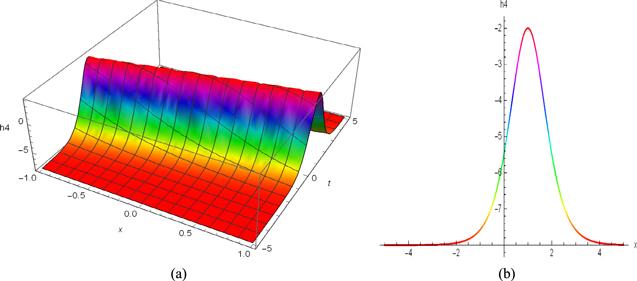
Figure 4. Dynamical behavior of equation ( |
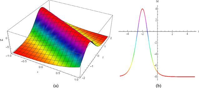
Figure 5. Dynamical behavior of equation ( |
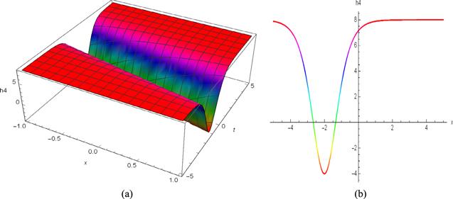
Figure 6. Dynamical behavior of equation ( |
3.2.2. The rational solutions
Suppose that the rational solutions for the proposed model have the following form 3.3 ). We have n −r = 2(k −1); k = 1, 2, 3,… When k = 1, we obtain n = r. The rational solutions can be found by taking ν = 2 and k = 1. As a consequence of equation (3.27 ), two features arise:
$\begin{eqnarray}\begin{array}{l}u(\eta )=\displaystyle \frac{{\sum }_{i=0}^{n}{a}_{i}{\psi }^{i}(\eta )}{{\sum }_{i=0}^{r}{c}_{i}{\psi }^{i}(\eta )},\quad n\geqslant r\\ {\left({\psi }^{{\prime} }(\eta )\right)}^{\nu }=\displaystyle \sum _{i=0}^{\nu k}{b}_{i}{\psi }^{i}(\eta ).\end{array}\end{eqnarray}$
the unknowns ai, bi and ci are constants. By taking the homogeneous balancing between u2 and u″ in equation ((a) Periodic rational solutions:
The periodic rational solutions can be obtained by putting ν = 2 in equation (3.27 ), as3.28 ) into equation (3.3 ), and comparing the coefficients of ψ(η) equals zero, yields an algebraic system of equations. By solving this set of equations, we may determine the values of arbitrary constants, which we denote by
$\begin{eqnarray}\begin{array}{l}u(\eta )=\displaystyle \frac{{a}_{0}+{a}_{1}\psi (\eta )}{{c}_{0}+{c}_{1}\psi (\eta )},\\ {\psi }^{{\prime} }(\eta )=\sqrt{{b}_{0}^{2}-{b}_{2}^{2}{\psi }^{2}(\eta )}.\end{array}\end{eqnarray}$
Plugging equation ( $\begin{eqnarray}\begin{array}{l}{b}_{0}=\displaystyle \frac{{c}_{0}\,\sqrt{\tfrac{{\vartheta }^{2}-{l}^{2}-\sigma }{s-\delta }}}{{c}_{1}},\,\,\,\,{b}_{2}=\sqrt{\displaystyle \frac{{\vartheta }^{2}-{l}^{2}-\sigma }{s-\delta }},\\ {a}_{0}=-\displaystyle \frac{3\,{c}_{0}({\vartheta }^{2}-{l}^{2}-\sigma )}{m},\\ {a}_{1}=0,\,\,{c}_{0}={c}_{0},\,\,{c}_{1}={c}_{1},\,\,n=2.\end{array}\end{eqnarray}$
The obtained solutions of equation (1.1 ) are as follows3.30 ) is plotted in figures 7 and 8 by taking different values of arbitrary parameters.
$\begin{eqnarray}{h}_{5}(x,t)=\displaystyle \frac{3\,{c}_{0}\,({\vartheta }^{2}-{l}^{2}-\sigma )\,{b}_{2}}{m\,\left(\sin \left({b}_{2}(-\eta +M)\right)\,{b}_{0}\,{c}_{1}-{c}_{0}\,{b}_{2}\right)},\end{eqnarray}$
where η = x −ϑt. Equation (
Figure 7. Dynamical behavior of equation ( |
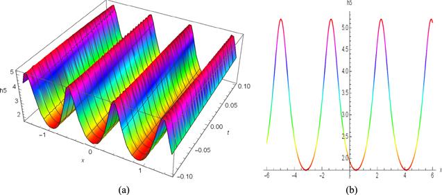
Figure 8. Dynamical behavior of equation ( |
(b) Soliton rational solutions:
The soliton rational solutions can be retrieved by plugging ν = 2 into the auxiliary equation given by equation (3.27 ). For ν = 2, the solution takes the following form3.31 ) into equation (3.3 ) and using the suggested method as explained above. The following values of arbitrary constants can be obtained as
$\begin{eqnarray}\begin{array}{l}u(\eta )=\displaystyle \frac{{a}_{0}+{a}_{1}\psi (\eta )}{{c}_{0}+{c}_{1}\psi (\eta )},\\ {\psi }^{{\prime} }(\eta )=\sqrt{{b}_{0}+{b}_{1}\psi (\eta )+{b}_{2}{\psi }^{2}(\eta )}.\end{array}\end{eqnarray}$
Plugging equation ( $\begin{eqnarray}\begin{array}{l}{b}_{0}=\displaystyle \frac{{c}_{0}^{2}\,({\vartheta }^{2}-{l}^{2}-\sigma )+{c}_{1}\,{c}_{0}\,{b}_{1}\,(s-\delta )}{{c}_{1}^{2}(s-\delta )},\\ {b}_{1}={b}_{1},\,\,\,\,{b}_{2}=-\displaystyle \frac{({\vartheta }^{2}-{l}^{2}-\sigma )}{s-\delta },\\ {a}_{0}=-\displaystyle \frac{3}{2}\left(\displaystyle \frac{2\,{c}_{0}({\vartheta }^{2}-{l}^{2}-\sigma )+{b}_{1}\,{c}_{1}\,(s-\delta )}{m}\right),\\ {a}_{1}=0,\,\,{c}_{0}={c}_{0},\,\,{c}_{1}={c}_{1},\,\,n=2.\end{array}\end{eqnarray}$
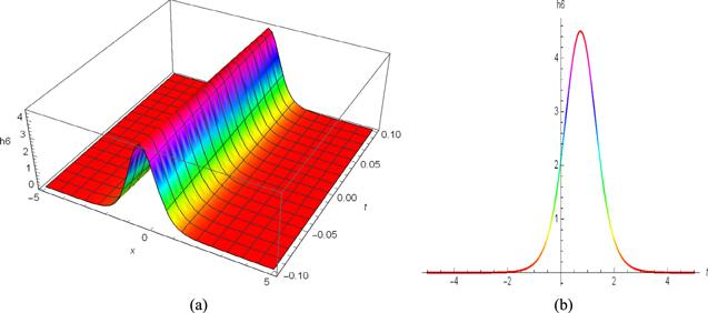
The solutions of equation (1.1 ) are as follows3.33 ) are shown in figures 9–11 by choosing arbitrary values of parameters.
$\begin{eqnarray}{h}_{6}(x,t)=\displaystyle \frac{{a}_{0}}{{c}_{0}+{c}_{1}\left(-\tfrac{1}{8}\,\tfrac{(4\,\sqrt{{b}_{2}}\,{e}^{\eta \sqrt{{b}_{2}}}\,{b}_{1}-4\,{b}_{2}\,{\left({e}^{\eta \sqrt{{b}_{2}}}\right)}^{2}+4\,{b}_{0}\,{b}_{2}-{b}_{1}^{2})}{{e}^{\eta \sqrt{{b}_{2}}}\,{b}_{2}^{\tfrac{3}{2}}}\right)},\end{eqnarray}$
where η = x −ϑt. The graphical illustrations in equation (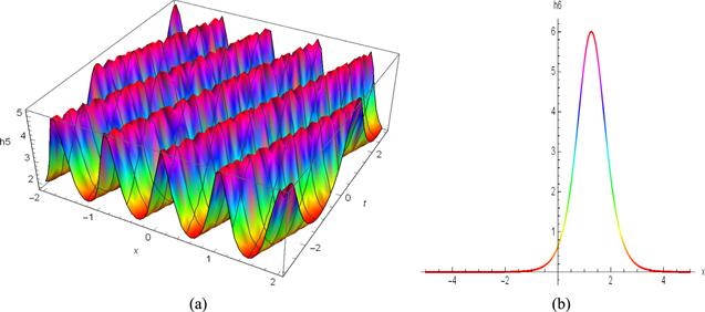
Figure 9. Dynamical behavior of equation ( |

Figure 10. Dynamical behavior of equation ( |
Figure 11. Dynamical behavior of equation ( |
4. Integrability via Painlevé test
In this section, the Painlevé test is applied to equation (1.1 ) for investigating the integrability of the proposed model.
First, find the dominant term by putting1.1 ) which gives c = −2. Now suppose
$\begin{eqnarray}h(x,t)=\lambda {\varrho }^{c}(x,t),\end{eqnarray}$
into equation ( $\begin{eqnarray}h(x,t)={h}_{0}(x,t){\varrho }^{c}(x,t).\end{eqnarray}$
By putting c = −2 in the above equation we get $\begin{eqnarray}h(x,t)={h}_{0}(x,t){\varrho }^{-2}(x,t),\end{eqnarray}$
Now comparing the coefficient of the lowest exponent of h(x, t) equal to zero, yields $\begin{eqnarray}{h}_{0}(x,t)=-\displaystyle \frac{6(s-\delta )}{m}{\left({\varrho }_{x}\right)}^{2},\end{eqnarray}$
where h0 is the initial integration constant.Following that, we compute the resonances associated with the dominating behavior by substituting1.1 ) and setting the coefficient of the lowest power of ϱ(x, t) to zero, we get4.8 ), we obtain4.9 ) into equation (1.1 ). The value of constants of integration k6, r = 1, 2, 3, 4, 5, 6 have been evaluated by putting the coefficients of smallest powers of ϱ(x, t) equal to zero. At level k = 1, we get1.1 ) is integrable.
$\begin{eqnarray}\begin{array}{l}h(x,t)=-\displaystyle \frac{6(s-\delta )}{m}{\left({\varrho }_{x}\right)}^{2}{\varrho }^{-2}(x,t)\\ \,+\,{h}_{k}(x,t){\varrho }^{-2+k}(x,t),\end{array}\end{eqnarray}$
by plugging the above into equation ( $\begin{eqnarray}{k}^{4}-14{k}^{3}+59{k}^{2}-46k-120=0.\end{eqnarray}$
Solving the above equation gives $\begin{eqnarray}k=-1,\,\,\,k=4,\,\,\,k=5,\,\,\,k=6.\end{eqnarray}$
Now we will look for integration constants to evaluate the compatibility constraints. Next, let us consider $\begin{eqnarray}h(x,t)={\varrho }^{c}(x,t)\,\displaystyle \sum _{k=0}^{{k}_{r}}\,{h}_{k}(x,t)\,{\varrho }^{k}(x,t).\end{eqnarray}$
Plugging the values c = −2 and kr = 6 into equation ( $\begin{eqnarray}h(x,t)={\varrho }^{-2}(x,t)\,\displaystyle \sum _{k=0}^{6}\,{h}_{k}(x,t)\,{\varrho }^{k}(x,t).\end{eqnarray}$
Putting equation ( $\begin{eqnarray}{h}_{1}(x,t)=\displaystyle \frac{6(s-\delta )}{m}\,{\varrho }_{{xx}}.\end{eqnarray}$
For k = 2, we obtain $\begin{eqnarray}\begin{array}{l}{h}_{2}(x,t)=\displaystyle \frac{1}{2\,m\,{\left({\varrho }_{x}\right)}^{2}}\,\left({\left({\varrho }_{x}\right)}^{2}({l}^{2}+\sigma )\right.\\ \left.+(s-\delta )\,\left(3\,{\left({\varrho }_{{xx}}\right)}^{2}-4\,{\varrho }_{x}\,{\varrho }_{{xxx}}\right)-{\left({\varrho }_{t}\right)}^{2}\right).\end{array}\end{eqnarray}$
For k = 3, we obtain $\begin{eqnarray}\begin{array}{l}{h}_{3}(x,t)=\displaystyle \frac{1}{2\,m\,{\left({\varrho }_{x}\right)}^{4}}\,\left(s-\delta )\,\left({\left({\varrho }_{x}\right)}^{2}\,{\varrho }_{{xxxx}}\right.\right.\\ \left.\left.+3\,{\left({\varrho }_{{xx}}\right)}^{2}-4\,{\varrho }_{x}\,{\varrho }_{{xx}}\,{\varrho }_{{xxx}}\right)+{\left({\varrho }_{x}\right)}^{2}\,{\varrho }_{{tt}}-{\varrho }_{{xx}}\,{\left({\varrho }_{t}\right)}^{2}\right).\end{array}\end{eqnarray}$
At level k = 4 , k = 5 and k = 6, we get $\begin{eqnarray}\begin{array}{l}{h}_{4}(x,t)={h}_{4}(x,t),\,\,\,{h}_{5}(x,t)={h}_{5}(x,t),\\ \,{h}_{6}(x,t)={h}_{6}(x,t).\end{array}\end{eqnarray}$
The compatibility constraints are met at the resonance levels k = 4, k = 5 and k = 6 proving that equation (5. Results discussion
In this article, we dive into the nonlinear Boussinesq water wave equation of the fourth order and see how it may be used to understand the movement of long waves in relatively shallow water. When waves enter regions of shallow water, they are influenced by the ocean floor. As a first goal, we solved the governing equation using a popular solution strategy known as the singular manifold method denoted by equation (3.14 ) and show the physical behavior of the solution in figures 1 and 2. Secondly, we solved the governing equation by using the unified method technique. We computed polynomial type solutions in the patterns of solitary waves denoted by equation (3.19 ), soliton waves denoted by equation (3.22 ), elliptic waves denoted by equation (3.26 ) and showed the physical behavior of the solution in figures 3–6 respectively. Similarly, we accumulated rational types of solutions in the fabrication of the periodic rational solutions equation (3.30 ) and the soliton rational solutions equation (3.33 ) and show the physical behavior of the solution in figures 7–11 respectively. The last motivation was to test the integrability of our governing PBE equation. We used the well-known P-test on our governing equation to complete our intended inquiry. According to the P-test technique to estimate the elementary constant of integration, which is provided in equation (4.4 ). We then estimated the resonances in equation (4.5 ). Finally, we evaluated the remaining integration constants indicated by equation (4.10 ) to equation (4.13 ). As a consequence, all of the P-test conditions for PBE are fulfilled and this equation successfully passes the P-test procedure and is therefore totally integrable.
6. Conclusion
In this study, we investigate the dynamics of shallow water waves using the Boussinesq equation with significant perturbation components. We derived scores of closed form soliton solutions to the perturbed Boussinesq equation in this work, including the bell-shaped soliton, kink-soliton, periodic-wave, singular-kink, and other forms of solitons associated with a variety of free parameters. These free parameters have significant ramifications, such as the ability to find cognizant answers in a unique fashion by setting alternative values of the free parameters from an individual solution. These soliton solutions have been derived for PBE, using the singular manifold method and unified technique. It is essential to note that nonlinear evaluation equation solutions are obtained using trigonometric, hyperbolic, rational, and exponential functions. This article provided soliton solutions for PBE, using the SMM technique and unified method. The SMM approach yields the single wave solution. We were successful in enumerating new types of PBE solutions as rational and polynomial using the UM technique. Similarly, we provided a recent integrability study of our governing model using the P-test, which demonstrated that the model is solvable by some integration technique. The 2D and 3D graphs predict the dynamical behavior of these solutions, which has been demonstrated to be very useful in the field of fluid dynamics for shallow water waves. The graphs are provided to demonstrate the right wave profiles. Some of the derived solutions are original, making them useful for the investigation of nonlinear physical processes. It may be claimed that the selected techniques are dependable, effective, and conformable and provide several compatible solutions to NLEEs encountered in mathematical physics, applied mathematics, and engineering.