Welcome to visit Communications in Theoretical Physics,
Mathematical Physics

A family of solutions of the time–space fractional longitudinal wave equation

  • Jian-Gen Liu , 1 ,
  • Yi-Ying Feng 2, 3
Expand
  • 1School of Mathematics and Statistics, Changshu Institute of Technology, Changshu 215500, Jiangsu, China
  • 2School of Mathematics and Statistics, Suzhou University, Suzhou 234000, Anhui, China
  • 3School of Mechanics and Civil Engineering, China University of Mining and Technology, Xuzhou 221116, Jiangsu, China

Received date: 2022-11-04

  Revised date: 2023-02-22

  Accepted date: 2023-05-29

  Online published: 2023-07-06

Copyright

© 2023 Institute of Theoretical Physics CAS, Chinese Physical Society and IOP Publishing

Abstract

In this article, we have studied a nonlinear time–space fractional longitudinal wave equation in the context of the conformable fractional derivative. Through the soliton ansatz method and a direct integration approach with the symmetry condition, new soliton and solitary wave solutions are derived. Furthermore, the existing conditions of these obtained solutions are also given in this text. These new results add to the existing literature. We believe that they can provide a new window into the understanding of this model.

Cite this article

Jian-Gen Liu , Yi-Ying Feng . A family of solutions of the time–space fractional longitudinal wave equation[J]. Communications in Theoretical Physics, 2023 , 75(7) : 075009 . DOI: 10.1088/1572-9494/acd998

1. Introduction

In recent years, the study of exact solutions in magneto-electro-elastic media (such as sensors, actuators and controllers) has attracted more and more attention from mathematicians and physicists [14]. As everyone knows, the governing equation that describes the propagation of solitons through magneto-electro-elastic media is modeled by a longitudinal wave equation of the form [1]
$\begin{eqnarray}\displaystyle \frac{{\partial }^{2}u}{\partial {t}^{2}}-{c}_{0}\displaystyle \frac{{\partial }^{2}u}{\partial {x}^{2}}-\displaystyle \frac{1}{2}{c}_{0}^{2}\displaystyle \frac{{\partial }^{2}{u}^{2}}{\partial {x}^{2}}-N\displaystyle \frac{{\partial }^{4}u}{\partial {t}^{2}{x}^{2}}=0,\end{eqnarray}$
where c0 is the linear longitudinal velocity of a magneto-electro-elastic circular rod and N > 0 is the dispersion parameter [1]. It is well known that equation (1) has been studied by many researchers, with solutions such as the one-soliton and peaked solitary wave solutions [2], the bright and singular soliton solutions [3], the hyperbolic function solitary wave solutions and plane wave solutions [4]. In addition, equation (1) can be reduced to the Boussinesq equation in the case of traveling wave solutions, which have N-soliton solutions [5]. Further, equation (1) can be viewed as a special case of the (2+1)-dimensional Boussinesq equation [6].
Fractional derivatives have the characteristics of heredity and memory. They are widely used in the fields of natural science and engineering technology. In general, nonlinear evolution equations of fractional order can better express scientific phenomena than differential equations of integer order. Therefore, we have mainly discussed the fractional version of equation (1) with the conformable fractional derivative in a magneto-electro-elastic circular rod. That is
$\begin{eqnarray}\begin{array}{l}\displaystyle \frac{{\partial }^{2\varepsilon }{\rm{\Phi }}(\chi ,\tau )}{\partial {\tau }^{2}}-{c}_{0}\displaystyle \frac{{\partial }^{2\varepsilon }{\rm{\Phi }}(\chi ,\tau )}{\partial {\chi }^{2}}-\displaystyle \frac{1}{2}{c}_{0}^{2}\displaystyle \frac{{\partial }^{2}{\rm{\Phi }}{\left(\chi ,\tau \right)}^{2}}{\partial {\chi }^{2}}\\ -N\displaystyle \frac{{\partial }^{4}{\rm{\Phi }}(\chi ,\tau )}{\partial {\tau }^{2}{\chi }^{2}}=0,\end{array}\end{eqnarray}$
where 0 < ϵ ≤ 1 is the fractional derivative order.
Here, we applied the soliton ansatz method and the direct integration approach to construct the soliton and solitary wave solutions of equation (2). The soliton and solitary wave solutions are interesting in soliton theory. They can be used to describe the velocity and amplitude of water wave propagation. The Hirota bilinear method and the Riemann–Hilbert method are systematic schemes to obtain the N-soliton solutions [7, 8]. Recently, the fractional Lie group method was used to solve fractional differential equations [9, 10] and the nonlocal group reduction was utilized to deal with nonlocal integrable equations [11, 12], attracting the attention of many scholars in the field of mathematical physics.
The plan of this article is as follows: in section 2, we give some basic definitions and theorems on the conformable fractional derivative. Through the soliton ansatz method, the soliton solutions of this considered model are obtained in section 3. In section 4, the solitary wave solutions are derived with the help of the direct integration approach. Meanwhile, their nonlinear dynamic behaviors are presented in two-dimensional graphics. In the last section, some important conclusions and discussions are shown.

2. Basic definitions

In the first place, some basic definitions and theorems on the conformable fractional derivative that will be used in the below text can be given.

[13, 14] Let $f:(0,\infty )\to R$, then the conformable fractional derivative of f of order α is defined as:

$\begin{eqnarray}{T}_{\alpha }(f)(t)=\mathop{\mathrm{lim}}\limits_{\delta \to 0}\displaystyle \frac{f(t+\delta {t}^{1-\alpha })-f(t)}{\delta },0\lt \alpha \leqslant 1,\end{eqnarray}$
for all $t\gt 0$.

[13] Let $\alpha \in (0,1]$ and $f,g$ be α-differentiable at a point t, then we have

1.

(1)${T}_{\alpha }({af}+{bg})={{aT}}_{\alpha }(f)+{{bT}}_{\alpha }(g),{\rm{for}}\,{\rm{all}}\,a,b\in R,$

2.

(2)${T}_{\alpha }({t}^{\lambda })=\lambda {t}^{\lambda -\alpha },{\rm{for}}\,{\rm{all}}\,\lambda \in R,$

3.

(3)${T}_{\alpha }({fg})={{fT}}_{\alpha }(g)+{{gT}}_{\alpha }(f),$

4.

(4)${T}_{\alpha }\left(\tfrac{f}{g}\right)=\tfrac{{{fT}}_{\alpha }(g)-{{gT}}_{\alpha }(f)}{{g}^{2}}.$

In addition, if f is differentiable, then ${T}_{\alpha }(f)(t)={t}^{1-\alpha }\tfrac{{\rm{d}}f}{{\rm{d}}t}$.

[14] Assume $f,g:[0,\infty )\to R$ are α-differentiable functions ($0\lt \alpha \leqslant 1$), then $f(g(t))$ is α-differentiable with $t\ne 0$ and $g(t)\ne 0$, we have

$\begin{eqnarray}{T}_{\alpha }(f\circ g)(t)=({T}_{\alpha }f)(g(t)){T}_{\alpha }(g)(t)g{\left(t\right)}^{\alpha -1}.\end{eqnarray}$
If t = 0, then we have
$\begin{eqnarray}{T}_{\alpha }(f\circ g)(0)=\mathop{\mathrm{lim}}\limits_{t\to {0}^{+}}({T}_{\alpha }f)(g(t)){T}_{\alpha }(g)(t)g{\left(t\right)}^{\alpha -1}.\end{eqnarray}$

[13, 14] Assume $a\geqslant 0$ and $t\geqslant a$. If f is a function defined on $(a,t]$ and $\alpha \in f$, then the α-fractional integral of f is defined by

$\begin{eqnarray*}{I}_{\alpha }^{a}(f)(t)={\int }_{a}^{t}\displaystyle \frac{f(x)}{{x}^{1-\alpha }}{dx}.\end{eqnarray*}$

[13, 14] Suppose $a\geqslant 0$ and $\alpha \in (0,1)$. Also, let f be a continuous function such that ${I}_{\alpha }^{a}(f)(t)$ exists. Then

$\begin{eqnarray*}{T}_{\alpha }{I}_{\alpha }^{a}(f)(t)=f(t).\end{eqnarray*}$

Note 1. Definition 1 coincides with the classical definitions of Riemann–Liouville and Caputo on polynomials [15, 16].
Note 2. When α → 1, the above definitions and theorems become the classical cases.
In what follows, we will use the conformable fractional derivative and theorems to solve the nonlinear time–space fractional longitudinal wave equation (2).

3. Soliton solutions of equation (2)

In order to get soliton solutions of equation (2), we first suppose that equation (2) has the form of solution as follows:
$\begin{eqnarray}\begin{array}{c}{\rm{\Pi }}(\xi )={\rm{\Phi }}(\chi ,\tau )=\alpha {{\rm{sech}} }^{p}(\xi ),\\ \xi =\frac{{\chi }^{\varepsilon }}{\varepsilon }-v\frac{{\tau }^{\varepsilon }}{\varepsilon },0\lt \varepsilon \leqslant 1,\end{array}\end{eqnarray}$
where α is the amplitude of the soliton, v is the velocity of the soliton and ϵ is the conformable fractional derivative.
Substituting (6) into (2) yields
$\begin{eqnarray}\begin{array}{l}{{\rm{sech}} }^{p}(\xi )\alpha \,{v}^{2}-{{\rm{sech}} }^{p}(\xi )\alpha \,{c}_{0}-\displaystyle \frac{1}{2}\,{{c}_{0}}^{2}{\alpha }^{2}{{\rm{sech}} }^{2p}(\xi )\\ -N{{\rm{sech}} }^{p}(\xi )(1-{{\rm{sech}} }^{2}(\xi ))\alpha \,{v}^{2}{p}^{2}\\ -N{{\rm{sech}} }^{p}(\xi )(1-{{\rm{sech}} }^{2}(\xi ))\alpha \,{c}^{2}p+N{{\rm{sech}} }^{p}(\xi )\alpha \,{v}^{2}p=0.\end{array}\end{eqnarray}$
Balancing the powers 2p and p + 2, gives
$\begin{eqnarray*}p=2.\end{eqnarray*}$
Substituting p = 2 into (6) and setting the coefficients of ${\rm{{\rm{sech}} }}{(\xi )}^{i},i\,=\,2,4$ to zero, one has that
$\begin{eqnarray}\left\{\begin{array}{l}-\displaystyle \frac{1}{2}\,{{c}_{0}}^{2}{\alpha }^{2}+6\,N\alpha \,{v}^{2}=0,\\ -4\,N\alpha \,{v}^{2}+\alpha \,{v}^{2}-\alpha \,{c}_{0}=0.\\ \end{array}\right.\end{eqnarray}$
Solving systems (8), we have
$\begin{eqnarray}\alpha =-\displaystyle \frac{212N}{{c}_{0}\left(4\,N-1\right)},\,v=\pm \sqrt{-\displaystyle \frac{{c}_{0}}{4\,N-1}},\end{eqnarray}$
where the existing conditions of soliton solutions are
$\begin{eqnarray}\displaystyle \frac{{c}_{0}}{4\,N-1}\leqslant 0\,\,{\rm{and}}\,\,N\ne \displaystyle \frac{1}{4}.\end{eqnarray}$
Therefore, we can obtain two soliton solutions of equation (2) with (6) as follows:
$\begin{eqnarray}\begin{array}{rcl}{\rm{\Phi }}(\chi ,\tau ) & = & -\displaystyle \frac{12N}{{c}_{0}\left(4\,N-1\right)}\\ & & \times \,{{\rm{sech}} }^{2}\left(-\displaystyle \frac{{\chi }^{\varepsilon }}{\varepsilon }\pm \displaystyle \frac{{\tau }^{\varepsilon }}{\varepsilon }\sqrt{-\displaystyle \frac{{c}_{0}}{4\,N-1}}\right).\end{array}\end{eqnarray}$
Similarly, if the following form of ansatz solution of equation (2) holds
$\begin{eqnarray}\begin{array}{rcl}{\rm{\Pi }}(\xi ) & = & {\rm{\Phi }}(\chi ,\tau )=\alpha \csc {{\rm{h}}}^{p}(\xi ),\\ \xi & = & \displaystyle \frac{{\chi }^{\varepsilon }}{\varepsilon }-v\displaystyle \frac{{\tau }^{\varepsilon }}{\varepsilon },0\lt \varepsilon \leqslant 1,\end{array}\end{eqnarray}$
then we can obtain the other two soliton solutions of the forms
$\begin{eqnarray}\begin{array}{rcl}{\rm{\Phi }}(\chi ,\tau ) & = & \displaystyle \frac{12N}{{c}_{0}\left(4\,N-1\right)}\\ & & \times \,{\mathrm{csch}}^{2}\left(-\displaystyle \frac{{\chi }^{\varepsilon }}{\varepsilon }\pm \displaystyle \frac{{\tau }^{\varepsilon }}{\varepsilon }\sqrt{-\displaystyle \frac{{c}_{0}}{4\,N-1}}\right).\end{array}\end{eqnarray}$
In order to see the nonlinear evolution processes of solutions (11) and (13) more directly, we show their three-dimensional and two-dimensional diagrams in figure 1.
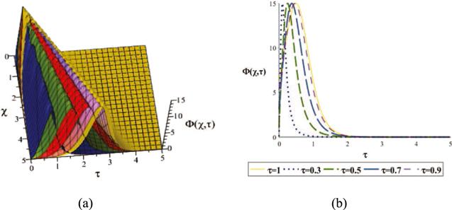
Figure 1. (a) Soliton solution (11) with parameters c0 = 0.8, N = 0.2, ϵ = 0.3/0.5/0.7/0.9/1 (from left to right). (b) Two-dimensional plot, corresponding to the first graph.
From figure 1, we can see that the fractional order ϵ did not change the amplitude of the soliton waves, but slightly changes their widths.

4. Solitary wave solutions of equation (2)

In this section, we discuss the solitary wave solutions of equation (2) with the symmetry condition. A wave transformation presents that
$\begin{eqnarray}{\rm{\Pi }}(\xi )={\rm{\Phi }}(\chi ,\tau ),\xi =\displaystyle \frac{{\chi }^{\varepsilon }}{\varepsilon }-c\displaystyle \frac{{\tau }^{\varepsilon }}{\varepsilon },0\lt \varepsilon \leqslant 1,\end{eqnarray}$
where c is the velocity of the solitary wave.
Substituting (14) into (2) yields
$\begin{eqnarray}{c}^{2}{\rm{\Pi }}^{\prime\prime} -{c}_{0}{\rm{\Pi }}^{\prime\prime} -\displaystyle \frac{1}{2}{c}_{0}^{2}({{\rm{\Pi }}}^{2})^{\prime\prime} -{cN}{{\rm{\Pi }}}^{\unicode{x02057}}=0.\end{eqnarray}$
We can see that there exists the symmetry condition
$\begin{eqnarray}{\rm{\Pi }}(\xi )={\rm{\Pi }}(-\xi ),\xi \in (-\infty ,+\infty ).\end{eqnarray}$
Hence, we only need to consider the solutions in the interval ξ ≥ 0.
Integrating equation (15) twice, and taking the integration constants to be equal to zero, one obtains
$\begin{eqnarray}({c}^{2}+{c}_{0}){\rm{\Pi }}-\displaystyle \frac{1}{2}{c}_{0}^{2}{{\rm{\Pi }}}^{2}-{c}^{2}N{\rm{\Pi }}^{\prime\prime} =0,\xi \geqslant 0.\end{eqnarray}$
Separating variables and integrating once more, equation (17) leads to
$\begin{eqnarray}\pm \xi =\int \displaystyle \frac{{\rm{d}}{\rm{\Pi }}}{{\rm{\Pi }}\sqrt{\tfrac{{c}^{2}-{c}_{0}}{{c}^{2}N}-\tfrac{{c}_{0}^{2}}{3{c}^{2}N}{\rm{\Pi }}}},\xi \geqslant 0.\end{eqnarray}$
This implies the existing condition of solution
$\begin{eqnarray}{\rm{\Pi }}\leqslant \displaystyle \frac{3{c}^{2}-3{c}_{0}}{{c}_{0}^{2}}.\end{eqnarray}$
Hence, we suppose c2 > c0.
From equation (18), two kinds of solitary wave solutions can be obtained in the following:
Case 1:
When $0\leqslant {\rm{\Pi }}\leqslant \tfrac{3{c}^{2}-3{c}_{0}}{{c}_{0}^{2}}$, we have a solitary wave solution for equation (18)
$\begin{eqnarray}\begin{array}{c}{\rm{\Pi }}(\xi )=\frac{3({c}^{2}-{c}_{0})}{{c}_{0}^{2}}{{\rm{sech}} }^{2}\left\{\frac{1}{2}\sqrt{\frac{{c}^{2}-{c}_{0}}{{c}^{2}N}}\xi +\lambda \right\},\\ \xi \geqslant 0,\lambda \geqslant 0.\end{array}\end{eqnarray}$
Therefore, we have the solitary solution for equation (18) with symmetry condition (16) as follows:
$\begin{eqnarray}\begin{array}{c}{\rm{\Pi }}(\xi )=\frac{3({c}^{2}-{c}_{0})}{{c}_{0}^{2}}{{\rm{sech}} }^{2}\left\{\frac{1}{2}\sqrt{\frac{{c}^{2}-{c}_{0}}{{c}^{2}N}}\left|\xi \right|+\lambda \right\},\\ \xi \in (-\infty ,+\infty ),\lambda \geqslant 0,\end{array}\end{eqnarray}$
in the whole interval.
So, we have the following solitary wave solution
$\begin{eqnarray}\begin{array}{ccl}{\rm{\Phi }}(\chi ,\tau ) & = & \frac{3({c}^{2}-{c}_{0})}{{c}_{0}^{2}}{{\rm{sech}} }^{2}\\ & & \times \,\left\{\frac{1}{2}\sqrt{\frac{{c}^{2}-{c}_{0}}{{c}^{2}N}}\left|\frac{{\chi }^{\varepsilon }}{\varepsilon }-c\frac{{\tau }^{\varepsilon }}{\varepsilon }\right|+\lambda \right\},\lambda \geqslant 0.\end{array}\end{eqnarray}$
Case 2:
When ${\rm{\Pi }}\leqslant 0\leqslant \tfrac{3{c}^{2}-3{c}_{0}}{{c}_{0}^{2}}$, we can get the other solitary wave solution for equation (18)
$\begin{eqnarray}\begin{array}{c}{\rm{\Pi }}(\xi )=-\frac{3({c}^{2}-{c}_{0})}{{c}_{0}^{2}}{\mathrm{csch}}^{2}\left\{\frac{1}{2}\sqrt{\frac{{c}^{2}-{c}_{0}}{{c}^{2}N}}\xi +\delta \right\},\\ \xi \geqslant 0,\delta \gt 0.\end{array}\end{eqnarray}$
Therefore, we have the solitary solution for equation (18) with symmetry condition (16) as follows:
$\begin{eqnarray}\begin{array}{c}{\rm{\Pi }}(\xi )=-\frac{3({c}^{2}-{c}_{0})}{{c}_{0}^{2}}{\mathrm{csch}}^{2}\left\{\frac{1}{2}\sqrt{\frac{{c}^{2}-{c}_{0}}{{c}^{2}N}}\left|\xi \right|+\delta \right\},\\ \xi \in (-\infty ,+\infty ),\delta \gt 0,\end{array}\end{eqnarray}$
in the whole interval.
So, we have the following solitary wave solution
$\begin{eqnarray}\begin{array}{c}{\rm{\Phi }}(\chi ,\tau )=-\frac{3({c}^{2}-{c}_{0})}{{c}_{0}^{2}}{\mathrm{csch}}^{2}\\ \times \,\left\{\frac{1}{2}\sqrt{\frac{{c}^{2}-{c}_{0}}{{c}^{2}N}}\left|\frac{{\chi }^{\varepsilon }}{\varepsilon }-c\frac{{\tau }^{\varepsilon }}{\varepsilon }\right|+\delta \right\},\delta \gt 0.\end{array}\end{eqnarray}$
We plotted the nonlinear evolution behaviors with different parameters of solitary wave solution (22) by figure 2.
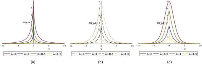
Figure 2. Solitary wave solution (22) with parameters c = 1, c0 = 0.5, N = 0.5, χ = 0. (a) ϵ = 0.4 (b) ϵ = 0.7. (c) ϵ = 1.
From figure 2, we can see that the fractional order ϵ did not change the amplitude of the solitary waves. Besides, when λ = 0, solution (22) is a solitary wave solution, while solution (22) is a solitary peak wave solution if λ > 0. That is to say, it is not differentiable at the peak of the solitary wave solution.

5. Conclusions and discussion

By applying two different schemes, we derived some new soliton solutions and solitary wave solutions to the nonlinear time–space fractional longitudinal wave equation. After analyzing them, we found that these results became the classical cases of ϵ → 1. In addition, the fractional order ϵ did not change the amplitude of the soliton solutions and solitary wave solutions from figures 1 and 2. In the future, we will further study the rational solutions and integrability of this considered model.

This work is supported by the Yue-Qi Scholar of the China University of Mining and Technology (No.102504180004).

1
Xue C X Pan E Zhang S Y 2011 Solitary waves in a magneto-electro-elastic circular rod Smart Mater. Struct. 20 105010

DOI

2
Yang S Xu T 2016 1-soliton and peaked solitary wave solutions of nonlinear longitudinal wave equation in magneto-electro-elastic circular rod Nonlinear Dyn. 87 2735 2739

3
Younis M Ali S 2015 Bright, dark, and singular solitons in magneto-electro-elastic circular rod Waves Random Complex Media 25 549 555

DOI

4
Zhou Q 2016 Analytical study of solitons in magneto-electro-elastic circular rod Nonlinear Dyn. 83 1403 1408

DOI

5
Ma W-X Li C-X He J 2009 A second Wronskian formulation of the Boussinesq equation Nonlinear Anal. Theory Methods Appl. 70 4245 4258

DOI

6
Yu Z Zhang Z Yang H 2021 (2+1)-dimensional coupled Boussinesq equations for Rossby waves in two-layer cylindrical fluid Commun. Theor. Phys. 73 115005

DOI

7
Ma W-X 2022 Soliton solutions by means of Hirota bilinear forms Partial Differ. Equ. Appl. Math. 5 100220

DOI

8
Ma W-X 2021 Nonlocal PT-symmetric integrable equations and related Riemann–Hilbert problems Partial Differ. Equ. Appl. Math. 4 100190

DOI

9
Liu J-G 2021 Group analysis of the time fractional (3+1)-dimensional KdV-type equation Fractals 29 2150169

10
Liu J-G 2022 On fractional symmetry group scheme to the higher dimensional space and time fractional dissipative Burgers equation Int. J. Geom. Methods Mod. Phys. 19 2250173

11
Ma W-X 2022 Integrable nonlocal nonlinear Schrödinger equations associated with so(3, ) Proc. Am. Math. Soc. B 9 1 11

DOI

12
Ma W-X 2022 Reduced non-local integrable NLS hierarchies by pairs of local and non-local constraints Int. J. Appl. Comput. Math. 8 206

13
Khalil R Horani M A Yousef A 2014 A new definition of fractional derivative J. Comput. Appl. Math. 264 65 70

DOI

14
Abdeljawad T 2014 On conformable fractional calculus J. Comput. Appl. Math. 279 57 66

15
Samko S Kilbas A A Marichev O 1993 Fractional Integrals and Derivatives: Theory and Applications Yverdon, Switzerland Gordon and Breach

16
Yang X J 2019 General Fractional Derivatives: Theory, Methods and Applications New York CRC Press

Outlines

/