


1. Introduction
Recently, some nonautonomous soliton solutions of the Gross–Pitaevskii (GP) equation with linear and harmonic oscillator potentials are presented, which can generalize some novel phenomena in the plethora [1]. A few of the stable bright and dark solitons of the GP equation with varying dispersion and gain (or absorption) are considered in [2]. The peculiar nonlinear wave phenomena (the parallel waves) are presented in optics and Bose condensates, which can generalize the nonautonomous optical and matter-wave solitons in the GP equation [3]. Some exact nonautonomous matter-wave solutions (W-bright soliton, U-shaped dark soliton, periodic wave soliton, and rational soliton) are derived in [4]. Some nonautonomous discrete rogue waves are reported in discrete soliton equations [5–8], and some nonautonomous discrete bright soliton solutions are considered in the generalized GP equation [9]. Especially, some GP equations with parity-time(PT)-symmetric potentials are studied via the inverse scattering transformation, then many physically relevant soliton solutions are obtained in [10–14]. Some important solutions of the nonlinear Schrödinger equation (NLS) are presented, the multi-solitons, n-periodic solutions and some mixed solutions are obtained via Darboux transformation in [15]. Soliton, breather and rogue wave solutions of the NLS are considered by using a deep learning method in [16]. The breathers and rogue waves on the double-periodic background are successfully constructed by using a plane wave seed solution in [17].
The fractional order integrals and derivatives have been presented by Leibniz, Liouville, Riemann, Grunwald and Letnikov [18, 19], which have some important applications, such as the kinetic theories [20, 21], the statistical mechanics [22, 23] and some dynamics of complex media. Some applications and vector calculus of non-integer dimensional space are presented in fractal media [24]. A fractional integral and its physical interpretation are considered in [25], in which some equations in fractional derivatives can describe the evolution of physical systems. A new application of a fractal concept to quantum physics is developed in [26]. There are a number of research areas in physics that employ fractional calculus in [27]. Some of the fractional-order models are more appropriate in many real materials.
Laskin presented the fractional nonlinear Schrödinger (FNLS) equation in [28, 29], and the FNLS equation was introduced into optics in 2015 [30]. A chirped Gaussian beam propagation of linear cases is investigated in the FNLS equation [31]. Reference [32] gives some localization delocalization transition points and some anti-Anderson localization of the quasi-periodic lattices in the FNLS equation. The FNLS equation with harmonic oscillator potentials is considered in [33], and the FNLS equation with or without a potential is presented in [34]. Some solitons of the FNLS equation are derived, which can tune the nonlinear effects [35], and some height-dimensional solitons of an FNLS equation are also obtained in [36]. Recently, some novel gap solitons of a FNLS equation are investigated in [37]. Some novel wave perturbation properties of nonlinear (3+1)-dimensional Vakhnenko-Parkes equation are considered by using the sine-Gordon expansion method in [38]. A newly developed method of rational sine-Gordon expansion method is presented to find novel exact solutions of nonlinear differential equations in [39]. In this paper, we further extend the sine-Gordon method to the fractional soliton solution of a space-time fractional Gross–Pitaevskii (FGP) equation, which has some novel dynamic behaviors.
How to obtain the fractional soliton solution of a space-time FGP equation is important work. We further extend and investigate the non-autonomous bright–dark soliton (NBDS) solutions and some novel dynamic behaviors of the conformable space-time FGP equation with an external potential, which is different from those results in the previous works. We consider the relations between the space-time FGP equation and the FNLS equation with group velocity dispersion coefficient and spatiotemporal dispersion and analyze the properties of the obtained equation. Furthermore, we consider the effect of the parameters α, β in nonautonomous bright–dark solutions of the space-time FGP equation. We present a method to control the wave prolongs via the fractional spatial–temporal part of α, β. Some novel dynamics are obtained via the different parameters, including bright soliton solution, novel “h”-shape dark soliton solution and some interactions of the NBDSs. We also consider several controlling methods for nonautonomous fractional bright–dark soliton solutions, including spatial management and temporal–spatial management. We can derive a method to conformable the temporal–spatial FGP equation.
In section 2 , we consider some information of fractional differential forms. In section 3 , we describe the similarity transformation of the space-time FGP equation. In section 4 , some exact fractional nonautonomous bright–dark soliton solutions and their interactions with temporal-spatial management are investigated analytically. Finally, some conclusions are given.
2. Some fractional derivatives
The derivatives of arbitrary real order p can be considered as an interpolation of this sequence of operators. We will use for it the notion suggested and used by Davis [17], namely
$\begin{eqnarray}{}_{a}{{\boldsymbol{D}}}_{t}^{p}f(t),\end{eqnarray}$
the short name for derivatives of arbitrary order is fractional derivatives. The subscripts a and t denote the two limits related to the operation of fractional differentiation.Following Ross [18], we will call them the terminals of fractional differentiation. The appearance of the terminals in the symbol of fractional is essential. This helps to avoid ambiguities in the applications of fractional derivatives to real problems. The integral of arbitrary p > 0 order is given2 ) satisfies the asymptotic condition of ${}_{a}{{\boldsymbol{D}}}_{t}^{-p}f(T)$ at T = 0.
$\begin{eqnarray}\begin{array}{rcl}{}_{a}{{\boldsymbol{D}}}_{t}^{-p}f(t) & = & \displaystyle \sum _{k=0}^{m}\displaystyle \frac{{f}^{(k)}(a){\left(t-a\right)}^{p+k}}{{\rm{\Gamma }}(p+k+1)}+\displaystyle \frac{1}{{\rm{\Gamma }}(p+k+1)}\\ & & \times \,{\int }_{a}^{t}{\left(t-\tau \right)}^{p+m}{f}^{(m+1)}(\tau ){\rm{d}}\tau ,\end{array}\end{eqnarray}$
and equation (A fractional derivative
$\begin{eqnarray*}{}_{b}{{\boldsymbol{D}}}_{T}^{q}g(T)=\mathop{\mathrm{lim}}\limits_{r\to +-\infty ,{sr}\to T-b}{g}_{s}^{(q)}(T)\end{eqnarray*}$
$\begin{eqnarray}\begin{array}{l}=\displaystyle \sum _{v=0}^{l}\displaystyle \frac{{g}^{(k)}(b){\left(T-b\right)}^{-q+v}}{{\rm{\Gamma }}(-q+v+1)}+\displaystyle \frac{1}{{\rm{\Gamma }}(-q+v+1)}\\ \quad \times {\int }_{b}^{T}{\left(T-\tau \right)}^{l-q}{g}^{(l+1)}(\tau ){\rm{d}}\tau ,\end{array}\end{eqnarray}$
here the derivative g(v)(T) is a consecutive function with (v = 1, 2,…,l + 1) in [b, T], the l satisfies l > q + 1.In order to easy to apply the fractional calculus, the Riemann-Liouville definition is introduced with p(n ≤ p ≤ n + 1)
$\begin{eqnarray}{}_{a}{{\boldsymbol{D}}}_{t}^{p}f(T)={\left(\displaystyle \frac{{\rm{d}}}{{\rm{d}}{T}}\right)}^{n+1}{\int }_{a}^{T}{\left(T-\tau \right)}^{n-p}f(\tau ){\rm{d}}\tau .\end{eqnarray}$
Based on the Riemann-Liouville definition (4 ), we can derive that the f(t) is the r-order (r < 1) integrable function at τ = a, when the f(τ) is a continuous integrable function in (a,t),
$\begin{eqnarray*}\mathop{\mathrm{lim}}\limits_{\tau \to a}{\left(\tau -a\right)}^{r}f(t)=C,\end{eqnarray*}$
and the ${f}^{-1}(T)={\int }_{a}^{t}\,f(\tau )\,{\rm{d}}\tau $ is 0 with t → a.We get a general equation
$\begin{eqnarray}{g}^{-s}(T)=\displaystyle \frac{1}{{\rm{\Gamma }}(s)}{\int }_{b}^{T}{\left(T-w\right)}^{s-1}g(w){\rm{d}}{w}.\end{eqnarray}$
Then, we derive the following formulas under the conditions n ≥ 1 and k ≥ 0, $\begin{eqnarray*}{g}^{-k-n}(t)=\displaystyle \frac{1}{{\rm{\Gamma }}(n)}{{\boldsymbol{D}}}^{-k}{\int }_{a}^{k}{\left(t-\tau \right)}^{n-1}g(\tau ){\rm{d}}\tau ,\end{eqnarray*}$
$\begin{eqnarray*}{g}^{k-n}(t)=\displaystyle \frac{1}{{\rm{\Gamma }}(n)}{{\boldsymbol{D}}}^{k}{\int }_{a}^{k}{\left(t-\tau \right)}^{n-1}g(\tau ){\rm{d}}\tau ,\end{eqnarray*}$
here D−k(k ≥ 0) and Dk(k ≥ 0) represent the k interacted-differentiation.If replacing an integer n by a real p > 0, the Cauchy formula (5 ) can be written as5 ), and p is weak for p > 0.
$\begin{eqnarray}{}_{a}{{\boldsymbol{D}}}_{t}^{-p}g(t)=\displaystyle \frac{1}{{\rm{\Gamma }}(p)}\,{\int }_{a}^{t}{\left(t-\tau \right)}^{p-1}\,g(\tau )\,{\rm{d}}\tau ,\end{eqnarray}$
and n satisfies n ≥ 1 in equation (We consider the assumption6 ), the arbitrary order integration is obtained, when the f(t) is a continuous function with t ≥ a
$\begin{eqnarray}\mathop{\mathrm{lim}}\limits_{p\to 0}{\,}_{a}{{\boldsymbol{D}}}_{t}^{-p}f(t)=f(t),\end{eqnarray}$
and can get ${}_{a}{{\boldsymbol{D}}}_{t}^{0}f(t)=f(t)$. Based on the formula ( $\begin{eqnarray}{}_{a}{{\boldsymbol{D}}}_{t}^{-p}{(}_{a}{{\boldsymbol{D}}}_{t}^{-q})f(t){=}_{a}{{\boldsymbol{D}}}_{t}^{-p-q}f(t).\end{eqnarray}$
Indeed, we have $\begin{eqnarray*}{}_{b}{{\boldsymbol{D}}}_{T}^{-q}{(}_{b}{{\boldsymbol{D}}}_{T}^{-j})g(T)=\displaystyle \frac{1}{{\rm{\Gamma }}(j)}{\int }_{b}^{T}{\left(T-w\right)}^{j-1}{\,}_{b}{{\boldsymbol{D}}}_{T}^{-q}g(w){\rm{d}}{w}\end{eqnarray*}$
$\begin{eqnarray*}=\displaystyle \frac{1}{{\rm{\Gamma }}(q){\rm{\Gamma }}(j)}{\int }_{b}^{T}{\left(T-w\right)}^{j-1}{dw}{\int }_{b}^{T}{\left(T-\xi \right)}^{q-1}g(\xi ){\rm{d}}\xi \end{eqnarray*}$
$\begin{eqnarray*}=\displaystyle \frac{1}{{\rm{\Gamma }}(q){\rm{\Gamma }}(j)}{\int }_{b}^{T}g(\xi )d\xi {\int }_{b}^{T}{\left(T-w\right)}^{j-1}{\left(T-\xi \right)}^{q-1}{\rm{d}}{w}\end{eqnarray*}$
$\begin{eqnarray*}=\displaystyle \frac{1}{{\rm{\Gamma }}(q+j)}{\int }_{b}^{T}{\left(T-z\right)}^{q+j-1}g(z){\rm{d}}{z}\end{eqnarray*}$
$\begin{eqnarray*}{=}_{b}\,{{\boldsymbol{D}}}_{T}^{-q-j}g(T).\end{eqnarray*}$
If we consider the parameters of q and j, we can obtain $\begin{eqnarray}{}_{b}{{\boldsymbol{D}}}_{T}^{-q}{(}_{b}{{\boldsymbol{D}}}_{T}^{-j})g(T){=}_{b}{{\boldsymbol{D}}}_{T}^{-j}{(}_{b}{{\boldsymbol{D}}}_{T}^{-q})g(T){=}_{b}{{\boldsymbol{D}}}_{T}^{-q-j}g(T).\end{eqnarray}$
Next, we give some properties of the fractional Riemann–Liouville (RL) derivative with q > 0 and T > b10 ) are the left-form fractional inverse operators of q.
$\begin{eqnarray*}{}_{b}{{\boldsymbol{D}}}_{T}^{q}{(}_{b}{{\boldsymbol{D}}}_{T}^{-q}g(T))=g(T),\end{eqnarray*}$
$\begin{eqnarray*}{}_{b}{{\boldsymbol{D}}}_{T}^{-q}{(}_{b}{{\bf{D}}}_{T}^{q}g(T))\ne g(T),\end{eqnarray*}$
$\begin{eqnarray}{}_{b}{{\boldsymbol{D}}}_{T}^{s}{(}_{b}{{\boldsymbol{D}}}_{T}^{q}g(T))={}_{b}{{\boldsymbol{D}}}_{T}^{s+q}g(T),\end{eqnarray}$
where the fractional RL operators (A product rule is given rise to as following
$\begin{eqnarray}{{\boldsymbol{D}}}_{t}^{p}(f(t)g(t))=\displaystyle \sum _{j=0}^{\infty }\left(\begin{array}{c}p\\ j\end{array}\right){{\boldsymbol{D}}}_{t}^{p-j}f(t){{\boldsymbol{D}}}_{t}^{j}g(t).\end{eqnarray}$
The improved fractional RL derivative is considered, which has the form in the definition [40]
$\begin{eqnarray}\begin{array}{l}{{\boldsymbol{D}}}_{x}^{\alpha }f(x)\\ =\left\{\begin{array}{l}\displaystyle \frac{1}{{\rm{\Gamma }}(1-\alpha )}{\int }_{0}^{x}{\left(x-\phi \right)}^{-\alpha -1}[f(\phi )-f(0)]d\phi \,\,\,\alpha \lt 0,\\ \displaystyle \frac{1}{{\rm{\Gamma }}(-\alpha )}\displaystyle \frac{d}{{dx}}{\int }_{0}^{x}{\left(x-\phi \right)}^{-\alpha }[f(\phi )-f(0)]d\phi \,\,\,0\lt \alpha \lt 1,\\ {\left[{F}^{(\alpha -a)(x)}\right]}^{(a)}\qquad a\lt \alpha \lt a+1,a\gt 1,\end{array}\right.\end{array}\end{eqnarray}$
and the related properties in [41, 42] $\begin{eqnarray}\left\{\begin{array}{l}{{\boldsymbol{D}}}_{x}^{\alpha }{x}^{k}=\displaystyle \frac{{\rm{\Gamma }}(k+1)}{{\rm{\Gamma }}(k+1-\alpha )}{x}^{k-\alpha },k\gt 0,\\ {{\boldsymbol{D}}}_{x}^{\alpha }({ce}(x))=c({{\boldsymbol{D}}}_{x}^{\alpha }e(x)),\\ {{\boldsymbol{D}}}_{x}^{\alpha }(b(x)e(x))={\delta }_{x}[b(x)({{\boldsymbol{D}}}_{x}^{\alpha }e(x))+e(x)({{\boldsymbol{D}}}_{x}^{\alpha }b(x))],\\ {{\boldsymbol{D}}}_{x}^{\alpha }[a(\theta (x)]={\delta }_{x}{a}_{\theta }^{{\prime} }{{\boldsymbol{D}}}_{x}^{\alpha }\theta (x)\,{or}\,{D}_{x}^{\alpha }[a(\theta (x)]={\delta }_{x}{{\boldsymbol{D}}}_{x}^{\alpha }a(\theta ){\left({\theta }_{x}^{{\prime} }\right)}^{\alpha },\end{array}\right.\end{eqnarray}$
with the fractal index δx determined using a gamma function, the value δx is equal to one [43].3. Similarity reduction for the space-time FGP equation
The space-time FGP equation can describe the pulse propagation in the picosecond or femtosecond regime of the birefringent optical fibers, which has the following form:14 ) becomes the original NLS equation with group velocity dispersion coefficient and second-order spatiotemporal dispersion coefficients.
$\begin{eqnarray}\begin{array}{l}{\rm{i}}(\delta {{\boldsymbol{D}}}_{t}^{\alpha }{\rm{\Psi }}+{{\boldsymbol{D}}}_{x}^{\beta }{\rm{\Psi }})+\alpha (t){{\boldsymbol{D}}}_{t}^{2\alpha }{\rm{\Psi }}+\beta (t){{\boldsymbol{D}}}_{x}^{2\beta }{\rm{\Psi }}\\ \quad +g(t)| {\rm{\Psi }}{| }^{2}{\rm{\Psi }}+v(x,t){\rm{\Psi }}+{\rm{i}}\gamma (t){\rm{\Psi }}=0,\end{array}\end{eqnarray}$
here the ψ = ψ(x, t) denotes a electromagnetic component field, v(x, t) is a trapping potential, the x and t represent the distance propagation and local time respectively, β(t) is the group velocity dispersion, g(t) can describe nonlinearity, α(t) is the self-steepening, and the γ(t) of time is the gain/loss coefficient. When α = 1, equation (A similar transformation of the fractional NLS equation is considered, and some soliton solutions of the space-time fractional NLS equation are derived in [44]
$\begin{eqnarray}i(\delta {{\boldsymbol{D}}}_{T}^{\alpha }{\rm{\Phi }}+{{\boldsymbol{D}}}_{X}^{\beta }{\rm{\Phi }})+\upsilon {{\boldsymbol{D}}}_{T}^{2\alpha }{\rm{\Phi }}+\gamma {{\boldsymbol{D}}}_{X}^{2\beta }{\rm{\Phi }}+| {\rm{\Phi }}{| }^{2}{\rm{\Phi }}=0,\end{eqnarray}$
here Φ is a function of X and T, the δ describes a ratio of group speed, &ugr; is a coefficient of the group velocity dispersion, and γ is a coefficient of the spatial dispersion.Taking the ansatz method, the solution of the physical field ψ(x, t) is presented14 ) and (15 ) can be constructed relations via the ansatz (16 ). Substituting the ansatz (16 ) into equation (14 ), the systems are obtained as follows:
$\begin{eqnarray}{\rm{\Psi }}(x,t)=\rho (t){{\rm{e}}}^{{\rm{i}}\varphi (x,t)}{\rm{\Phi }}(X(x,t),T(t)),\end{eqnarray}$
where φ(x, t) and ρ(t) satisfy indicated variables. Equations ( $\begin{eqnarray}\left\{\begin{array}{l}{\rm{i}}{{\rm{e}}}^{{\rm{i}}\varphi (x,t)}{\rm{\Phi }}:\delta {{\boldsymbol{D}}}_{t}^{\alpha }\rho (t)+2\alpha (t){{\boldsymbol{D}}}_{t}^{\alpha }\rho {{\boldsymbol{D}}}_{t}^{\alpha }\varphi (x,t)+\gamma (t)\rho ,\\ {{\rm{e}}}^{{\rm{i}}\varphi (x,t)}{\rm{\Phi }}:\rho {{\boldsymbol{D}}}_{t}^{\alpha }\phi +\rho {{\boldsymbol{D}}}_{x}^{\beta }\phi +\alpha (t)({{\boldsymbol{D}}}_{t}^{2\alpha }\rho -\rho \alpha (t)({{\boldsymbol{D}}}_{t}^{2\alpha }\phi )+\beta (t){{\boldsymbol{D}}}_{x}^{2\beta }\phi +v(x,t)\rho ,\\ {\rm{i}}{{\rm{e}}}^{{\rm{i}}\varphi (x,t)}{{\boldsymbol{D}}}_{X}^{\alpha }{\rm{\Phi }}:\delta \rho {{\boldsymbol{D}}}_{t}^{\alpha }X+2\alpha (t)\rho {{\boldsymbol{D}}}_{t}^{\alpha }\varphi (x,t){{\boldsymbol{D}}}_{t}^{\alpha }X,\\ {{\rm{e}}}^{{\rm{i}}\varphi (x,t)}{{\boldsymbol{D}}}_{X}^{\alpha }{\rm{\Phi }}:2\alpha (t){{\boldsymbol{D}}}_{t}^{\alpha }\rho {{\boldsymbol{D}}}_{t}^{\alpha }X+\rho \alpha (t){{\boldsymbol{D}}}_{t}^{2\alpha }X,\\ {{\rm{e}}}^{{\rm{i}}\varphi (x,t)}{{\boldsymbol{D}}}_{T}^{\alpha }{\rm{\Phi }}:2\alpha (t){{\boldsymbol{D}}}_{t}^{\alpha }\rho {{\boldsymbol{D}}}_{t}^{\alpha }T+\rho \alpha (t){{\boldsymbol{D}}}_{t}^{2\alpha }T,\\ {{\rm{e}}}^{{\rm{i}}\varphi (x,t)}{{\boldsymbol{D}}}_{X}^{\beta }{\rm{\Phi }}:\rho {{\boldsymbol{D}}}_{x}^{2\beta }X,\\ {v}^{{\rm{i}}\varphi (x,t)}{{\boldsymbol{D}}}_{X}^{2\beta }{\rm{\Phi }}:\alpha (t){\left({v}_{t}^{\alpha }X\right)}^{2},\\ \displaystyle \frac{\delta {{\boldsymbol{D}}}_{t}^{\alpha }T+2\alpha (t){{\boldsymbol{D}}}_{t}^{\alpha }\rho {{\boldsymbol{D}}}_{t}^{\alpha }T}{\delta }=\displaystyle \frac{{{\boldsymbol{D}}}_{x}^{\beta }X+2\beta (t){{\boldsymbol{D}}}_{t}^{\beta }\rho {{\boldsymbol{D}}}_{t}^{\beta }X}{1}=\displaystyle \frac{\alpha (t){\left({{\boldsymbol{D}}}_{t}^{\alpha }T\right)}^{2}}{\upsilon }=\displaystyle \frac{\beta (t){\left({{\boldsymbol{D}}}_{x}^{\beta }X\right)}^{2}}{\gamma }=\displaystyle \frac{g(t){\rho }^{2}}{1}.\end{array}\right.\end{eqnarray}$
According to the above expansions in (17 ) and equating the coefficients of the same powers to zero, a set of equations with the unknown functions are obtained as following
$\begin{eqnarray}\left\{\begin{array}{l}\delta {{\boldsymbol{D}}}_{t}^{\alpha }\rho (t)+2\alpha (t){{\boldsymbol{D}}}_{t}^{\alpha }\rho {{\boldsymbol{D}}}_{t}^{\alpha }\varphi (x,t)+\gamma (t)\rho =0,\\ \rho {{\boldsymbol{D}}}_{t}^{\alpha }\phi +\rho {{\boldsymbol{D}}}_{x}^{\beta }\phi +\alpha (t)({{\boldsymbol{D}}}_{t}^{2\alpha }\rho -\rho {{\boldsymbol{D}}}_{t}^{2\alpha }\phi )+\beta (t)\rho {{\boldsymbol{D}}}_{x}^{2\beta }\phi +v(x,t)\rho =0,\\ \delta \rho {{\boldsymbol{D}}}_{t}^{\alpha }X+2\alpha (t)\rho {{\boldsymbol{D}}}_{t}^{\alpha }\varphi (x,t){{\boldsymbol{D}}}_{t}^{\alpha }X=0,\\ 2{{\boldsymbol{D}}}_{t}^{\alpha }\rho {{\boldsymbol{D}}}_{t}^{\alpha }X+\rho {{\boldsymbol{D}}}_{t}^{2\alpha }X=0,\\ 2{{\boldsymbol{D}}}_{t}^{\alpha }\rho {{\boldsymbol{D}}}_{t}^{\alpha }T+\rho {{\boldsymbol{D}}}_{t}^{2\alpha }T=0,\\ \rho {{\boldsymbol{D}}}_{x}^{2\beta }X=0,\\ \alpha (t){\left({{\boldsymbol{D}}}_{t}^{\alpha }X\right)}^{2}=0\\ \displaystyle \frac{\delta {{\boldsymbol{D}}}_{t}^{\alpha }T+2\alpha (t){{\boldsymbol{D}}}_{t}^{\alpha }\rho {{\boldsymbol{D}}}_{t}^{\alpha }T}{\delta }=\displaystyle \frac{{{\boldsymbol{D}}}_{x}^{\beta }X+2\beta (t){{\boldsymbol{D}}}_{t}^{\beta }\rho {{\boldsymbol{D}}}_{t}^{\beta }X}{1}=\displaystyle \frac{\alpha (t){\left({{\boldsymbol{D}}}_{t}^{\alpha }T\right)}^{2}}{\upsilon }=\displaystyle \frac{\beta (t){\left({{\boldsymbol{D}}}_{x}^{\beta }X\right)}^{2}}{\gamma }=\displaystyle \frac{g(t){\rho }^{2}}{1}.\end{array}\right.\end{eqnarray}$
In particular, we set ${{\boldsymbol{D}}}_{x}^{2\beta }X={\left({X}_{{xx}}\right)}^{2\beta }=0$ and X(x, t) = ax, then get the following equations
$\begin{eqnarray}\left\{\begin{array}{l}{X}_{{xx}}=0,\\ T\left(t\right)=\int \,{\left[-\displaystyle \frac{{a}^{2}\beta \left(t\right)}{\gamma }\right]}^{{\alpha }^{-1}}\,{\rm{d}}t,\\ {\left({\varphi }_{x}\right)}^{\beta }=1/2\,\displaystyle \frac{{\left({X}_{x}\right)}^{\beta }}{\gamma }-1/2{\left(\beta \left(t\right)\right)}^{-1},\\ {\left({\varphi }_{t}\right)}^{\alpha }=\delta \left(\displaystyle \frac{{\left({T}_{t}\right)}^{\alpha }}{\upsilon }-{\left(\alpha \left(t\right)\right)}^{-1}\right),\\ \alpha (t)=\displaystyle \frac{\upsilon \beta (t){\left({X}_{x}^{{\prime} }\right)}^{2\beta }}{\gamma {\left({T}_{t}^{{\prime} }\right)}^{2\alpha }},\\ \displaystyle \frac{{\left({\rho }_{t}^{{\prime} }\right)}^{\alpha }}{\rho }=\displaystyle \frac{-\gamma (t)}{\delta +2\alpha (t){\left({\varphi }_{t}^{{\prime} }\right)}^{\alpha }},\\ v(x,t)=\displaystyle \frac{-1}{\rho }(\rho {{\boldsymbol{D}}}_{t}^{\alpha }\phi +\rho {{\boldsymbol{D}}}_{x}^{\beta }\phi +\alpha (t)({{\boldsymbol{D}}}_{t}^{2\alpha }\rho -\rho {{\boldsymbol{D}}}_{t}^{2\alpha }\phi )+\beta (t)\rho {{\boldsymbol{D}}}_{x}^{2\beta }\phi ),\end{array}\right.\end{eqnarray}$
where the dispersion parameter β(t) can influence the phase and the propagation distance, and the a is a constant. Especially, considering the cases of α = β, α(t) = 0, &ugr; = 0, we have $\begin{eqnarray}\begin{array}{l}{X}_{{xx}}=0,\,\,v(x,t)-{\varphi }_{t}-g(t){\varphi }_{x}^{2}=0,\\ \rho \gamma (t)+g(t)\rho {\varphi }_{{xx}}+{\rho }_{t}=0,\,\,{X}_{{\text{}}t}+2g(t){\varphi }_{x}{\eta }_{x}=0,\\ \quad g(t){\eta }_{x}^{2}-{T}_{t}=0.\end{array}\end{eqnarray}$
4. Nonautonomous bright and dark solitons, propagation manipulation for the space-time FGP equation
Based on the fractional NLS equation in [44], we will investigate the novel soliton controllable dynamics via some free functions, and analyze some important soliton dynamics through the choosing management functions β(t) and γ(t). Which can derive some novel results that are different from these previous studies in equation (14 ).
Starting from analyzing some similarity of equation (16 ) and the solution of equation (15) in [44], we get a nonautonomous fractional bright soliton solution of equation (14 ) in the following form
$\begin{eqnarray}\begin{array}{l}{{\rm{\Psi }}}_{B}(x,t)={\rho }_{0}{\left(\displaystyle \frac{\left(\alpha -1\right)t}{\alpha }{\left(-{\left(\delta +1\right)}^{-1}\right)}^{{\alpha }^{-1}}\right)}^{\tfrac{\alpha }{\alpha -1}}\\ \quad \times {{\rm{e}}}^{{\rm{i}}\varphi (x,t)}\sqrt{\displaystyle \frac{2\,{\rm{\Upsilon }}\,{\delta }^{2}+2\,\upsilon }{4\,{r}^{2}{\upsilon }^{2}+4\,r\upsilon \,\delta -4\,\upsilon \,{\rm{\Upsilon }}+{\delta }^{2}}}\\ \quad \times \,{\rm{sech}} \left(\displaystyle \frac{{X}^{\beta }}{\beta }+\displaystyle \frac{{{vT}}^{\alpha }}{\alpha }\right){{\rm{e}}}^{{\rm{i}}\left(\tfrac{{{pX}}^{\beta }}{\beta }+\displaystyle \frac{{{rT}}^{\alpha }}{\alpha }\right)},\end{array}\end{eqnarray}$
we consider the spectifical case ${\left(\tfrac{\left(\alpha -1\right)t}{\alpha }{\left(-{\left(\delta +1\right)}^{-1}\right)}^{{\alpha }^{-1}}\right)}^{\tfrac{\alpha }{\alpha -1}}={e}^{-{\int }_{0}^{t}\gamma (s){ds}}$, and have the nonautonomous fractional 1-bright soliton solution as follows $\begin{eqnarray}\begin{array}{l}{{\rm{\Psi }}}_{B}(x,t)={\rho }_{0}{{\rm{e}}}^{-{\int }_{0}^{t}\gamma (s){\rm{d}}{s}}{{\rm{e}}}^{{\rm{i}}\varphi (x,t)}\\ \quad \times \,\sqrt{\displaystyle \frac{2\,{\rm{\Upsilon }}\,{\delta }^{2}+2\,\upsilon }{4\,{r}^{2}{\upsilon }^{2}+4\,r\upsilon \,\delta -4\,\upsilon \,{\rm{\Upsilon }}+{\delta }^{2}}}\\ \quad \times \,{\rm{sech}} \left(\displaystyle \frac{{X}^{\beta }}{\beta }+\displaystyle \frac{{{vT}}^{\alpha }}{\alpha }\right){{\rm{e}}}^{{\rm{i}}\left(\tfrac{{{pX}}^{\beta }}{\beta }+\displaystyle \frac{{{rT}}^{\alpha }}{\alpha }\right)},\end{array}\end{eqnarray}$
with X(x, t) = ax, $T(t)={\int }_{0}^{t}-{\left(\tfrac{{a}^{2}\beta \left(t\right)}{{\rm{\Upsilon }}}\right)}^{{\alpha }^{-1}}\,{\rm{d}}t$, $\nu =-\tfrac{2\,p{\rm{\Upsilon }}+1}{2\,r\upsilon +\delta }$, $p=-\tfrac{4\,{r}^{2}{\upsilon }^{2}-4\,\upsilon \,{\rm{\Upsilon }}+4\,r\upsilon \,\delta +{\delta }^{2}}{2{\rm{\Upsilon }}\left(4\,{r}^{2}{\upsilon }^{2}+4\,r\upsilon \,\delta -4\,\upsilon \,{\rm{\Upsilon }}+{\delta }^{2}\right)}$$+\,\tfrac{\sqrt{-{\left(2\,r\left(4\,{r}^{2}{\upsilon }^{2}+4\,r\upsilon \,\delta -4\,\upsilon \,{\rm{\Upsilon }}+{\delta }^{2}\right)\upsilon \left(4\,{r}^{2}{\upsilon }^{2}+4\,r\upsilon \,\delta -4\,\upsilon \,{\rm{\Upsilon }}+{\delta }^{2}\right)+\delta \left(4\,{r}^{2}{\upsilon }^{2}+4\,r\upsilon \,\delta -4\,\upsilon \,{\rm{\Upsilon }}+{\delta }^{2}\right)\right)}^{2}\left(-1+4\,{\rm{\Upsilon }}\left(-{\rm{\Upsilon }}+r\left(r\upsilon +\delta \right)\right)\right)}}{2{\rm{\Upsilon }}\left(4\,{r}^{2}{\upsilon }^{2}+4\,r\upsilon \,\delta -4\,\upsilon \,{\rm{\Upsilon }}+{\delta }^{2}\right)}$.
The nonautonomous bright soliton (22) of the FGP equation is quite different from the explicit analytical solutions to most GP equations as the fractional exact solutions of fractional differential equations are critical roles that can introduce some concerned phenomena in natural science and engineering. We show the solutions of the space-time FGP equation with different effect parameters α, β in equation (14 ). A bright soliton solution (21) is shown in figure 1(a), where the amplitude of the soliton is invariant during the propagation with different functions β(t), γ(t) and α = 1, β = 1. The linear type soliton is shown in figure 1(a), while the parabolic type breather is shown in figure 1(b), which means that the β(t) and γ(t) are important functions to control some wave propagations. The ‘h’-type bright soliton in figure 1(c) and the periodic type soliton in figure 1(d) are shown with the fractional parameters α, β. These solutions show that the FGP equation could describe some peculiar wave forms, therefore the fractional indicator can be used to modulate the soliton shape. We can present some novel wave propagation types by choosing the important parameters in some inhomogeneous optical fibers.
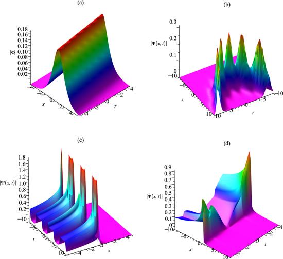
Figure 1. The wave intensity: (a) ∣ψ∣ of (21) with the parameters $\upsilon =1,{\rm{\Upsilon }}=\tfrac{-1}{2},\delta =1,r=2,\alpha =1,\beta =1$ and the arbitrary functions X = ax, a = 1, β(t) = 1, r(t) = 0; (b) ∣ψ∣ of (22) with the parameters $\upsilon =1,{\rm{\Upsilon }}=\tfrac{-1}{2},\delta =1,r=2,\alpha =1,\beta =1$ and the arbitrary functions X = ax, a = 1, β(t) = t, r(t) = 1; (c)∣ψ∣ of (22) with the parameters $\upsilon =1,{\rm{\Upsilon }}=1,\delta =1,r=\tfrac{-1}{4},\alpha =\tfrac{1}{3},\beta =\tfrac{1}{4}$ and the arbitrary functions $X={ax},a=1,\beta (t)={\rm{\cos }}(t),r(t)=100{\rm{\cos }}(t);$ (d) ∣ψ∣ of (22) with the parameters $\upsilon =1,{\rm{\Upsilon }}=1,\delta =1,r=\tfrac{-1}{4},\alpha =\tfrac{4}{3},\beta =\tfrac{1}{4}$ and the arbitrary functions $X={ax},a=1,\beta (t)={\rm{\cos }}(t),r(t)=100{\rm{\cos }}(t)$. |
According to the dark-soliton solution of equation (15 ) and the transformation (16 ), the nonautonomous one-dark soliton solution of equation (14 ) is presented with the extended sinh-Gordon equation
$\begin{eqnarray}\begin{array}{l}{{\rm{\Psi }}}_{D}(x,t)={\rho }_{0}{\left(\displaystyle \frac{\alpha -1}{\alpha }{\int }_{0}^{t}{\left(-\displaystyle \frac{r\left(t\right)}{\delta +2\,a\left(t\right)\varphi {\text{}}\_{t}^{\alpha }}\right)}^{{\alpha }^{-1}}\,{\rm{d}}t\right)}^{\tfrac{\alpha }{\alpha -1}}\\ \quad \times \,{{\rm{e}}}^{{\rm{i}}\varphi (x,t)}\left(-\sqrt{-\displaystyle \frac{2\,{\rm{\Upsilon }}\,{\delta }^{2}+2\,\upsilon }{4\,{r}^{2}{\upsilon }^{2}+4\,r\upsilon \,\delta +8\,\upsilon \,{\rm{\Upsilon }}+{\delta }^{2}}}\right.\\ \quad \times \,\left.\tanh \left(\displaystyle \frac{{X}^{\beta }}{\beta }+\displaystyle \frac{{{vT}}^{\alpha }}{\alpha }\right){{\rm{e}}}^{{\rm{i}}\left(\tfrac{{{pX}}^{\beta }}{\beta }+\displaystyle \frac{{{rT}}^{\alpha }}{\alpha }\right)}\right).\end{array}\end{eqnarray}$
In this particular case, we can derive the following fractional dark soliton $\begin{eqnarray}\begin{array}{l}{{\rm{\Psi }}}_{D}(x,t)={\rho }_{0}{{\rm{e}}}^{-{\int }_{0}^{t}\gamma (s){\rm{d}}{s}}{e}^{{\rm{i}}\varphi (x,t)}\\ \quad -\sqrt{-\displaystyle \frac{2\,{\rm{\Upsilon }}\,{\delta }^{2}+2\,\upsilon }{4\,{r}^{2}{\upsilon }^{2}+4\,r\upsilon \,\delta +8\,\upsilon \,{\rm{\Upsilon }}+{\delta }^{2}}}\\ \quad \times \,\tanh \left(\displaystyle \frac{{X}^{\beta }}{\beta }+\displaystyle \frac{{{vT}}^{\alpha }}{\alpha }\right){{\rm{e}}}^{{\rm{i}}\left(\tfrac{{{pX}}^{\beta }}{\beta }+\displaystyle \frac{{{rT}}^{\alpha }}{\alpha }\right)},\end{array}\end{eqnarray}$
with X(x, t) = ax, $T(t)={\int }_{0}^{t}-{\left(\tfrac{{a}^{2}\beta \left(t\right)}{{\rm{\Upsilon }}}\right)}^{{\alpha }^{-1}}\,{\rm{d}}t$, $\nu =-\tfrac{2\,p{\rm{\Upsilon }}+1}{2\,r\upsilon +\delta }$,$P=-\tfrac{4\,{r}^{2}{\upsilon }^{2}+8\,\upsilon \,{\rm{\Upsilon }}+4\,r\upsilon \,\delta +{\delta }^{2}}{2{\rm{\Upsilon }}\left(4\,{r}^{2}{\upsilon }^{2}+4\,r\upsilon \,\delta +8\,\upsilon \,{\rm{\Upsilon }}+{\delta }^{2}\right)}$$\,\tfrac{\sqrt{-{\left(2\,r\left(4\,{r}^{2}{\upsilon }^{2}+4\,r\upsilon \,\delta +8\,\upsilon \,{\rm{\Upsilon }}+{\delta }^{2}\right)\upsilon \left(4\,{r}^{2}{\upsilon }^{2}+4\,r\upsilon \,\delta +8\,\upsilon \,{\rm{\Upsilon }}+{\delta }^{2}\right)+\delta \left(4\,{r}^{2}{\upsilon }^{2}+4\,r\upsilon \,\delta +8\,\upsilon \,{\rm{\Upsilon }}+{\delta }^{2}\right)\right)}^{2}\left(-1+4\,{\rm{\Upsilon }}\left(2\,{\rm{\Upsilon }}+r\left(r\upsilon +\delta \right)\right)\right)}}{2{\rm{\Upsilon }}\left(4\,{r}^{2}{\upsilon }^{2}+4\,r\upsilon \,\delta +8\,\upsilon \,{\rm{\Upsilon }}+{\delta }^{2}\right)}.$
Figure 2 is plotted to describe the wave propagation of fractional nonautonomous one-dark soliton solution (24 ). From the comparison between figures 2(a) and (b), the function β(t) has no effect on the wave shapes, and the wave shapes are invariant during the propagation with two functions β(t). However, the wave periods have an effect on a function γ(t) and two parameters α, β. The linear type soliton is also shown in figure 2(a), and the parabolic type soliton is obtained in figure 2(b). It is clear that the breather-kink type soliton solution can be obtained by changing the fractional parameters α and β, and the ‘h’ -periodic solution can be obtained by choosing the special values β(t) and γ(t), which can increase or decrease the amplitudes of the solitary pattern solutions in figures 2(c) and (d). We obtain the non-autonomous one-dark soliton when we choose the different functions. The surface graphs of equation (14 ) are different from the results of previous work.
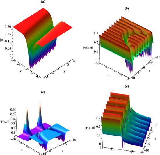
Figure 2. The wave intensity: (a) ∣ψ∣ of (23) with the parameters $\upsilon =1,{\rm{\Upsilon }}=\tfrac{-1}{2},\delta =1,r=2,\alpha =1,\beta =1$ and the arbitrary functions X = ax, a = 1, β(t) = 1, r(t) = 0; (b) ∣ψ∣ of (24) with the parameters $\upsilon =1,{\rm{\Upsilon }}=\tfrac{-1}{2},\delta =1,r=2,\alpha =1,\beta =1$ and the arbitrary functions $X={ax},a=1,\beta (t)=t,r(t)={\sin }(3t);$ (c)∣ψ∣ of (24) with the parameters $\upsilon =1,{\rm{\Upsilon }}=-\tfrac{1}{2},\delta =1,r=2,\alpha =\tfrac{1}{3},\beta =\tfrac{1}{4}$ and the arbitrary functions $X={ax},a=1,\beta (t)=t,r(t)={\sin }(2t);$ (d) ∣ψ∣ of (24) with the parameters $\upsilon =1,{\rm{\Upsilon }}=-\tfrac{1}{2},\delta =1,r=2,\alpha =1,\beta =\tfrac{1}{4}$ and the arbitrary functions $X={ax},a=1,\beta (t)={\rm{\cos }}(t),r(t)={\rm{\cos }}(2t)$. |
5. Nonautonomous bright–dark soliton solution and interaction for FGP equation
The soliton dynamics and some interactions of the FGP equation with some free functions have few results. We will analyze some soliton dynamics of the NBDSs for the FGP equation in (14 ) with some management functions β(t) and γ(t), which are different from the work in some previous studies
According to some bright–dark solitons (BDSs) of equation (15 ) and the transformation method (16 ), we obtain the fractional nonautonomous BDSs and combined singular soliton solutions of equation (14 ) in the following form
$\begin{eqnarray}\begin{array}{l}{{\rm{\Psi }}}_{{BD}}(x,t)={\rho }_{0}{\left(\displaystyle \frac{\alpha -1}{\alpha }{\int }_{0}^{t}{\left(-\displaystyle \frac{r\left(t\right)}{\delta +2\,a\left(t\right)\varphi {\text{}}\_{t}^{\alpha }}\right)}^{{\alpha }^{-1}}\,{\rm{d}}t\right)}^{\tfrac{\alpha }{\alpha -1}}\\ \quad \times \,{{\rm{e}}}^{{\rm{i}}\varphi (x,t)}\sqrt{-\displaystyle \frac{{\rm{\Upsilon }}\,{\delta }^{2}+\upsilon }{8\,{r}^{2}{\upsilon }^{2}+8\,r\upsilon \,\delta +4\,\upsilon \,{\rm{\Upsilon }}+2\,{\delta }^{2}}}\\ \quad \times \,\left({\rm{sech}} \left(\displaystyle \frac{{X}^{\beta }}{\beta }+\displaystyle \frac{{{vT}}^{\alpha }}{\alpha }\right)+\tanh \left(\displaystyle \frac{{X}^{\beta }}{\beta }+\displaystyle \frac{{{vT}}^{\alpha }}{\alpha }\right)\right){{\rm{e}}}^{{\rm{i}}\left(\tfrac{{{pX}}^{\beta }}{\beta }+\displaystyle \frac{{{rT}}^{\alpha }}{\alpha }\right)},\end{array}\end{eqnarray}$
and the combined singular soliton solution of the FGP equation $\begin{eqnarray}\begin{array}{l}{{\rm{\Psi }}}_{{CS}}(x,t)={\rho }_{0}{\left(\displaystyle \frac{\alpha -1}{\alpha }{\int }_{0}^{t}{\left(-\displaystyle \frac{r\left(t\right)}{\delta +2\,a\left(t\right)\varphi {\text{}}\_{t}^{\alpha }}\right)}^{{\alpha }^{-1}}\,{\rm{d}}t\right)}^{\tfrac{\alpha }{\alpha -1}}\\ \quad \times \,{{\rm{e}}}^{{\rm{i}}\varphi (x,t)}\sqrt{-\displaystyle \frac{{\rm{\Upsilon }}\,{\delta }^{2}+\upsilon }{8\,{r}^{2}{\upsilon }^{2}+8\,r\upsilon \,\delta +4\,\upsilon \,{\rm{\Upsilon }}+2\,{\delta }^{2}}}\\ \quad \times \,\left(\coth \left(\displaystyle \frac{{X}^{\beta }}{\beta }+\displaystyle \frac{{{vT}}^{\alpha }}{\alpha }\right)\right.\\ \quad \left.+{csch}\left(\displaystyle \frac{{X}^{\beta }}{\beta }+\displaystyle \frac{{{vT}}^{\alpha }}{\alpha }\right)\right){{\rm{e}}}^{{\rm{i}}\left(\tfrac{{{pX}}^{\beta }}{\beta }+\displaystyle \frac{{{rT}}^{\alpha }}{\alpha }\right)},\end{array}\end{eqnarray}$
where X(x, t) = ax, $T(t)={\int }_{0}^{t}-{\left(\tfrac{{a}^{2}\beta \left(t\right)}{{\rm{\Upsilon }}}\right)}^{{\alpha }^{-1}}\,{\rm{d}}t$, $\nu =-\tfrac{2\,p{\rm{\Upsilon }}+1}{2\,r\upsilon +\delta }$,$P=-1/2\,\tfrac{4\,{r}^{2}{\upsilon }^{2}+4\,r\upsilon \,\delta +2\,\upsilon \,{\rm{\Upsilon }}+{\delta }^{2}}{{\rm{\Upsilon }}\left(4\,{r}^{2}{\upsilon }^{2}+4\,r\upsilon \,\delta -4\,\upsilon \,{\rm{\Upsilon }}+{\delta }^{2}\right)}$$1/2\,\tfrac{\sqrt{-{\left(2\,r\left(4\,{r}^{2}{\upsilon }^{2}+4\,r\upsilon \,\delta +2\,\upsilon \,{\rm{\Upsilon }}+{\delta }^{2}\right)\upsilon \left(4\,{r}^{2}{\upsilon }^{2}+4\,r\upsilon \,\delta +2\,\upsilon \,{\rm{\Upsilon }}+{\delta }^{2}\right)+\delta \left(4\,{r}^{2}{\upsilon }^{2}+4\,r\upsilon \,\delta +2\,\upsilon \,{\rm{\Upsilon }}+{\delta }^{2}\right)\right)}^{2}\left(-1+2\,{\rm{\Upsilon }}\left({\rm{\Upsilon }}+2\,r\left(r\upsilon +\delta \right)\right)\right)}}{{\rm{\Upsilon }}\left(4\,{r}^{2}{\upsilon }^{2}+4\,r\upsilon \,\delta -4\,\upsilon \,{\rm{\Upsilon }}+{\delta }^{2}\right)}$.
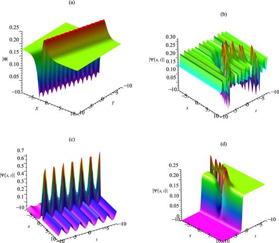
Similarly, several new optical solitons of space-time FGP equation with external potential (14 ) can be obtained in terms of elliptic functions by considering all the possible choices of α, β in equations (25 ) and (26 ). The corresponding bright–dark soliton solution and combined singular soliton solution can be found if we take the limit values, respectively. The BDSs propagate along the same direction on the x − t plane, which does not have the dynamics of interaction with the parameters α = 1, β = 1, r(t) = 0, β(t) = 1 in figure 3(a). Figure 3(b) shows the dynamic between two BDSs (parabolic-typed) propagating via the identical direction and some free functions β(t) and γ(t). And we can find the same shape as a ‘breather-like’ soliton on the periodic wave condition in figure 3(c). The corresponding parabolic-type bright and kink-type soliton solutions can be found if we take the fractional α, β values, meanwhile, the interaction between the obtained nonautonomous bright–dark soliton solution is illustrated in figure 3(d). Furthermore, the remarkable features of the fractional soliton wave solutions and phase portraits of the dynamical system are demonstrated through interesting figures. The geometric behaviors of equations (25 ) and (26 ) are investigated subsequently by choosing the different fractional parameters α, β of the FGP equation (14 ). We can study the evolution of nonautonomous soliton with exponential increasing and periodic changing nonlinearity, to show possibilities to manipulate them in nonautonomous nonlinear optics and Bose–Einstein condensate systems.
Figure 3. The plot: (a) the ∣ψ∣ of (25) with the parameters $\upsilon =1,{\rm{\Upsilon }}=\tfrac{-1}{2},\delta =1,r=2,\alpha =1,\beta =1$ and the arbitrary functions X = ax, a = 1, β(t) = 1, r(t) = 0; (b) ∣ψ∣ of (26) with the parameters $\upsilon =-1,{\rm{\Upsilon }}=\tfrac{1}{2},\delta =1,r=2,\alpha =1,\beta =1$ and the arbitrary functions $X={ax},a=1,\beta (t)=t,r(t)={\rm{\cos }}(4t);$ (c)∣ψ∣ of (26) with the parameters $\upsilon =1,{\rm{\Upsilon }}=-\tfrac{1}{2},\delta =1,r=2,\alpha =1,\beta =\tfrac{1}{2}$ and the arbitrary functions $X={ax},a=1,\beta (t)={\rm{\cos }}(t),r(t)={\rm{\cos }}(2t);$ (d) ∣ψ∣ of (26) with the parameters $\upsilon =-1,{\rm{\Upsilon }}=\tfrac{1}{2},\delta =1,r=2,\alpha \,=\tfrac{1}{3},\beta =1$ and the arbitrary functions X = ax, a = 1, β(t) = t2), r(t) = 1. |
6. Conclusions
In this paper, we derive the fractional nonautonomous bright–dark solutions and their controllable behaviors in the conformable space-time FGP equation with an external potential. We also consider the effect of α, β in nonautonomous bright–dark solutions of the space-time FGP equation. As a result, the novel shape bright soliton solution and novel “h”-shape dark soliton solution are presented, and we present the novel wave prolongs by controlling the fractional spatial–temporal part with α, β. Some novel solutions are obtained in this paper that have not been reported in previous studies. We can find there are some novel results in the fractional equation, and the improved method is a very powerful tool to solve the fractional differential equation. The reported result and method in our paper can help to obtain the meanings of some physical models. Based on the computations in our work, we observed that the applied integral scheme is a powerful and efficient mathematical tool and it provides encouragement for studying various complex fractional nonlinear models. Its concept can also be extended to other integrable fractional nonlinear evolution equations.