


1. Introduction
The universe in the beginning and future may have anisotropies despite the widely accepted assumption that the current universe is homogeneous and isotropic. In 1992, cosmic background explorer [1] revealed that the cosmic microwave background possesses a small amount of anisotropy at cosmological scales. The observational evidence, such as Wilkinson microwave anisotropy probe experiments [2] and cosmic background imager [3], strongly support this anisotropic nature of spacetime geometry. In 1998, the supernovae cosmology project led by Perlmutter and Riess confirmed the accelerating behavior of the Universe’s expansion [4, 5]. Moreover, recent advancements indicate the variations in the strengths of microwaves received from different directions, i.e. the Universe’s expansion is anisotropic [6]. One can efficiently describe the homogeneous and anisotropic nature of spacetime using Bianchi-type cosmology. Several models based on Bianchi cosmology have appeared in the literature [7–13]. In the present work, we incorporate locally rotationally symmetric (LRS) Bianchi type-I metric that is near to the Friedmann–Lemaître–Robertson–Walker (FLRW) metric and can be considered as a generalization of the isotropic one.
It is well known that the modified theories of gravity are capable of bypassing the undetected dark energy issue. The cosmological models based on the modifications of the Einstein action of general relativity that are obtained by introducing the function f(R) of the Ricci curvature R, first appeared in [14–16]. This cosmological model could describe the observed cosmic expansion without incorporating any dark energy component [17, 18]. Observational characteristics of f(R) gravity models, along with the constraints acquired by the equivalence principle and solar system tests, are investigated in the references [19–23]. The viable f(R) gravity models in the perspective of solar system tests do exist [24–26]. Odintsov et al have studied energy conditions and the H0 tension in the context of f(R) gravity models [27, 28]. One can follow references [29–35] to review some viable f(R) gravity models.
Bertolami et al [36] introduced a generalization of the f(R) modified gravity by assuming an explicit coupling between the generic f(R) function of the Ricci curvature scalar R and the Lagrangian density of matter Lm, in the Einstein–Hilbert action. T Harko and F S N Lobo further extended this model to the case of arbitrary geometry-matter couplings [37]. The cosmological models incorporating the non-minimal curvature and matter couplings present some interesting applications in cosmology and astrophysics [38–40]. Further, T Harko and F S N Lobo proposed [41] f(R, Lm) gravity, which is the set of all curvature-matter coupling theories. In this modified gravity, the energy-momentum tensor has the non-vanishing covariant divergence, an extra force orthogonal to four velocities arises, and the motion of the test particle is non-geodesic. Moreover, the f(R, Lm) modified theory of gravity does not satisfy the equivalence principle, and it is constrained by the solar system tests [42, 43]. Nowadays, plenty of interesting cosmological implications of f(R, Lm) gravity theory started appearing in the literature; for instance, check references [44–50].
In this manuscript, we investigate the bulk viscous matter dominated f(R, Lm) cosmological model with the anisotropic background. The significance of viscosity coefficients in cosmological modeling has a long history. From the hydrodynamics perspective, whenever a system loses its thermal equilibrium state, an effective pressure is generated to retrieve its thermal stability. Bulk viscosity in a matter content of the cosmos can be viewed as a manifestation of such an effective pressure. We aim to investigate the impact on the evolution phase of the Universe when we consider the effect of bulk viscosity coefficient ζ in the usual cosmic pressure. We assume that the coefficient of viscosity ζ obeys a scaling law, and that reduces the Einstein case to a form proportional to the Hubble parameter [51]. This scaling law considered in our study is quite useful. One can follow references to review some attractive cosmological models incorporating the viscosity in cosmic fluid [52–58].
The present work is organized as follows. In section 2 , we present the fundamental formulations of f(R, Lm) gravity. In section 3 , we derive the field equations corresponding to the LRS Bianchi type I metric. Further, we consider a cosmological f(R, Lm) model and then obtain the Hubble parameter value in terms of cosmic redshift. In section 4 , we utilize the H(z) and Pantheon observational data to estimate the model and bulk viscous parameter values. In the next section 5 , we present the physical behavior of cosmological parameters and statefinder diagnostic corresponding to the values of parameters obtained by the H(z), Pantheon, and H(z)+Pantheon data. In addition, in section 6 , we investigate the different energy conditions. Finally, in section 7 , we discuss and conclude our results.
2. f(R, Lm) gravity theory
The action ruling the gravitational interactions in f(R, Lm) gravity is given as
$\begin{eqnarray}S=\int f(R,{L}_{m})\sqrt{-g}{{\rm{d}}}^{4}x.\end{eqnarray}$
Here f(R, Lm) is the generic function of the Ricci curvature R and the matter Lagrangian Lm.The Ricci curvature term R can be obtained by the following contraction,
$\begin{eqnarray}R={g}^{\mu \nu }{R}_{\mu \nu },\end{eqnarray}$
where Rμν is the Ricci tensor and it is defined as $\begin{eqnarray}{R}_{\mu \nu }={\partial }_{\lambda }{{\rm{\Gamma }}}_{\mu \nu }^{\lambda }-{\partial }_{\mu }{{\rm{\Gamma }}}_{\lambda \nu }^{\lambda }+{{\rm{\Gamma }}}_{\mu \nu }^{\lambda }{{\rm{\Gamma }}}_{\sigma \lambda }^{\sigma }-{{\rm{\Gamma }}}_{\nu \sigma }^{\lambda }{{\rm{\Gamma }}}_{\mu \lambda }^{\sigma },\end{eqnarray}$
with ${{\rm{\Gamma }}}_{\beta \gamma }^{\alpha }$ denoting the components of Levi-Civita connection.One can obtain the following field equation of f(R, Lm) gravity by varying the action (1 ) with respect to the metric gμν,4 )
$\begin{eqnarray}{f}_{R}{R}_{\mu \nu }+({g}_{\mu \nu }\,\square -{{\rm{\nabla }}}_{\mu }{{\rm{\nabla }}}_{\nu }){f}_{R}-\displaystyle \frac{1}{2}(f-{f}_{{L}_{m}}{L}_{m}){g}_{\mu \nu }=\displaystyle \frac{1}{2}{f}_{{L}_{m}}{T}_{\mu \nu },\end{eqnarray}$
where ${f}_{R}\equiv \tfrac{\partial f}{\partial R}$, ${f}_{{L}_{m}}\equiv \tfrac{\partial f}{\partial {L}_{m}}$, and Tμν is the energy momentum tensor given by $\begin{eqnarray}{T}_{\mu \nu }=\displaystyle \frac{-2}{\sqrt{-g}}\displaystyle \frac{\delta (\sqrt{-g}{L}_{m})}{\delta {g}^{\mu \nu }}.\end{eqnarray}$
One can acquire the following relation by contracting the field equation ( $\begin{eqnarray}{{Rf}}_{R}+3\,\square {f}_{R}-2(f-{f}_{{L}_{m}}{L}_{m})=\displaystyle \frac{1}{2}{f}_{{L}_{m}}T.\end{eqnarray}$
Here R, T, and Lm being the Ricci curvature scalar, energy-momentum scalar, and the matter Lagrangian term respectively. Furthermore, $\square F=\tfrac{1}{\sqrt{-g}}{\partial }_{\alpha }(\sqrt{-g}{g}^{\alpha \beta }{\partial }_{\beta }F)$ for any scalar function F.
Moreover, by employing the covariant derivative in equation (4 ) one can obtain the following relation
$\begin{eqnarray}{{\rm{\nabla }}}^{\mu }{T}_{\mu \nu }=2{{\rm{\nabla }}}^{\mu }{ln}({f}_{{L}_{m}})\displaystyle \frac{\partial {L}_{m}}{\partial {g}^{\mu \nu }}.\end{eqnarray}$
3. The cosmological f(R, Lm) model with anisotropic background
Taking into account anomalies found in the observations of CMB, we consider following the LRS Bianchi type-I metric to describe the spatially homogeneous and anisotropic nature of the Universe8 ), we obtained the Ricci scalar as
$\begin{eqnarray}{\rm{d}}{s}^{2}=-{\rm{d}}{t}^{2}+{A}^{2}(t){\rm{d}}{x}^{2}+{B}^{2}(t)({\rm{d}}{y}^{2}+{\rm{d}}{z}^{2}),\end{eqnarray}$
where A(t) and B(t) are time dependent metric potentials. In particular, one can recover the usual flat FLRW background for A(t) = B(t) = a(t). Now, for the line element ( $\begin{eqnarray}R=2(\dot{{H}_{x}}+2\dot{{H}_{y}})+2({{H}_{x}}^{2}+3{{H}_{y}}^{2})+4{H}_{x}{H}_{y}.\end{eqnarray}$
Here ${H}_{x}=\tfrac{\dot{A}}{A}$ and ${H}_{y}={H}_{z}=\tfrac{\dot{B}}{B}$ represents directional Hubble parameters.The stress-energy tensor characterizing the Universe filled with viscous content reads as
$\begin{eqnarray}{T}_{\mu \nu }=(\rho +\bar{p}){u}_{\mu }{u}_{\nu }+\bar{p}{g}_{\mu \nu },\end{eqnarray}$
where $\bar{p}=p-3\zeta H$ denotes the effective pressure of the cosmic fluid in the presence of viscosity coefficient ζ and ρ is the usual matter energy density with four velocities components uμ = (1, 0, 0, 0).The field equations governing the dynamics of the viscous matter dominated universe in f(R, Lm) with anisotropic background reads as
$\begin{eqnarray}\begin{array}{l}(2{H}_{x}{H}_{y}+{{H}_{y}}^{2}){f}_{R}+\displaystyle \frac{1}{2}(f-{{Rf}}_{R}-{L}_{m}{f}_{{L}_{m}})\\ \quad +\dot{{f}_{R}}({H}_{x}+2{H}_{y})=\displaystyle \frac{1}{2}{f}_{{L}_{m}}\rho ,\end{array}\end{eqnarray}$
$\begin{eqnarray}\begin{array}{l}(\dot{{H}_{x}}+{{H}_{x}}^{2}+2{H}_{x}{H}_{y}){f}_{R}-\ddot{{f}_{R}}-\dot{{f}_{R}}({H}_{x}+2{H}_{y})\\ \quad -\displaystyle \frac{1}{2}(f-{L}_{m}{f}_{{L}_{m}})=\displaystyle \frac{1}{2}{f}_{{L}_{m}}\bar{p},\end{array}\end{eqnarray}$
$\begin{eqnarray}\begin{array}{l}(\dot{{H}_{y}}+2{{H}_{y}}^{2}+{H}_{x}{H}_{y}){f}_{R}-\ddot{{f}_{R}}-\dot{{f}_{R}}({H}_{x}+2{H}_{y})\\ \quad -\displaystyle \frac{1}{2}(f-{L}_{m}{f}_{{L}_{m}})=\displaystyle \frac{1}{2}{f}_{{L}_{m}}(\bar{p}+\delta \rho ).\end{array}\end{eqnarray}$
Here δ is a measure of deviation from isotropy along y and z axes, called the skewness parameter.
In this work, we study the following f(R, Lm) model in order to explore the cosmological implications of the f(R, Lm) gravity [62, 63],
$\begin{eqnarray}f(R,{L}_{m})=\displaystyle \frac{R}{2}+{L}_{m}^{\alpha },\end{eqnarray}$
where α is an arbitrary parameter. The cosmological f(R, Lm) model that we have considered is motivated by the generic function f(R, Lm) = f1(R) + f2(R)G(Lm) that represents arbitrary curvature-matter coupling [63]. In particular, for α = 1 one can obtain the usual Friedmann equations of GR.Now one can acquire the spatial volume element as15 ), the mean value of the Hubble parameter can be calculated as
$\begin{eqnarray}V={{AB}}^{2}.\end{eqnarray}$
Then by using ( $\begin{eqnarray}H=\displaystyle \frac{1}{3}\displaystyle \frac{\dot{V}}{V}=\displaystyle \frac{1}{3}({H}_{x}+2{H}_{y}).\end{eqnarray}$
Further, we consider an extra ansatz to obtain the exact solution of the field equations. We consider a physical relation between the expansion scalar θ and shear scalar Σ, specifically, θ2 ∝ Σ2 . In particular, for $\tfrac{\sigma }{\theta }=\mathrm{constant}$, one can retrieve the isotropy of Hubble expansion [64]. This gives rise to a following relation
$\begin{eqnarray}A={B}^{n},\end{eqnarray}$
and the corresponding directional Hubble parameter can be obtained as $\begin{eqnarray}{H}_{x}={{nH}}_{y},n\ne 0.\end{eqnarray}$
For n = 1, one can recover the usual flat FLRW cosmology.Now, for the specific function (14 ) with Lm = ρ [65], we obtained the following Friedmann equations for a non-relativistic viscous matter dominated universe, by using equations (11 )–(13 )
$\begin{eqnarray}(2n+1){{H}_{y}}^{2}=(2\alpha -1){\rho }^{\alpha },\end{eqnarray}$
$\begin{eqnarray}2\dot{{H}_{y}}+3{{H}_{y}}^{2}=(\alpha -1){\rho }^{\alpha }-\alpha {\rho }^{\alpha -1}\bar{p},\end{eqnarray}$
$\begin{eqnarray}\begin{array}{l}(n+1)\dot{{H}_{y}}+({n}^{2}+n+1){{H}_{y}}^{2}\\ \quad =(\alpha -1){\rho }^{\alpha }-\alpha {\rho }^{\alpha -1}(\bar{p}+\delta \rho ).\end{array}\end{eqnarray}$
By using equations (19 ) and (20 ), we obtain following first-order equation
$\begin{eqnarray}\begin{array}{l}\dot{{H}_{y}}+\left[\displaystyle \frac{5\alpha -2+2n(1-\alpha )}{2(2\alpha -1)}\right]{H}_{y}^{2}\\ \quad =\displaystyle \frac{\alpha \zeta }{2}(n+2){\left(\displaystyle \frac{2n+1}{2\alpha -1}\right)}^{\tfrac{\alpha -1}{\alpha }}{{H}_{y}}^{\tfrac{3\alpha -2}{\alpha }}.\end{array}\end{eqnarray}$
On integrating the above equation, we have
$\begin{eqnarray}\begin{array}{l}{H}_{y}=\left\{{H}_{{y}_{0}}^{\tfrac{2-\alpha }{\alpha }}{\left(1+z\right)}^{\tfrac{(2-\alpha )[5\alpha -2+2n(1-\alpha )]}{2\alpha (2\alpha -1)}}\right.\\ \quad +\displaystyle \frac{\alpha \xi (n+2){\left(2\alpha -1\right)}^{\tfrac{1}{\alpha }}{\left(2n+1\right)}^{\tfrac{\alpha -1}{\alpha }}}{5\alpha -2+2n(1-\alpha )}\\ \quad {\left.\times \left[1-{\left(1+z\right)}^{\tfrac{(2-\alpha )[5\alpha -2+2n(1-\alpha )]}{2\alpha (2\alpha -1)}}\right]\right\}}^{\tfrac{\alpha }{2-\alpha }}.\end{array}\end{eqnarray}$
Here ${H}_{y}(0)={H}_{{y}_{0}}$. Now by using equations (16 ) and (18 ), we obtained the average value of the Hubble parameter as24 ) in (23 ), we obtained the expression for averaged Hubble parameter in terms of redshift as
$\begin{eqnarray}H=\left(\displaystyle \frac{n+2}{3}\right){H}_{y}.\end{eqnarray}$
By using equations ( $\begin{eqnarray}\begin{array}{l}H(z)=\left(\displaystyle \frac{n+2}{3}\right)\left\{{\left(\displaystyle \frac{3{H}_{0}}{n+2}\right)}^{\tfrac{2-\alpha }{\alpha }}{\left(1+z\right)}^{\tfrac{(2-\alpha )[5\alpha -2+2n(1-\alpha )]}{2\alpha (2\alpha -1)}}\right.\\ \quad +\displaystyle \frac{\alpha \xi (n+2){\left(2\alpha -1\right)}^{\tfrac{1}{\alpha }}{\left(2n+1\right)}^{\tfrac{\alpha -1}{\alpha }}}{5\alpha -2+2n(1-\alpha )}\\ \quad {\left.\times \left[1-{\left(1+z\right)}^{\tfrac{(2-\alpha )[5\alpha -2+2n(1-\alpha )]}{2\alpha (2\alpha -1)}}\right]\right\}}^{\tfrac{\alpha }{2-\alpha }},\end{array}\end{eqnarray}$
where H(0) = H0 is the present value of the Hubble parameter.4. Observational constraints
In this section, we are going to investigate the viability of our theoretical model by utilizing observational data sets. In this work, we incorporate updated H(z) data sets and the Pantheon supernovae observations. In order to perform statistical analysis, we use the χ2 minimization technique along with the Markov Chain Monte Carlo random sampling method in the emcee python library [66].
4.1. H(z) datasets
It is well known that the expansion of the Universe can be characterized by the Hubble parameter. For early passively evolving galaxies, one can recover the Hubble parameter values by measuring the dt at a definite redshift value. In this work, we use 57 points of H(z) data in the redshift range 0.07 ≤ z ≤ 2.41 [67]. Moreover, there are two well-known approaches to extracting the values of the Hubble parameter, namely the differential age and line of sight baryonic acoustic oscillations method. The set of 57 H(z) data points can be checked in the reference [68, 69]. Now, the chi-square function corresponding to H(z) data points reads as
$\begin{eqnarray}{\chi }_{H}^{2}({H}_{0},\alpha ,\zeta ,n)=\displaystyle \sum _{k=1}^{57}\frac{{\left[{H}_{\mathrm{th}}({z}_{k},{H}_{0},\alpha ,\zeta ,n)-{H}_{\mathrm{obs}}({z}_{k})\right]}^{2}}{{\sigma }_{H({z}_{k})}^{2}},\end{eqnarray}$
where, the theoretically predicted value of the H(z) is denoted by Hth whereas Hobs represents the observed value of H(z) with standard error ${\sigma }_{H({z}_{k})}$. The contour plot for the model parameters α, ζ, n, and H0 corresponding to H(z) data sets at 1−Σ and 2−Σ confidence intervals is presented in figure 1.
Figure 1. The 1−Σ and 2−Σ contour plot for the model parameters using the H(z) data set. |
The obtained best fit values are $\alpha ={0.903}_{-0.10}^{+0.091}$, $\zeta ={180.006}_{-0.10}^{+0.092}$, n = 0.195 ± 0.096, and H0 = 66.499 ± 0.097.
4.2. Pantheon datasets
In this work, we incorporate 1048 points of Pantheon supernovae samples with corresponding distance moduli μobs in the redshift range z ∈ [0.01, 2.3] [70]. The χ2 function corresponding to Pantheon data sets is given as
$\begin{eqnarray}{\chi }_{{SN}}^{2}=\displaystyle \sum _{i,j=1}^{1048} \triangledown {\mu }_{i}{\left({C}_{{SN}}^{-1}\right)}_{{ij}} \triangledown {\mu }_{j},\end{eqnarray}$
Here CSN denotes the covariance matrix [70], and $\begin{eqnarray*} \triangledown {\mu }_{i}={\mu }^{\mathrm{th}}({z}_{i},\theta )-{\mu }_{i}^{\mathrm{obs}}.\end{eqnarray*}$
is the difference between the value of distance modulus obtained from the cosmological observations and its theoretically predicted values estimated from the given model with parameter space θ. One can estimate the distance modulus by using the relation μ = mB − MB, where mB and MB are the observed apparent magnitude and the absolute magnitude at a given redshift (Retrieving the nuisance parameter following the recent approach called BEAMS with Bias Correction [71]). Moreover, its theoretical value can be calculated as $\begin{eqnarray}\mu (z)=5{\mathrm{log}}_{10}\left[\frac{{D}_{L}(z)}{1\mathrm{Mpc}}\right]+25,\end{eqnarray}$
where $\begin{eqnarray}{D}_{L}(z)=c(1+z){\int }_{0}^{z}\displaystyle \frac{{dx}}{H(x,\theta )}.\end{eqnarray}$
The contour plot for the model parameters α, ζ, n, and H0 corresponding to Pantheon data sets at 1−Σ and 2−Σ confidence interval is presented in figure 2.
Figure 2. The 1−Σ and 2−Σ contour plot for the model parameters using the Pantheon data set. |
The obtained best fit values are α = 0.899 ± 0.098, ζ = 179.99 ± 0.10, n = 0.196 ± 0.098, and H0 = 66.498 ± 0.097.
4.3. H(z)+Pantheon datasets
The χ2 function to obtain the mean value of the model parameters corresponding to the combined H(z)+Pantheon data sets reads as
$\begin{eqnarray}{\chi }_{\mathrm{total}}^{2}={\chi }_{H}^{2}+{\chi }_{{SN}}^{2}.\end{eqnarray}$
The contour plot for the model parameters α, ζ, n, and H0 corresponding to H(z)+Pantheon data sets at 1−Σ and 2−Σ confidence interval is presented in figure 3.

Figure 3. The 1−Σ and 2−Σ contour plot for the model parameters using the H(z)+Pantheon data set. |
The obtained best fit values are α = 0.895 ± 0.098, ζ = 180.007 ± 0.099, n = 0.195 ± 0.099, and H0 = 66.50 ± 0.10.
5. Behavior of physical parameters
In this section, we are going to present the behavior of physical parameters that describes the evolution phase of the Universe, corresponding to the extracted values of the model parameters from different observational data sets.
The evolution profile of the matter-energy density and the effective pressure is presented in figures 4 and 5, respectively. We observe that the energy density indicates expected positive behavior, whereas pressure with viscosity coefficient shows negative behavior on the entire domain. Therefore the presence of the viscosity coefficient in the cosmic content contributes to the Universe’s expansion. The profile of the skewness parameter presented in figure 6 shows the anisotropic nature of the spacetime during the entire evolution phase of the Universe. Further, the effective EoS parameter presented in figure 7 favors the accelerating phase of the Universe’s expansion. Its present value corresponding to H(z), Pantheon, and combine H(z)+Pantheon data sets are ω0 ≈ −0.9, ω0 ≈ −0.85, and ω0 ≈ −0.8 respectively.

Figure 4. Profile of the matter-energy density vs cosmic redshift z. |

Figure 5. Profile of the effective pressure vs cosmic redshift z. |

Figure 6. Profile of the skewness parameter vs cosmic redshift z. |

Figure 7. Profile of the effective EoS vs cosmic redshift z. |
The statefinder diagnostic proposed by V Sahni [72] can geometrically differentiate different models of dark energy through statefinder parameters which are defined as
$\begin{eqnarray}r=\displaystyle \frac{\dddot{a}}{{{aH}}^{3}},\end{eqnarray}$
and $\begin{eqnarray}s=\displaystyle \frac{(r-1)}{3(q-\tfrac{1}{2})}.\end{eqnarray}$
The value (r > 1, s < 0) represents a phantom scenario whereas (r < 1, s > 0) denotes the quintessence type dark energy, and the value (r = 1, s = 0) mimics the standard ΛCDM model. The behavior of our f(R, Lm) model in the presence of viscous fluid in the r−s plane is presented in figure 8. The present values of statefinder parameters corresponding to H(z), Pantheon, and combine H(z)+Pantheon data sets are (r, s) = (0.87, 0.06), (r, s) = (0.82, 0.09), and (r, s) = (0.77, 0.12) respectively [73]. We found that our cosmological f(R, Lm) model lies in the quintessence region, and it behaves like the de-Sitter universe in the far future.

Figure 8. Profile of evolutionary trajectories of the given model in the r−s plane. |
6. Energy conditions
In this section, we investigate different energy conditions in order to test the consistency of the obtained solution of our model. The energy conditions are relations imposed on the energy-momentum tensor in order to satisfy positive energy. The energy conditions are obtained from the well-known Raychaudhuri equation and are written as [74]
with ρeff being the effective energy density.
| • | Null energy condition (NEC) : ρeff + peff ≥ 0; |
| • | Weak energy condition (WEC) : ρeff ≥ 0 and ρeff + peff ≥ 0; |
| • | Dominant energy condition (DEC) : ρeff ± peff ≥ 0; |
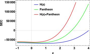
| • | Strong energy condition (SEC) : ρeff + 3peff ≥ 0, |
The profile of the NEC and the DEC with respect to cosmic redshift is presented in figures 9 and 10, respectively. Since WEC is the combination of NEC and the positive energy density, we found that corresponding to the extracted values of the model parameters from different observational data sets, NEC, DEC, and WEC shows positive behavior, whereas SEC presented in figure 11 favors a transition from positive to negative behavior in the recent past. Thus, the violation of SEC strongly supports the recently observed acceleration with the transition from decelerated to the accelerated phase of the Universe’s expansion in the recent past.

Figure 9. Profile of the null energy condition vs cosmic redshift z. |
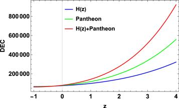
Figure 10. Profile of the dominant energy condition vs cosmic redshift z. |
Figure 11. Profile of the strong energy condition vs cosmic redshift z. |
7. Conclusion
From the hydrodynamics perspective, the assumption of viscous effects in the cosmic fluid is quite natural since the perfect fluid is, after all, an abstraction. In this work, we investigated the significance of viscosity coefficients to describe the observed cosmic acceleration by taking into account a cosmological f(R, Lm) model with an anisotropic background. We considered $f(R,{L}_{m})=\tfrac{R}{2}+{L}_{m}^{\alpha }$, where α is an arbitrary parameter, with the effective equation of state $\bar{p}=p-3\zeta H$ that is the Einstein case value with proportionality constant ζ used in the Einstein theory [51]. In section 3 , we obtained the analytical expression of the Hubble parameter H(z) by incorporating the assumed f(R, Lm) viscous fluid model. Further, in section 4 , we analyzed the viability of the assumed f(R, Lm) model by incorporating the observational data sets, specifically, H(z) data sets and the Pantheon supernovae data sets. The obtained best fit values are $\alpha ={0.903}_{-0.10}^{+0.091}$, $\zeta ={180.006}_{-0.10}^{+0.092}$, n = 0.195 ± 0.096, and H0 = 66.499 ± 0.097 for the H(z) datasets, α = 0.899 ± 0.098, ζ = 179.99 ± 0.10, n = 0.196 ± 0.098, and H0 = 66.498 ± 0.097 for the Pantheon datasets, and α = 0.895 ± 0.098, ζ = 180.007 ± 0.099, n = 0.195 ± 0.099, and H0 = 66.50 ± 0.10 [75] for the combined H(z)+Pantheon datsets. In section 5 , the behavior of some cosmological parameters has been presented. We observed that the energy density presented in figure 4 decreases with the expansion of the Universe, whereas the bulk viscous pressure presented in figure 5 indicates the negative behavior. The skewness parameter presented in figure 6 favors the anisotropic type evolution of the Universe during the entire time regime. Further, the effective EoS parameter in figure 7 shows the accelerating nature of the cosmic expansion with the present values ω0 ≈ −0.9, ω0 ≈ −0.85, and ω0 ≈ −0.8 corresponding to H(z), Pantheon, and the combined H(z)+Pantheon data sets respectively. Finally, from figure 8 we found that our cosmological f(R, Lm) model exhibits quintessence behavior, and it favors the de-Sitter type expansion in the far future. In section 6 , energy conditions have been analyzed to interpret the viability of the obtained solution. All energy conditions except SEC exhibit positive behavior (see figures 9 and 10), whereas the violation of SEC presented in figure 11 strongly supports the accelerating nature of cosmic expansion with the transition from decelerated to accelerated era.