


1. Introduction
The Kagome lattice is a two-dimensional hexagonal network composed of corner-sharing triangles, the structure of which has received considerable attention from the scientific community since its inception. This lattice can bind electrons in a six-membered ring and generate flat bands, thereby introducing interesting physical phenomena in condensed-matter physics. For example, when the Fermi surface is on a flat band, the extremely high density of the electron states on this band allows the system to be spontaneously ferromagnetic, despite the small Coulomb interaction between the electrons [1–3]. Additionally, the flat band is a natural platform for the realization of the Wigner lattice [4, 5] because the kinetic quenching of, and interactions between, electrons are dominant in this band. In addition, the Kagome structure is applied to the studies on Bose–Einstein condensate [6], high-temperature fractional quantum Hall effect [4, 7, 8], high-temperature superconductivity [9, 10], and other properties based on flat bands.
Another important property of the Kagome lattice is its ability to generate frustrated spin [11, 12]. Frustrated spin systems frequently manifest as interesting physical phenomena associated with nontrivial spin orders. Therefore, this lattice has attracted much attention as an important method of studying spin-liquid or spin-ice systems. For example, research and analysis of a series of spin-liquid materials, such as Y3Cu9(OH)19Cl8, CaCu3(OH)6Cl2 · 0.6H2O, and YCu3(OH)6Cl3, were conducted by applying this lattice [13–16].
The experimental results associated with the preparation and study of Kagome structural materials are equally impressive. Szymczak et al experimentally measured the inelastic neutron scattering from Co3V2O8 single crystals and the electron paramagnetic resonance of Co2+ ions in Mg3V2O8 single crystals [17]. The authors concluded that the magnetic anisotropy of (M = Co, Ni, Mn) step oxides is mainly owing to single ions. Jiang et al [18] prepared two open-frame transition metal fluorophosphates, ${({\mathrm{NH}}_{4}){{\rm{M}}}_{3}({\mathrm{PO}}_{3}{\rm{F}})}_{2}({\mathrm{PO}}_{2}{{\rm{F}}}_{2}){{\rm{F}}}_{2}$ (M = Mn and Co), possessing Kagome lattices and found that the Kagome topology of the material exacerbates magnetic frustration and exhibits an antiferromagnetic ground state. Furthermore, Fe-Sn alloys are typical Kagome materials. Lin et al [19] experimentally combined scanning tunneling microscopy, angle-resolved photoelectron spectroscopy, and first-principles calculations to confirm the existence of a flat-band electronic structure in the quasi-dimensional Kagome compound ${\mathrm{Fe}}_{3}{\mathrm{Sn}}_{2}$. The existence of a magnetic Dirac semimetal was experimentally demonstrated for the first time by the authors.
Magnetic and thermodynamic properties are equally popular areas of investigation in the study of Kagome lattice materials. The magnetic behavior of two-dimensional decorated Kagome lattices in the Ising model was studied by Si et al [20]. Ananikian et al [21] investigated the magnetic properties and entanglement of fluid 3He in a Kagome lattice. Their results demonstrated that the system exhibited diverse magnetic behaviors depending on the exchange parameters. Yerzhakov et al [22] investigated the thermodynamic characteristics of geometrically frustrated ABC-stacked antiferromagnetic Kagome layer films using Metropolis Monte Carlo (MC) simulations. Soldatov [23] investigated the diluted antiferromagnetic Ising model in magnetic fields on Kagome lattices and discussed the similarities and differences in the resulting magnetization curves. Owing to its simple implementation and versatility, the Ising model is beneficial for studying the magnetic behavior of nanostructured systems [24–26]. In addition, MC simulations allow the study of the magnetic behaviors and magnetocaloric effects of nano-systems [27–30]. In our previous study, we successfully described the magnetic and thermodynamic properties of a nano-system using the Ising model [31–33]. Moreover, dynamic phase transitions and hysteresis loop behaviors have raised significant interest [34, 35]. This is because when a material is exposed to a dynamically-applied magnetic field (both biased and time-varying oscillatory fields), the system does not simultaneously respond to both fields, but the order of the magnetic moment depends on the oscillating field over time, leading to dynamic phase transitions [36, 37]. Vatansever and Polat [38] researched materials, including triangular lattice and ferromagnetic thin film systems, under biased and oscillating magnetic fields and found that the amplitude of the oscillating magnetic fields affected the dynamic critical properties of the system [39]. Ertaš et al observed the dynamic hysteresis line behaviors of Ising ferromagnetic systems and discussed the effect of temperature on exchange coupling and the dynamic hysteresis behaviors [40–42]. Cardona et al used the MC method to study the influence of relevant parameters, including the frequency and amplitude of the oscillating magnetic field, on the dynamic magnetic and thermodynamic properties of La2/3Ca1/3MnO3 under a time-dependent magnetic field [43]. Gallardo et al used an analytical approach to analyze the dynamic phase transition of the kinetic Ising model in mean field approximation and found that the time-independent field components are conjugate fields with ordered parameters [44]. Studies of dynamic phase transitions such as these are important in recent magnetic research. Although many advances have been made in the theoretical studies on the magnetism of Kagome structural lattices, most of these studies have focused on constant applied magnetic fields. Based on the MC simulations, Z. D. Vatansever studied the effect of system sizes on dynamic phase transition behaviors of the Kagome lattice in the presence of a square-wave oscillating magnetic field. The results indicate that the phase transition temperature increases with the increase in system size [45]. In this study, based on a fixed system size, we used MC simulations to demonstrate the dynamic magnetic properties and magnetocaloric effect of a single-layer Kagome lattice under dynamic magnetic fields.
The remainder of this paper is organized as follows. In section 2 , we describe the model applied and briefly introduce the MC simulation. In section 3 , we analyze the typical results obtained using the Kagome lattice model under different relevant parameters such as dynamic order, blocking temperature, internal energy, phase diagram and magnetocaloric effect. Finally, section 4 presents the conclusions of the study.
2. Model and Monte Carlo simulation
A schematic of a Kagome lattice is shown in figure 1. The lattice consists of two types of sublattices; the yellow and blue balls represent sublattices A and B, respectively. The dash-dotted lines represent the nearest-neighbor ferromagnetic exchange couplings J1 (>0). The dotted and solid lines represent the ferrimagnetic exchange couplings Js (<0) and J (<0), respectively. Considering that the exchange coupling, anisotropy, and external magnetic field have significant influences on the system, the Hamiltonian of the system can be given as
$\begin{eqnarray}\begin{array}{rcl}H & = & -{J}_{1}\displaystyle \sum _{{ij}}{\sigma }_{i}^{z}{\sigma }_{j}^{z}-{J}_{s}\displaystyle \sum _{m,i}{S}_{m}^{z}{\sigma }_{i}^{z}-J\displaystyle \sum _{n,i}{S}_{n}^{z}{\sigma }_{i}^{z}\\ & & -D\displaystyle \sum _{m}{({S}_{m}^{z})}^{2}-{D}_{1}\displaystyle \sum _{i}{({\sigma }_{i}^{z})}^{2}-h(t)\displaystyle \sum _{m,i}({S}_{m}^{z}+{\sigma }_{i}^{2}),\end{array}\end{eqnarray}$
where ${\sigma }_{i}^{z}$ and Smz represent spins ±3/2 and ±2, respectively. The anisotropies are expressed as D1 and D, respectively, and h(t) is the magnetic field, which is composed of time-dependent oscillating and time-independent magnetic fields. To simplify the calculation, in the following calculation process, J1 = 1 is taken as the unit. Therefore, h(t) is written as $\begin{eqnarray}h(t)={h}_{\mathrm{bias}}+{h}_{\mathrm{osc}}\sin (2\pi * t/\tau ),\end{eqnarray}$
where hbias denotes the value of the bias field, hosc and τ represent the amplitude and period of the time-dependent oscillating field, respectively, and t represents the time measured by the MC simulation per spin step.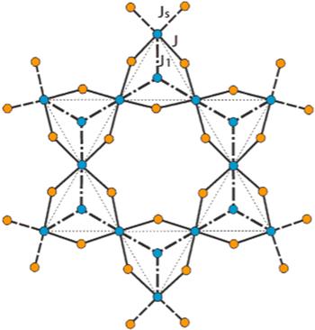
Figure 1. Diagram of the Kagome lattice. The yellow and blue balls represent magnetic atoms with spin −2 and spin −3/2, respectively. The dashed, solid and dash-dotted lines represent three types of exchange coupling Js, J, and J1, respectively. |
To simulate the magnetic properties of the Kagome model, we adopted the MC method based on the Metropolis algorithm [46]. To maintain the equilibrium of the system and ensure the reliability of the calculation results, we discarded the initial 3 × 10⁵ MC steps per spin and calculated the magnetic and thermodynamic quantities using the remaining 2 × 10⁵ MC steps. The system shown in figure 1 has 48 magnetic atoms divided into five sublattices (N1, N2, N3, N4, and N5). Sublattice A is composed of N1 and N3, and sublattice A is composed of N2, N4, and N5. The magnetizations per site are defined as
$\begin{eqnarray}\begin{array}{rcl}{M}_{A} & = & \frac{1}{{N}_{A}}\displaystyle \sum _{i=1}^{{N}_{A}}{S}_{i}^{z},\\ {M}_{B} & = & \frac{1}{{N}_{B}}\displaystyle \sum _{j=1}^{{N}_{B}}{\sigma }_{j}^{z},\end{array}\end{eqnarray}$
where NA is the number of sites in sublattices N1 and N3, and NB represents the number of sites in sublattices N2, N4, and N5. Therefore, we can evaluate the total magnetization of the system as $\begin{eqnarray}M=\displaystyle \frac{{N}_{A}{M}_{A}+{N}_{B}{M}_{B}}{{N}_{A}+{N}_{B}}.\end{eqnarray}$
The dynamic order parameters of the five sublattices are expressed as
$\begin{eqnarray}\begin{array}{rcl}{Q}_{A} & = & \displaystyle \frac{\omega }{2\pi }\oint {M}_{A}(t){\rm{d}}t,\\ {Q}_{B} & = & \displaystyle \frac{\omega }{2\pi }\oint {M}_{B}(t){\rm{d}}t.\end{array}\end{eqnarray}$
The dynamic order parameter is calculated as
$\begin{eqnarray}Q=\displaystyle \frac{{Q}_{A}{N}_{A}+{Q}_{B}{N}_{B}}{{N}_{A}+{N}_{B}}\quad (N=48).\end{eqnarray}$
We defined dynamic magnetic susceptibility as
$\begin{eqnarray}\chi =\displaystyle \frac{N}{{k}_{{\rm{B}}}T}(\langle {Q}^{2}\rangle -\langle Q{\rangle }^{2}).\end{eqnarray}$
The instantaneous internal energy per spin is calculated using
$\begin{eqnarray}E(t)=\displaystyle \frac{1}{2{N}^{2}}\langle H\rangle .\end{eqnarray}$
We can calculate the dynamical internal energy per spin as follows:
$\begin{eqnarray}U=\frac{\omega }{2\pi }\oint E(t),\end{eqnarray}$
where kB represents the Boltzmann constant, which we set to 1. The magnetic entropy of the system is calculated as follows: $\begin{eqnarray}S(T,h)={\int }_{{T}_{0}}^{T}\displaystyle \frac{C(T,h)}{T}{\rm{d}}T.\end{eqnarray}$
The magnetic entropy change can be expressed as
$\begin{eqnarray}{\rm{\Delta }}S(T,h)=S(T,h)-S(T,0).\end{eqnarray}$
For a magnetocaloric material, the relative cooling power (RCP) is an important factor and is given by
$\begin{eqnarray}\mathrm{RCP}={\int }_{{T}_{C}}^{{T}_{V}}{\rm{\Delta }}{S}_{m}(T){\rm{d}}T.\end{eqnarray}$
The temperatures at either end of the half-maximum value of ${\rm{\Delta }}{S}_{\max }$ are Tc and Tv, respectively.
3. Results and discussion
We demonstrated the influences of diverse parameters on dynamic thermodynamic quantities, such as Q, QA, QB, χ, and U on the Kagome lattice.
3.1. Dynamic order parameter, susceptibility, and internal energy
Figure 2 shows the variations in the dynamic order parameters of the system when the exchange-coupling J changes, and the remaining parameters are set to Js = −1.2, J1 = 1.0, hbias = 0.7, hosc = 1.1, D = −0.3, D1 = −0.6, and ω = 0.02π. Figure 2(a) shows the functional relationship between the average total dynamic order parameters (Q) and temperature (T) for different values of J. Only one saturation value (Qs =11/16) exists on all the Q −T curves. The curves begin at this value and then gradually decline to a constant value. The effects of J on Q are not obvious when T < 0.25 or T > 0.75. When 0.25 < T < 0.75, Q increases slowly with the increase in J. Moreover, for a certain T, the higher the J, the higher the Q, which indicates that strong exchange coupling accelerates the order energy of the system. From figure 2(b), the saturation values of QA and QB at T = 0, QA = 2.0, and QB = −1.5, can be observed. Therefore, QS = (30 × 2 + 18 × (−3/2))/48 = 11/16. Furthermore, QA and ∣QB∣ decrease with the increase in T, whereas QA and ∣QB∣ increase with the decrease in J, indicating that a high T or small J facilitates a disordered system. As shown in figure 2(c), every χ −Q curve has a maximum, which corresponds to the blocking temperature Tb, where Tb is a physical quantity that depends on ferromagnetic and antiferromagnetic (ferrimagnetic) materials. The system is in the ferromagnetic (ferrimagnetic) phase when T < Tb and in the paramagnetic phase when T > Tb. As T increases, the χ curves gradually shift to the high-temperature region. This behavior can be explained by an increase in the order energy of the system owing to the increase in J. Therefore, an increased amount of thermal energy is required to bring the system to disorder. In figure 2(d), the U curves are observed to increase as T increases and maintain a similar change rule. More specifically, when the temperature is low, U maintains a constant value. With the increase in T, U increases rapidly and subsequently slows. In addition, we observe that for the same temperature, U decreases as ∣J∣ increases.
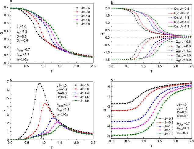
Figure 2. Temperature dependence of (a) the total dynamic order parameter Q, (b) dynamic order parameters QA and QB, (c) susceptibility χ, and (d) the internal energy U for various J with Js = −1.2, J1 = 1.0, D = −0.3, D1 = −0.6, hbias = 0.7, hosc = 1.1 and ω = 0.02π. |
Figure 3 shows the dynamic thermodynamic variables of the system when Js changes and the other parameters are fixed at J = −0.5, J1 = 1.0, hbias = 0.7, hosc =1.1, D = −0.3, D1 = −0.6, and ω = 0.02π. As shown in figure 3(a), the Q −T curves show a similar trend; they all start from the saturation value (Qs = 11/16) at zero temperature. With an increase in temperature, the curve of Q shows a rapid decline and finally converges to a steady value. As shown in figure 3(b), both QA and QB curves shift to the right with the increase in Js; this phenomenon is similar to that shown in figure 2(b). From figure 3(c), we can clearly see that Tb increases with an increase in Js. This is similar to the influence of J on the system; however, Js has a smaller influence on the Tb of the system than that of J, as seen from the susceptibility curve obtained from changing J. This is because the changes in Js only influence the spin states of the peripheral sublattice, and the number of atoms in the periphery is relatively small. Figure 3(d) shows that with an increase in temperature, the U curves start to increase and finally stabilize. Each U curve reaches an inflection point corresponding to Tb, after which the positive slope of the curve starts to decrease, and the variation law of the curve is similar to that observed in figure 2(d).
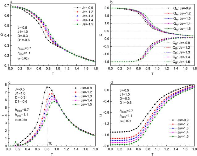
Figure 3. Temperature dependence of (a) the total dynamic order parameter Q, (b) dynamic order parameters QA and QB, (c) susceptibility χ, and (d) the internal energy U for various Js with J = −0.5, J1 = 1.0, D = −0.3, D1 = −0.6, hbias = 0.7, hosc = 1.1 and ω = 0.02π. |
In figure 4, we show Q, QA, QB, χ, and U as functions of temperature for different values of D1 with the fixed values J = −1.6, Js = −1.2, J1 = 1.0, hbias = 0.7, hosc = 1.1, D = −0.3, and ω=0.02π. Two saturation values (Q = 11/16 and 13/16) appear on the Q curves, as shown in figure 4(a). In addition, Q decreases from the saturation value as the temperature increases with the increase in T and eventually approaches a non-zero value because of the magnetic field used as an external bias. In figure 4(b), two saturation values are observed: QB = −3/2 and −7/6. However, QA has a common saturation value QA of 2.0. Furthermore, QA and QB together saturate the Q in figure 4(a), i.e. Q = [(2 × 30) + ((−3/2) × 18)]/48 = 11/16, Q = [(2 × 30) + ((−7/6) × 18)]/48 = 13/16 using equation (5 ). From figure 4(c), we observe that with an increase in ∣D1∣, the corresponding Tb decreases. This is because strong anisotropy changes the system from a high-spin state to a low-spin state. Therefore, with an increase in ∣D1∣, less heat energy is required to break the magnetic order. As shown in figure 4(d), with an increase in ∣D1∣, the U of the system increases. In the low- and high-temperature regions, the value of U increases slowly and rapidly, respectively. This is because each lattice is significantly affected by anisotropy at low temperatures, but the thermal disturbance energy gradually becomes dominant with an increase in temperature. In addition, when the temperature is fixed, the larger the ∣D1∣, the larger the U of the system.
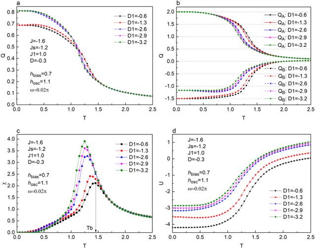
Figure 4. Temperature dependence of (a) the total dynamic order parameter Q, (b) dynamic order parameters QA and QB, (c) susceptibility χ, and (d) the internal energy U for various D1 with J = −1.6, Js = −1.2, J1 = 1.0, D = −0.3, hbias = 0.7, hosc = 1.1, and ω = 0.02π. |
Figure 5 clearly shows the effect of anisotropy D on Q, χ, and U for J = −1.6, Js = −1.2, hbias = 0.7, hosc = 1.1, D1 = −0.6, and ω = 0.02π. In figure 5(a), four saturation values of Q, i.e. 11/16, 7/16, −11/20, and −3/16, at T = 0 are displayed at D = −0.3, −1.3, −2.4, and −3.6, respectively. For instance, when D = −0.3, figure 5(b) shows that the saturation values of the two sublattices are QA = 2.0 and QB = −1.5, respectively. Therefore, the saturation value of the system is Qs = 11/16. When ∣D∣ increases to 1.3, QA decreases and QB remains unchanged. A strong anisotropy can maintain the spin of sublattice A at a low state. Figures 5(c) and (d) show the dynamic order parameters of the five sublattices when D = −2.4 and −3.6, respectively. At T = 0, Q2 = Q4 = Q5 = −1.5 and Q3 = 1.0. However, as D decreases from −2.4 to −3.6, the saturation value of Q1 changes, i.e. Q1 = 13/25 at D = −2.4 and Q1 = 0 at D = −3.6. A more interesting phenomenon is observed when ∣D∣ = 3.6; the Q2, Q3, Q4, Q5 curves of the sublattices change to the opposite direction with increasing T. Notably, when D = −2.4, the saturation value of 13/25 for Q1 is owing to the sublattices not responding to the magnetic field simultaneously, causing the change in direction. The directions of the Q curves labeled −2.4 and −3.6 in figure 5(a) change from negative to positive at a certain T. When the magnetization is zero, the corresponding temperature is called the compensation temperature Tcom, which decreases with increasing ∣D∣. As shown in figure 5(e), Tb increases as ∣D∣ decreases. In addition, double peaks are observed on the χ curve owing to thermal agitation. From figure 5(f), as both T and ∣D∣ increase, U increases. In addition, in the low-temperature zone, a noticeable fluctuation is observed for D = −3.6, where U decreases and then increases. This behavior is related to the changing directions of the Q curves.
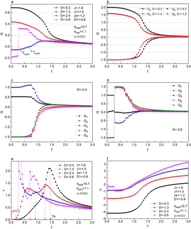
Figure 5. Temperature dependence of (a) the total dynamic order parameter Q, (b) dynamic order parameters QA and QB at D = −0.3 and D = −1.3, (c) dynamic order parameters of the five sublattices at D = −2.4, (d) dynamic order parameter of the five sublattices at D = −3.6, (e) susceptibility χ, and (f) internal energy U for various D with J = −1.6, Js = −1.2, J1 = 1.0, D1 = −0.6, hbias = 0.7, hosc = 1.1, and ω = 0.02π. |
The temperature dependencies of Q, QA, QB, χ, and U for different values of hbias at J = −1.6, Js = −1.2, J1 = 1.0, D = −0.3, D1 = −0.6, hosc = 1.1, and ω = 0.02π, are shown in figure 6. As shown in figure 6(a), all Q curves have the same saturation value (Qs =11/16). When hbias is relatively small (hbias = 0.7, 1.2, or 1.5), the Q curves decrease monotonously with increasing T. When hbias is large (hbias = 1.8, or 2.1), the Q curves first increase and then decrease with an increase in T. We observed that the Q −T curves do not converge to the same value; a high hbias leads to a high convergence value of Q. This reveals that the bias field has a significant impact on the dynamic order parameters at high temperatures. In figure 6(b), the saturation values of QA and QB are observed to be 2.0 and −1.5, respectively. When T < 1.0, the bias field hbias has little effect on QA and QB. However, when T > 1.0, with the increase in hbias, the values of QA and QB decrease significantly. Figure 6(c) shows that Tb increases as hbias increases. This is because an increase in hbias indicates that the magnetic ordering energy of the system increases. Therefore, breaking the order of the system requires more thermal energy to achieve a dynamic paramagnetic phase. In figure 6(d), U is observed to increase with an increase in T but decreases with an increase in the bias field hbias.
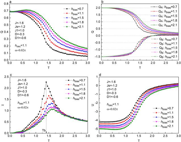
Figure 6. Temperature dependence of (a) the total dynamic order parameter Q, (b) dynamic order parameters QA and QB, (c) susceptibility χ, and (d) internal energy U for different hbias at J = −1.6, Js = −1.2, J1 = 1.0, D = −0.3, D1 = −0.6, hosc = 1.1, and ω = 0.02π. |
Figure 7 shows the effect of hosc on Q, QA, QB, χ, and U at J = −1.6, Js = −1.2, J1 = 1.0, D = −0.3, D1 = −0.6, hbias = 1.5, and ω = 0.02π. As seen in figure 7(a), all Q curves have the same saturation value (Qs =11/16). In the low- (0 < T < 0.75) and high-temperature (1.75 < T < 2.5) regions, Q is not sensitive to T, whereas in the medium-temperature region (0.75 ≤ T ≤ 1.75), T becomes the dominant factor affecting Q. We observe that for the same T, the value of Q decreases as hosc increases. As shown in figure 7(b), when the value of hosc increases, the values of QA and QB gradually decrease. Figure 7(c) reveals that as hosc increases, Tb shifts towards the low-temperature region. The reason for this phenomenon is that when the other parameters are constant, increasing the amplitude of the external magnetic field that is oscillating is equivalent to increasing the disordered energy of the system; thereby reducing the energy required for the system to break the ordered state of the system. Figure 7(d) shows that in the high-temperature region, T, instead of hosc, dominates the influence of internal energy.
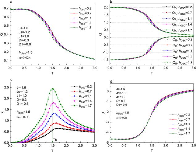
Figure 7. Temperature dependence of (a) the total dynamic order parameter Q, (b) dynamic order parameters QA and QB, (c) susceptibility χ, and (d) internal energy U for various hosc at J = −1.6, Js = −1.2, J1 = 1.0, D = −0.3, D1 = −0.6, hbias = 1.5, and ω = 0.02π. |
The effect of ω on Q, QA, QB, χ, and U at J = −1.3, Js = −1.2, D = −0.3, D1 = −0.6, hbias = 0.7, and hosc = 1.1 is shown in figure 8. In figure 8(a), unlike the other Q-curves (for example, those in figure 2(a)), when T < 1.0 or T > 1.5, Q is insensitive to the changes in ω. When 1.0 ≤ T ≤ 1.5, the value of Q increases as ω increases. This is because, in the case of low or high temperatures, the influence of temperature on the total dynamic order parameters is the main factor. Figure 8(b) shows that both QA and ∣QB∣ decrease as ω decreases and as the temperature increases. Notably, in figure 8(c), Tb increases with the increase in ω; ω represents the frequency of the magnetic field oscillation. When ω is small, the magnetic field oscillates slowly and the spin directions of the sublattices can easily follow the change in the time-dependent oscillating magnetic field, which indicates that the system requires less thermal energy to become disordered. The increased ω causes the dynamic order parameter to not respond instantaneously to the oscillating magnetic field, thereby requiring more thermal energy for phase transition. In figure 8(d), we identify that when T is fixed, U increases as ω increases after local amplification. For the same ω, the value of U increases at high values of T.
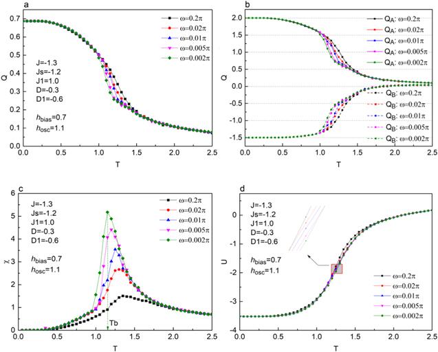
Figure 8. Temperature dependence of (a) the total dynamic order parameter Q, (b) dynamic order parameters QA and QB, (c) susceptibility χ, and (d) internal energy U for different ω at J = −1.3, Js = −1.2, J1 = 1.0, D = −0.3, D1 = −0.6, hbias = 0.7, hosc = 1.1. |
3.2. Phase diagram
To further clarify the effect of various parameters on the blocking temperature, we sorted the results of Tb under the influence of different parameters and plotted the corresponding phase diagrams in figures 9(a)–(f). Figures 9(a)–(b) show the effects of J and Js on Tb with the other parameters set as hbias = 0.7, hosc = 1.1, D = −0.3, D1 = −0.6, and ω = 0.02π. Additionally, Tb increases monotonically with increasing ∣J∣ and ∣Js∣. This is owing to the increase in exchange coupling that essentially increases the interaction forces of the magnetic sublattices in the system, thereby increasing the ordering energy of the system. Therefore, a large Tb is required for the phase transition of the system. In addition, the change in Js has a smaller effect on Tb compared with that of J, because J controls more of the sublattices than Js. Figures 9(c)–(d) show the effect of D and D1 on Tb with other parameters fixed at J = −1.6, Js = −1.2, J1 = 1.0, hbias = 0.7, hosc = 1.1, and ω = 0.02π. Additionally, as D and ∣D1∣ increase, Tb decreases, which indicates that a large anisotropy is not conducive to the order of the system. Moreover, the change in D1 affects Tb less than the changes in D, owing to the reduced number of sublattices with anisotropy D1. Figures 9(e)–(f) show the effect of hbias and hosc on Tb with other parameters fixed at J = −1.6, Js = −1.2, J1 = 1.0, D = −0.3, D1 = −0.6, and ω = 0.02π. Furthermore, Tb increases monotonically with increasing hbias because hbias improves the order of the system. In addition, hbias and hosc have opposite effects on Tb because the increase in hosc increases the disorder of the system.
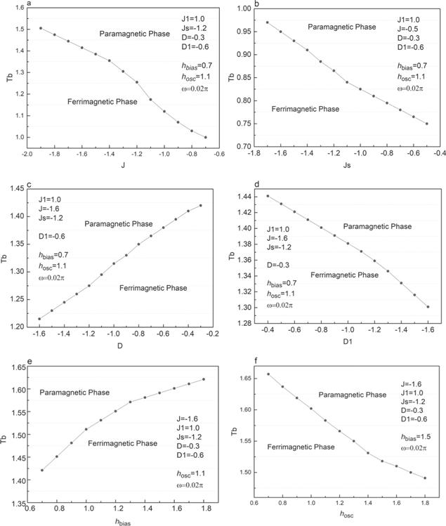
Figure 9. Phase diagrams of Tb (a) in the (J, T) plane with hbias = 0.7, hosc = 1.1, Js = −1.2, D = −0.3, D1 = −0.6, and ω = 0.02π; (b) (Js, T) plane hbias = 0.7, hosc = 1.1, J = −0.5, D = −0.3, D1 = −0.6, and ω = 0.02π; (c) (D, T) plane with J = −1.6, Js = −1.2, D1 = −0.6, hbias = 0.7, hosc = 1.1, and ω = 0.02π; (d) (D1, T) plane with J = −1.6, Js = −1.2, D = −0.3, hbias = 0.7, hosc = 1.1, and ω = 0.02π; (e) (hbias, T) plane J = −1.6, Js = −1.2, D = −0.3, D1 = −0.6, hosc = 1.1, and ω = 0.02π; (f) (hosc, T) plane with J = −1.6, Js = −1.2, D = −0.3, D1 = −0.6, hbias = 1.5, and ω = 0.02π. |
3.3. Magnetocaloric effect
The magnetocaloric effect on the Kagome lattice was investigated. The temperature dependence of magnetization M of the Kagome lattice is shown in figure 10. We observe that M starts at the saturation value (Ms = 29/16) at zero temperature and then decreases with increasing T. Figure 11 shows the thermal magnetizations (dM/dT) with different values of bias field hbias. These curves indicate that at the critical temperature Tc, the magnetic transition changes from the ferromagnetic phase to the paramagnetic phase. The corresponding transition temperatures increase with increasing hbias. For example, Tc = 1.601 for hbias = 1.0 and Tc = 2.101 for hbias = 5.0. We calculated the magnetic entropy using equation (11 ). Figure 12 shows the variation trend in the magnetic entropy ΔS of the Kagome lattice as a function of T with different hbias. A maximum value at the critical temperature can be seen in the −ΔS curves. This maximum value $-{\rm{\Delta }}{S}_{\max }$ increases with increasing hbias. For hbias = 1.0, 2.0, 3.0, 4.0, and 5.0, $-{\rm{\Delta }}{S}_{\max }$ = 1.759, 2.639, 3.295, 3.880, and 4.426, respectively. In addition, figure 13 shows an interesting parameter for evaluating potential materials for magnetic refrigeration, i.e. RCP, which is a function of hbias for the Kagome lattice. Furthermore, RCP is found to increase linearly as hbias increases and reaches a value of 8.281 at hbias = 6.0.
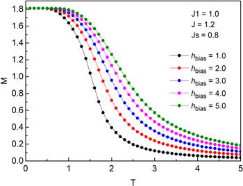
Figure 10. Magnetization as a function of T for different hbias. |
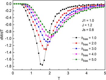
Figure 11. dM/dT as a function of T for different hbias. |
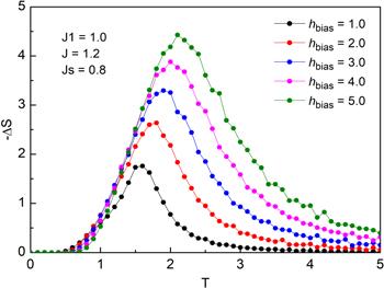
Figure 12. Temperature dependence of the entropy variation with different hbias. |
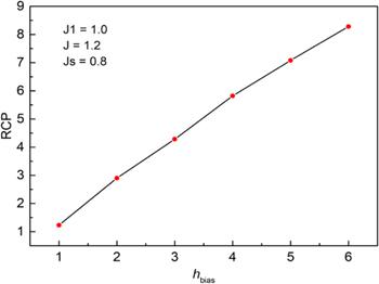
Figure 13. Bias field dependence of the RCP associated with the system for J1 = 1.0, J = 1.2, and Js = 0.8. |
Figure 14 shows the dependence of T on the M of the system. The figure shows that all M curves decrease from the saturation value (Ms = 29/16) to a steady-state value with increasing T. When T is fixed, M increases with increasing J. Figure 15 shows the (dM/dT) curves for different values of J. At Tc, the magnetic transition changes from the ferromagnetic phase to the paramagnetic phase. Furthermore, Tc increases with increasing J, i.e. Tc = 1.801 for J = 0.8 and Tc = 2.401 for J = 2.4. Figure 16 shows the variation of −ΔS with the changes in temperature of the Kagome lattice for different values of J. The −ΔS curves reach a maximum value $-{\rm{\Delta }}{S}_{\max }$ at Tc. This maximum value decreases with increasing J, i.e. for J =0.8, 1.2, 1.6, 2.0, and 2.4, $-{\rm{\Delta }}{S}_{\max }$ = 3.384, 3.323, 3.169, 3.083, and 2.966, respectively. Figure 17 shows J dependence of the RCP associated with the system. We found that RCP decreases linearly with increasing J.
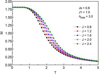
Figure 14. Magnetization as a function of T for different hbias. |
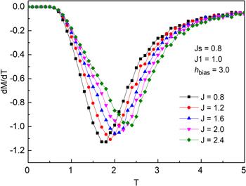
Figure 15. dM/dT as a function of T for different J. |

Figure 16. Temperature dependence of the entropy variation with different J. |
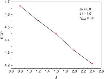
Figure 17. Exchange-coupling J dependence of the RCP associated with the system at hbias = 3.0, Js = 0.8, and J1 = 1.0. |
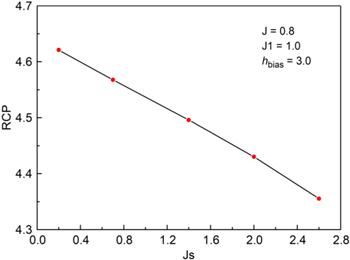
Figure 18 shows the M versus T plots for different values of Js at J = 1.2, J1 = 1.0, and hbias = 3.0. Only one saturation value (Ms = 29/16) is shown in the figure. In figures 19 and 20, we additionally show (dM/dT) and −ΔS as a function of temperature with the same parameters as those in figure 19. The peaks corresponding to the Tc of the system increase with increasing Js. Figure 21 shows the exchange-coupling Js dependence of the RCP associated with the system. The RCP decreases with increasing Js, similar to that in figure 17.
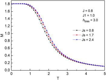
Figure 18. Magnetization as a function of T for different Js. |
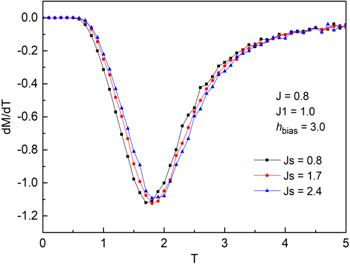
Figure 19. dM/dT as a function of T for different Js. |
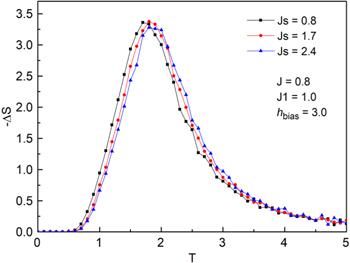
Figure 20. Temperature dependence of the entropy variation with different Js. |
Figure 21. Exchange-coupling Js dependence of the RCP associated with the system at hbias = 3.0, J = 1.2, and J1 = 1.0. |
4. Conclusions
In this study, we investigated the ferrimagnetic mixed-spin (2, 3/2) Kagome lattice using MC simulations. We discuss the effect of J, Js, D, D1, hbias, hosc, and ω on the dynamic phase transitions of the system. The system exhibits multiple spin flips when the system parameters are changed, and under certain parametric conditions, compensation point behavior is exhibited by the system. By analyzing the phase diagrams of Tb, we found that large ∣J∣, ∣Js∣, hbias, and ω values facilitate an increase in Tb; however, the increases in D, D1, and hosc have the opposite effect on Tb. Moreover, ΔS as a function of T for various hbias (J and Js) were also discussed. The RCP revealed that the magnetocaloric effect depends on the values of hbias, J and Js.