


1. Introduction
The exact solutions of nonlinear equations are very important in many fields. Soliton solutions, lump solutions, breather solutions, and interaction solutions can completely describe nonlinear phenomena in nature. One special kind of rational solution is the lump solution. It has spatial localization and shape invariance. Satsuma and Ablowitz [1] obtained the lump solutions in their research of the Kadomtsev–Petviashvili equation by taking the long-wave limit for the N-soliton solutions. Since then, the long-wave limit method has been widely used to discover the lump solutions of various nonlinear equations. In 2015, Ma [2] presented the positive quadratic function method, which was adopted by numerous scholars to obtain lump solutions [3–5]. There is a solution with periodic oscillations and localization, similar to breathing, hence the name of the breather solution. It is divided into three categories: Kuznetsov–Ma breather, Akhmediev breather, and general breather [6–8]. We can derive the breather solutions by treating the parameters of N-soliton solutions as conjugate relations, and this method is known as the complex conjugate method. In recent years, lump solutions, breather solutions, and hybrid solutions have been studied, such as (2+1)-dimensional extended shallow water wave equation [9], (2+1)-dimensional Hirota–Satsuma–Ito equation [10], (2+1)-dimensional Sawada–Kotera equation [11, 12], the combined pKP-BKP equation [13], potential Kadomtsev–Petviashvili equation [14], (2+1)-dimensional asymmetrical Nizhnik–Novikov–Veselov equation [15, 16], (2+1)-dimensional Bogoyavlenskii–Schieff equation [17], and so on [18–26].
The (2+1)-dimensional Boiti–Leon–Manna–Pempinelli (BLMP) equation
$\begin{eqnarray}{v}_{{yt}}+{v}_{{xxxy}}-3{v}_{x}{v}_{{xy}}-3{v}_{{xx}}{v}_{y}=0,\end{eqnarray}$
which was developed by Gilson et al [27]. BLMP equation has been an important model in incompressible fluid [28]. In recent years, numerous results of this equation have been investigated by experts. Using the Bäcklund transformation generated by the modified Clarkson–Kruskal direct technique, Li et al [29] found new solutions to the equation and explained the connection between the new and old solutions. The start and step solutions for the (2+1) and (3+1)-dimensional equations were obtained by Darvishi et al [30] using the multi-exponential function method. Then the extended homoclinic test approach was used by Tang et al [31] to study the exact solutions of these two equations. Kaplan et al [32] used the homogeneous balance method to build the Auto-Bäcklund transformation of the equation. Hu et al [33, 34] used the Pfaffian technique and the optimized Pfaffian technique to study the solutions, respectively.Guo et al [35] modified the above equation and obtained the (2+1)-dimensional extended BLMP (eBLMP) equation2 ) extends BLMP equation (1 ) by introducing two second-order derivatives uyy and uxx, which change the dispersion relations of the original equation. Due to the arbitrariness of δ1 and δ2, equation (2 ) can explain more dispersion relations and enrich their applications in reality. In [35], the experts used the positive quadratic method to obtain the lump and lump-kink soliton solutions. Then Shen et al [36] applied the extended homogeneous test, Riemann theta function, and polynomial expansion approach to obtain the breather solutions, periodic-wave solutions, and traveling-wave solutions, respectively. To our knowledge, no literature has investigated the exact solutions of the (2+1)-dimensional eBLMP equation by using the long-wave limit approach and the conjugate complex method. These two methods will be used to obtain the M-lump solutions, T-order breather solutions, and the interaction solutions with solitons in this paper.
$\begin{eqnarray}\begin{array}{l}{u}_{{yt}}+{u}_{{xxxy}}+3{u}_{x}{u}_{{xy}}+3{u}_{y}{u}_{{xx}}\\ \quad +{\delta }_{1}{u}_{{yy}}+{\delta }_{2}{u}_{{xx}}=0,\end{array}\end{eqnarray}$
where δ1 and δ2 are arbitrary constants. Equation (Following is a framework for this paper. The bilinear method is used in the second section to derive both the bilinear form and the N-soliton solution of the equation. In section 3 , the 1-, 2-, and 3-lump solutions as well as the M-lump expressions are discovered utilizing the long-wave limit method. In section 4 , we discover the interactions between lump solutions and soliton solutions. In section 5 , we demonstrate how to use the conjugate relations to convert N-soliton solutions to T-order breather solutions. For T = 1, 2, and 3, specific breather solutions are also presented. The breather solution's interactions with the soliton solutions and lump solutions are shown in section 6 and 7 , respectively. Using the mathematical software Maple, we draw the 3D and density plots related to each solution to observe their dynamic characteristics. Then the paper ends with a summary.
2. N-soliton solutions
First, we consider the variable transformation2 ) then, as4 ) under the variable transformation (3 ), we can discover the relationship: u(x, y, t) is an answer to equation (2 ). The N-soliton solutions of equation (4 ) can be derived by applying the Hirota bilinear method. And fN will be expressed as6 ), ∑μ=0,1 denotes the sum of all combinations of μi = 0, 1(1 ≤ i ≤ N). The symbol ${\sum }_{i\lt j}^{N}$ means the sum of all combinations of pairs (i, j) chosen from the set {1, 2, …, N} with the condition i < j.
$\begin{eqnarray}u(x,y,t)=2{\left(\mathrm{ln}f\right)}_{x}.\end{eqnarray}$
It is straightforward to calculate the bilinear form of the equation ( $\begin{eqnarray}\begin{array}{l}{BF}=({D}_{y}{D}_{t}+{D}_{x}^{3}{D}_{y}+{\delta }_{1}{D}_{y}^{2}+{\delta }_{2}{D}_{x}^{2})f\cdot f\\ \quad ={f}_{{yt}}f-{f}_{y}{f}_{t}+{f}_{{xxxy}}f-{f}_{{xxx}}{f}_{y}+3{f}_{{xx}}{f}_{{xy}}\\ \quad -3{f}_{x}{f}_{{xxy}}+{\delta }_{1}({f}_{{yy}}f-{f}_{y}^{2})\\ \quad +{\delta }_{2}({f}_{{xx}}f-{f}_{x}^{2})=0,\end{array}\end{eqnarray}$
where f = f(x, y, t), and the bilinear operators Dx, Dy, and Dt are defined by $\begin{eqnarray}\begin{array}{l}{D}_{x}^{m}{D}_{y}^{n}{D}_{t}^{s}(f\cdot {f}_{1})\\ \quad ={\left(\displaystyle \frac{\partial }{\partial x}-\displaystyle \frac{\partial }{\partial {x}_{1}}\right)}^{m}{\left(\displaystyle \frac{\partial }{\partial y}-\displaystyle \frac{\partial }{\partial {y}_{1}}\right)}^{n}{\left(\displaystyle \frac{\partial }{\partial t}-\displaystyle \frac{\partial }{\partial {t}_{1}}\right)}^{s}\\ \quad \times [f(x,y,t){f}_{1}({x}_{1},{y}_{1},{t}_{1})]{| }_{{x}_{1}=x,{y}_{1}=y,{t}_{1}=t}.\end{array}\end{eqnarray}$
When f is an answer to equation ( $\begin{eqnarray}{f}_{N}=\displaystyle \sum _{\mu =0,1}\exp (\displaystyle \sum _{i=1}^{N}{\mu }_{i}{\chi }_{i}+\displaystyle \sum _{i\lt j}^{N}{\mu }_{i}{\mu }_{j}{{\rm{\Omega }}}_{{ij}}),\end{eqnarray}$
where $\begin{eqnarray}\begin{array}{l}{\chi }_{i}={h}_{i}\left(x+{\rho }_{i}y+{w}_{i}t\right)+{\chi }_{i}^{0},\\ {w}_{i}=-{h}_{i}^{2}-{\delta }_{1}{\rho }_{i}-\displaystyle \frac{{\delta }_{2}}{{\rho }_{i}},\end{array}\end{eqnarray}$
$\begin{eqnarray}{{\rm{e}}}^{{{\rm{\Omega }}}_{{ij}}}=\displaystyle \frac{3{\rho }_{i}{\rho }_{j}({h}_{i}-{h}_{j})({h}_{i}{\rho }_{i}-{h}_{j}{\rho }_{j})-{\delta }_{2}{\left({\rho }_{i}-{\rho }_{j}\right)}^{2}}{3{\rho }_{i}{\rho }_{j}({h}_{i}+{h}_{j})({h}_{i}{\rho }_{i}+{h}_{j}{\rho }_{j})-{\delta }_{2}{\left({\rho }_{i}-{\rho }_{j}\right)}^{2}},\end{eqnarray}$
where hi, ρi, and ${\chi }_{i}^{0}$ are arbitrary parameters. In the expression (3. M-lump solutions
By applying the long-wave limit method on the N-soliton solutions, we can obtain the multi-lump solutions of equation (2 ). First, we take every $\exp ({\chi }_{i}^{0})=-1$, the expression (6 ) can be written as2 ). To simplify the calculation, we eliminate the common factorization ${\prod }_{i=1}^{N}{h}_{i}$. The simplified fN is
$\begin{eqnarray}{f}_{N}=\displaystyle \sum _{\mu =0,1}\displaystyle \prod _{i=1}^{N}{\left(-1\right)}^{{\mu }_{i}}\exp ({\mu }_{i}{\alpha }_{i})\displaystyle \prod _{i\lt j}^{N}\exp ({\mu }_{i}{\mu }_{j}{{\rm{\Omega }}}_{{ij}}),\end{eqnarray}$
where ${\alpha }_{i}={h}_{i}(x+{\rho }_{i}y+(-{h}_{i}^{2}-{\delta }_{1}{\rho }_{i}-\tfrac{{\delta }_{2}}{{\rho }_{i}})t)$. If we take the long-wave limit as hi → 0, we obtain $\begin{eqnarray}\begin{array}{l}{f}_{N}=\displaystyle \sum _{\mu =0,1}\displaystyle \prod _{i=1}^{N}{\left(-1\right)}^{{\mu }_{i}}(1+{\mu }_{i}{h}_{i}{\beta }_{i})\\ \quad \displaystyle \prod _{i\lt j}^{N}(1+{\mu }_{i}{h}_{i}{\mu }_{j}{h}_{j}{Q}_{{ij}})+O({k}^{N+1}),\end{array}\end{eqnarray}$
with $\begin{eqnarray}\begin{array}{l}{\beta }_{i}=x+{\rho }_{i}y+\left(-{\delta }_{1}{\rho }_{i}-\displaystyle \frac{{\delta }_{2}}{{\rho }_{i}}\right)t,{Q}_{{ij}}\\ \quad =\displaystyle \frac{6{\rho }_{i}{\rho }_{j}({\rho }_{i}+{\rho }_{j})}{{\delta }_{2}{\left({\rho }_{i}-{\rho }_{j}\right)}^{2}},(i,j=1,\ldots ,N;i\ne j).\end{array}\end{eqnarray}$
By simplifying fN, the common factorization ${\prod }_{i=1}^{N}{h}_{i}$ can be derived from it. When performing the calculation of $u=2{\left(\mathrm{ln}f\right)}_{x}$, it is found that the presence or absence of the common factorization ${\prod }_{i=1}^{N}{h}_{i}$ does not affect the result of u. Therefore it is easy to prove that $u=2{\left(\mathrm{ln}\tfrac{{f}_{N}}{{\prod }_{i=1}^{N}{h}_{i}}\right)}_{x}$ is also a solution of the equation ( $\begin{eqnarray}\begin{array}{l}{f}_{N}=\displaystyle \prod _{i=1}^{N}{\beta }_{i}+\displaystyle \frac{1}{2}\displaystyle \sum _{i,j}^{N}{Q}_{{ij}}\displaystyle \prod _{r\ne i,j}^{N}{\beta }_{r}\,+\cdots \\ \quad +\displaystyle \frac{1}{M!{2}^{M}}\displaystyle \sum _{i,j,\cdots ,m,n}^{N}\mathop{\overbrace{{Q}_{{ij}}{Q}_{{pq}}\cdots {Q}_{{mn}}}}\limits^{M}\\ \quad \displaystyle \prod _{s\ne i,j,p,q,\cdots ,m,n}^{N}{\beta }_{s}+\cdots .\end{array}\end{eqnarray}$
If we choose the condition $N=2M,{\rho }_{M+i}\,={\rho }_{i}^{* }(i=1,2,\ldots ,M),$ and Qij > 0, where * denotes the complex conjugation, we can get a class of general M-lump solutions. In the following, we list the 1-lump, 2-lump, and 3-lump solutions individually.3.1. 1-lump solutions
With M = 1, N = 2 in equation (12 ), it can be simplified into14 ) into equation (3 ), we can obtain15 ) we obtain is the 1-lump solution of the equation (2 ). And this solution moves along a line $y=\tfrac{\left(\left({a}^{2}+{b}^{2}\right){\delta }_{1}-{\delta }_{2}\right)}{2a{\delta }_{2}}(x-\sqrt{-\tfrac{3a\left({a}^{2}+{b}^{2}\right)}{{\delta }_{2}\cdot {b}^{2}}})$ with the velocity ${v}_{x}=\tfrac{2a{\delta }_{2}}{{a}^{2}+{b}^{2}}$ along the x-axis and ${v}_{y}=\tfrac{(({a}^{2}+{b}^{2}){\delta }_{1}-{\delta }_{2})}{{a}^{2}+{b}^{2}}$ along the y-axis. If we take the parameters as $a=\tfrac{1}{2},b=1,{\delta }_{1}=1,{\delta }_{2}=-1$, the evolution of the 1-lump solution at time t = −10, 0, 10 can be drawn in figure 1. It can be observed from the images that the 1-lump wave maintains the same speed and shape during propagation and travels in the same direction.
$\begin{eqnarray}{f}_{1}={\beta }_{1}{\beta }_{2}+{Q}_{12},\end{eqnarray}$
where β1 = x + ρ1y + $(-{\delta }_{1}{\rho }_{1}-\tfrac{{\delta }_{2}}{{\rho }_{1}})t$, β2 = x + ρ2y + ( − δ1ρ2 − $\tfrac{{\delta }_{2}}{{\rho }_{2}})t$, ${Q}_{12}=\tfrac{6{\rho }_{1}{\rho }_{2}({\rho }_{1}+{\rho }_{2})}{{\delta }_{2}{\left({\rho }_{1}-{\rho }_{2}\right)}^{2}}$ and ${\rho }_{2}={\rho }_{1}^{* }$. If we setup the parameter ρ1 = a + bi, a, b are real constants. The f1 can be written as $\begin{eqnarray}\begin{array}{l}{f}_{1}={\left[x+{ay}-\displaystyle \frac{a(({a}^{2}+{b}^{2}){\delta }_{1}+{\delta }_{2})}{{a}^{2}+{b}^{2}}t\right]}^{2}\\ \quad +{b}^{2}{\left[y-\displaystyle \frac{(({a}^{2}+{b}^{2}){\delta }_{1}-{\delta }_{2})}{{a}^{2}+{b}^{2}}t\right]}^{2}\\ \quad -\displaystyle \frac{3a({a}^{2}+{b}^{2})}{{\delta }_{2}{b}^{2}}\\ \quad ={\left(X+{aY}\right)}^{2}+{b}^{2}{Y}^{2}-\displaystyle \frac{3a({a}^{2}+{b}^{2})}{{\delta }_{2}{b}^{2}},\end{array}\end{eqnarray}$
where $X=x-\tfrac{2a{\delta }_{2}}{{a}^{2}+{b}^{2}}t$ and $Y=y-\tfrac{(({a}^{2}+{b}^{2}){\delta }_{1}-{\delta }_{2})}{{a}^{2}+{b}^{2}}t$. Substituting equation ( $\begin{eqnarray}u=\displaystyle \frac{4(X+{aY})}{{\left(X+{aY}\right)}^{2}+{b}^{2}{Y}^{2}-\tfrac{3a({a}^{2}+{b}^{2})}{{\delta }_{2}{b}^{2}}},\end{eqnarray}$
which satisfies the condition $-\tfrac{a}{{\delta }_{2}}\gt 0$. The equation (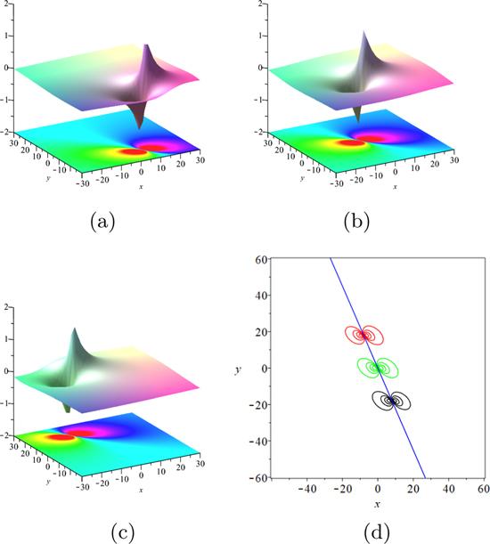
Figure 1. 1-lump solution ( |
3.2. 2-lump solutions
When M = 2, N = 4 in equation (12 ), it is reduced to3 ) with parameters ${\rho }_{3}={\rho }_{1}^{* }$ = a1 − b1i, ${\rho }_{4}={\rho }_{2}^{* }={a}_{2}-{b}_{2}{\rm{i}}$, we will obtain the 2-lump solution of the equation (2 ). By calculation, two lump waves move along straight lines $y=\tfrac{\left(\left({a}_{1}^{2}+{b}_{1}^{2}\right){\delta }_{1}-{\delta }_{2}\right)}{2{a}_{1}{\delta }_{2}}$ $(x-\sqrt{-\tfrac{3{a}_{1}\left({a}_{1}^{2}+{b}_{1}^{2}\right)}{{\delta }_{2}{b}_{1}^{2}}})$ and $y=\tfrac{\left(\left({a}_{2}^{2}+{b}_{2}^{2}\right){\delta }_{1}-{\delta }_{2}\right)}{2{a}_{2}{\delta }_{2}}$ $(x-\sqrt{-\tfrac{3{a}_{2}\left({a}_{2}^{2}+{b}_{2}^{2}\right)}{{\delta }_{2}\cdot {b}_{2}^{2}}})$, respectively. Here, we take the parameters as ${a}_{1}=\tfrac{2}{3}$, b1 = 3, ${a}_{2}=\tfrac{1}{3},{b}_{2}=\tfrac{1}{2}$ and δ1 = 1, δ2 = −1. The evolutions of the 2-lump solution at time t = −15, 0, 15 are shown in figure 2. As shown in the images, the two lump waves move along their respective trajectories. During the time variation from −15 to 15, the two lumps approach gradually, then collide at the moment t = 0, and finally move away from each other and return to their original shapes.
$\begin{eqnarray}\begin{array}{rcl}{f}_{2} & = & {\beta }_{1}{\beta }_{2}{\beta }_{3}{\beta }_{4}+{Q}_{12}{\beta }_{3}{\beta }_{4}+{Q}_{13}{\beta }_{2}{\beta }_{4}\\ & & +{Q}_{14}{\beta }_{2}{\beta }_{3}+{Q}_{23}{\beta }_{1}{\beta }_{4}\\ & & +{Q}_{24}{\beta }_{1}{\beta }_{3}+{Q}_{34}{\beta }_{1}{\beta }_{2}+{Q}_{12}{Q}_{34}\\ & & +{Q}_{13}{Q}_{24}+{Q}_{14}{B}_{23},\end{array}\end{eqnarray}$
where βi = x + ρiy + ( −δ1ρi − $\tfrac{{\delta }_{2}}{{\rho }_{i}})t$, ${Q}_{{ij}}=\tfrac{6{\rho }_{i}{\rho }_{j}({\rho }_{i}+{\rho }_{j})}{{\delta }_{2}{\left({\rho }_{i}-{\rho }_{j}\right)}^{2}}$, 1 ≤ i < j ≤ 4. Bringing f2 into the equation (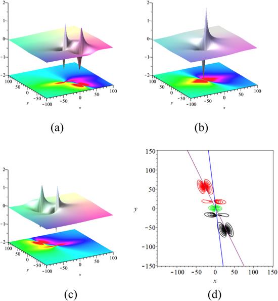
Figure 2. 2-lump solution with ${\rho }_{3}={\rho }_{1}^{* }=\tfrac{2}{3}-3{\rm{i}},{\rho }_{4}={\rho }_{2}^{* }=\tfrac{1}{3}-\tfrac{1}{2}{\rm{i}}$, δ1 = 1, δ2 = −1, at (a) t = −15; (b) t = 0; (c) t = 15; (d) shows two lump waves travel along the lines $y=-\tfrac{49}{24}(x-\tfrac{\sqrt{13}}{3})$ (purple) and $y=-\tfrac{47}{6}(x-\tfrac{\sqrt{170}}{9})$ (blue). |
3.3. 3-lump solutions
Similarly, let M = 3, N = 6 in the equation (12 ), we can obtain the function f3 with 76 terms, where ${\beta }_{i}=x+{\rho }_{i}y+(-{\delta }_{1}{\rho }_{i}-\tfrac{{\delta }_{2}}{{\rho }_{i}})t,{Q}_{{ij}}=\tfrac{6{\rho }_{i}{\rho }_{j}({\rho }_{i}+{\rho }_{j})}{{\delta }_{2}{\left({\rho }_{i}-{\rho }_{j}\right)}^{2}},1\leqslant {\rm{i}}\lt j\leqslant 6$. And we can derive the expression of 3-lump solution u after bringing f3 into variable transformation equation (3 ). Letting ${\rho }_{4}={\rho }_{1}^{* }$ = a1 − b1i, ${\rho }_{5}={\rho }_{2}^{* }$ = a2 − b2i, ${\rho }_{6}={\rho }_{3}^{* }$ = a3 − b3i, 3-lump solution is obtained (see figure 3). By calculation, three lump waves move along three straight lines $y=\tfrac{\left(\left({a}_{1}^{2}+{b}_{1}^{2}\right){\delta }_{1}-{\delta }_{2}\right)}{2{a}_{1}{\delta }_{2}}$ $(x-\sqrt{-\tfrac{3{a}_{1}\left({a}_{1}^{2}+{b}_{1}^{2}\right)}{{\delta }_{2}{b}_{1}^{2}}})$, $y=\tfrac{\left(\left({a}_{2}^{2}+{b}_{2}^{2}\right){\delta }_{1}-{\delta }_{2}\right)}{2{a}_{2}{\delta }_{2}}$ $(x-\sqrt{-\tfrac{3{a}_{2}\left({a}_{2}^{2}+{b}_{2}^{2}\right)}{{\delta }_{2}\cdot {b}_{2}^{2}}})$, and $y=\tfrac{\left(\left({a}_{3}^{2}+{b}_{3}^{2}\right){\delta }_{1}-{\delta }_{2}\right)}{2{a}_{3}{\delta }_{2}}$ $(x-\sqrt{-\tfrac{3{a}_{3}\left({a}_{3}^{2}+{b}_{3}^{2}\right)}{{\delta }_{2}\cdot {b}_{3}^{2}}})$, respectively, which can be seen in figure 3(d). The evolutions of the 3-lump solution at time t = −20, 0, 20 are shown in figures 3(a)–(c). Similarly, the three waves will collide and change their shapes during moving. However, it has the same shape after the collision as before.

Figure 3. 3-lump solution with ${\rho }_{4}={\rho }_{1}^{* }=\tfrac{2}{3}-\tfrac{1}{2}{\rm{i}},{\rho }_{5}={\rho }_{2}^{* }=\tfrac{1}{3}-\tfrac{1}{2}{\rm{i}},{\rho }_{6}={\rho }_{3}^{* }=\tfrac{2}{3}-{\rm{i}}$, δ1 = 1, δ2 = −1, at (a) t = −20; (b) t = 0; (c) t = 20; (d) shows three lump waves travel along the line $y=-\tfrac{49}{24}(x-\tfrac{\sqrt{13}}{3})$ (black), $y=-\tfrac{11}{6}(x-\tfrac{\sqrt{26}}{3})$ (orange), and $y=-\tfrac{61}{48}(x-\tfrac{5\sqrt{2}}{3})$ (blue–green). |
4. Hybrid solutions between lumps and solitons
In the previous section, we study the M-lump solution. And in this section, we will further investigate the interaction of lump waves with soliton waves. The method used is also the long-wave limit method. These hybrid solutions are derived from the expression (6 ) by taking the parameters
$\begin{eqnarray}\begin{array}{l}N=2M+K,{\chi }_{1}^{0}={\chi }_{2}^{0}=\cdots ={\chi }_{2M}^{0}={\rm{i}}\pi ,\\ \quad {h}_{1},\ldots ,{h}_{2M}\to 0,{\rho }_{r+M}={\rho }_{r}^{* }\\ \quad ={a}_{r}-{b}_{r}{\rm{i}},(r=1,2,\ldots ,M),\end{array}\end{eqnarray}$
where M and K are the positive integers, ar, br, hs, ρs and ${\chi }_{s}^{0}$ are the real constants (s = 2M + 1, …2M + K).4.1. A hybrid solution between 1-lump and 1-soliton
For instance, in order to study the interaction solution of 1-lump and 1-soliton, we need to take the parameters as6 ), we have19 ). The evolutions of the hybrid solution at time t = −10, 0, 10 are shown in figure 4. In these pictures, we find that the lump wave and soliton wave are moving in opposite directions. From −10 to 0 min, they gradually approach and collide at t = 0 (figure 4b). The shapes of both waves are changed by the collision and the waves move independently after separation.
$\begin{eqnarray}\begin{array}{l}N=3,M=1,K=1,{\chi }_{1}^{0}={\chi }_{2}^{0}={\rm{i}}\pi ,\\ {h}_{1},{h}_{2}\to 0,{\rho }_{2}={\rho }_{1}^{* }={a}_{1}-{b}_{1}{\rm{i}}.\end{array}\end{eqnarray}$
Then bring them into equation ( $\begin{eqnarray}\begin{array}{l}{f}_{\mathrm{1,1}}={\beta }_{1}{\beta }_{2}+{Q}_{12}+({Q}_{13}{Q}_{23}+{Q}_{13}{\beta }_{2}\\ \quad +{Q}_{23}{\beta }_{1}+{Q}_{12}+{\beta }_{1}{\beta }_{2})\cdot {{\rm{e}}}^{{\chi }_{3}},\end{array}\end{eqnarray}$
with $\begin{eqnarray}\begin{array}{rcl}{\beta }_{i} & = & x+{\rho }_{i}y+(-{\delta }_{1}{\rho }_{i}-\displaystyle \frac{{\delta }_{2}}{{\rho }_{i}})t,(i=1,2),\\ {\chi }_{3} & = & {h}_{3}\left(x+{\rho }_{3}y+(-{h}_{3}^{2}-{\delta }_{1}{\rho }_{3}-\displaystyle \frac{{\delta }_{2}}{{\rho }_{3}})t\right)+{\chi }_{3}^{0},\\ {Q}_{12} & = & \displaystyle \frac{6{\rho }_{1}{\rho }_{2}({\rho }_{1}+{\rho }_{2})}{{\delta }_{2}{\left({\rho }_{1}-{\rho }_{2}\right)}^{2}},{Q}_{13}=-\displaystyle \frac{6{\rho }_{1}{\rho }_{3}({\rho }_{1}+{\rho }_{3})}{3{\rho }_{1}{\rho }_{3}^{2}{h}_{3}^{2}-{\delta }_{2}{\left({\rho }_{1}-{\rho }_{3}\right)}^{2}},\\ {Q}_{23} & = & -\displaystyle \frac{6{\rho }_{2}{\rho }_{3}({\rho }_{2}+{\rho }_{3})}{3{\rho }_{2}{\rho }_{3}^{2}{h}_{3}^{2}-{\delta }_{2}{\left({\rho }_{2}-{\rho }_{3}\right)}^{2}}.\end{array}\end{eqnarray}$
The hybrid solution between 1-lump and 1-soliton can be gained after calculating $u=2{\left(\mathrm{ln}{f}_{\mathrm{1,1}}\right)}_{x}$ and choosing ${a}_{1}=\tfrac{1}{2},{b}_{1}=1,{h}_{3}=1,{\rho }_{3}=-\tfrac{1}{2},{\chi }_{3}^{0}=0$. δ1 = 1, δ2 = −1, where f1,1 is given by (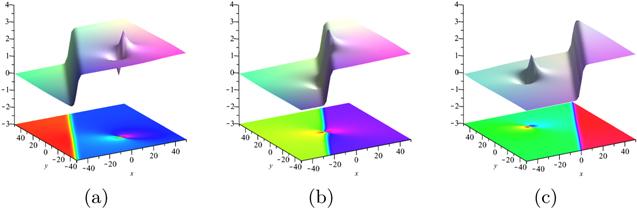
Figure 4. Hybrid solution between 1-lump and 1-soliton with ${\rho }_{2}={\rho }_{1}^{* }$ = $\tfrac{1}{2}-{\rm{i}}$, h3 = 1, ${\rho }_{3}=-\tfrac{1}{2}$, ${\chi }_{3}^{0}=0$, δ1 = 1, δ2 = −1, at (a) t = −10; (b) t = 0; (c) t = 10. |
4.2. A hybrid solution between 1-lump and 2-solitons
Similarly, to find the interaction solution of 1-lump and 2-solitons, we take6 ), we have
$\begin{eqnarray}\begin{array}{l}N=4,M=1,K=2,{\chi }_{1}^{0}={\chi }_{2}^{0}={\rm{i}}\pi ,\\ {h}_{1},{h}_{2}\to 0,{\rho }_{2}={\rho }_{1}^{* }={a}_{1}-{b}_{1}{\rm{i}}.\end{array}\end{eqnarray}$
Then bring them into equation ( $\begin{eqnarray}\begin{array}{l}{f}_{\mathrm{1,2}}={\beta }_{1}{\beta }_{2}+{Q}_{12}+({\beta }_{1}{\beta }_{2}+{Q}_{23}{\beta }_{1}\\ \quad +{Q}_{13}{\beta }_{2}+{Q}_{13}{Q}_{23}+{Q}_{12})\cdot {{\rm{e}}}^{{\chi }_{3}}\\ \quad +({\beta }_{1}{\beta }_{2}+{Q}_{24}{\beta }_{1}+{Q}_{14}{\beta }_{2}+{Q}_{14}{Q}_{24}+{Q}_{12})\cdot {{\rm{e}}}^{{\chi }_{4}}\\ \quad +\left[{\beta }_{1}{\beta }_{2}+({Q}_{23}+{Q}_{24}){\beta }_{1}+({Q}_{13}+{Q}_{14}){\beta }_{2}\right.\\ \quad +{Q}_{12}+{Q}_{13}{Q}_{23}\\ \quad \left.+{Q}_{14}{Q}_{23}+{Q}_{13}{Q}_{24}+{Q}_{14}{Q}_{24}\right]\cdot {{\rm{e}}}^{{\chi }_{3}+{\chi }_{4}+{{\rm{\Omega }}}_{34}},\end{array}\end{eqnarray}$
with $\begin{eqnarray}\begin{array}{l}{\beta }_{1}=x+{\rho }_{1}y+\left(-{\delta }_{1}{\rho }_{1}-\frac{{\delta }_{2}}{{\rho }_{1}}\right)t,\\ {\beta }_{2}=x+{\rho }_{2}y+\left(-{\delta }_{1}{\rho }_{2}-\frac{{\delta }_{2}}{{\rho }_{2}}\right)t,\\ {\chi }_{3}={h}_{3}\left(x+{\rho }_{3}y+(-{h}_{3}^{2}-{\delta }_{1}{\rho }_{3}-\frac{{\delta }_{2}}{{\rho }_{3}})t\right)+{\chi }_{3}^{0},\\ {\chi }_{4}={h}_{4}\left(x+{\rho }_{4}y+(-{h}_{4}^{2}-{\delta }_{1}{\rho }_{4}-\frac{{\delta }_{2}}{{\rho }_{4}})t\right)+{\chi }_{4}^{0},\\ {Q}_{12}=\frac{6{\rho }_{1}{\rho }_{2}({\rho }_{1}+{\rho }_{2})}{{\delta }_{2}{\left({\rho }_{1}-{\rho }_{2}\right)}^{2}},{Q}_{13}=-\frac{6{\rho }_{1}{\rho }_{3}({\rho }_{1}+{\rho }_{3})}{3{\rho }_{1}{\rho }_{3}^{2}{h}_{3}^{2}-{\delta }_{2}{\left({\rho }_{1}-{\rho }_{3}\right)}^{2}},\\ {Q}_{23}=-\frac{6{\rho }_{2}{\rho }_{3}({\rho }_{2}+{\rho }_{3})}{3{\rho }_{2}{\rho }_{3}^{2}{h}_{3}^{2}-{\delta }_{2}{\left({\rho }_{2}-{\rho }_{3}\right)}^{2}},\\ {Q}_{14}=\frac{-6{\rho }_{1}{\rho }_{4}({\rho }_{1}+{\rho }_{4})}{3{\rho }_{1}{\rho }_{4}^{2}{h}_{4}^{2}-{\delta }_{2}{\left({\rho }_{1}-{\rho }_{4}\right)}^{2}},\\ {Q}_{24}=\frac{-6{\rho }_{2}{\rho }_{4}({\rho }_{2}+{\rho }_{4})}{3{\rho }_{2}{\rho }_{4}^{2}{h}_{4}^{2}-{\delta }_{2}{\left({\rho }_{2}-{\rho }_{4}\right)}^{2}},\\ {{\rm{e}}}^{{{\rm{\Omega }}}_{34}}=\frac{3{\rho }_{3}{\rho }_{4}({h}_{3}-{h}_{4})({h}_{3}{\rho }_{3}-{h}_{4}{\rho }_{4})-{\delta }_{2}{\left({\rho }_{3}-{\rho }_{4}\right)}^{2}}{3{\rho }_{3}{\rho }_{4}({h}_{3}+{h}_{4})({h}_{3}{\rho }_{3}+{h}_{4}{\rho }_{4})-{\delta }_{2}{\left({\rho }_{3}-{\rho }_{4}\right)}^{2}}.\end{array}\end{eqnarray}$
After bringing f1,2 into $u=2{\left(\mathrm{ln}f\right)}_{x}$ and setting the parameter ${a}_{1}=\tfrac{1}{5}$, b1 = 1, h3 = 1, ${\rho }_{3}=-\tfrac{1}{2}$, h4 = 1, ${\rho }_{4}=-\tfrac{1}{2}$, ${\chi }_{3}^{0}=-20$, ${\chi }_{4}^{0}=20$, δ1 = 1, δ2 = −1, the interaction solution between a 1-lump and 2-solitons can be painted in figure 5. By controlling the values of ρ3 and ρ4, the two soliton waves can be parallel. As seen in figure 5, the two parallel soliton waves move in the positive direction of the x-axis, and the lump wave moves in the opposite direction. As a result, the phenomenon of a lump wave passing through two soliton waves separately during moving appears.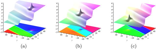
Figure 5. Hybrid solution between 1-lump and 2-solitons with ${\rho }_{2}={\rho }_{1}^{* }=\tfrac{1}{5}-i$, ${h}_{3}=1,{\rho }_{3}=-\tfrac{1}{2},{h}_{4}=1$, ${\rho }_{4}=-\tfrac{1}{2}$, ${\chi }_{3}^{0}=-20$, ${\chi }_{4}^{0}=20$, δ1 = 1, δ2 = −1, at (a) t = −10; (b) t = 0; (c) t = 10. |
4.3. A hybrid solution between 2-lumps and 1-soliton
The hybrid solution consists of 2-lumps and 1-soliton can be generated from 5-soliton solution. To begin with, let N = 5 in the equation (6 ) and we obtain the 5-soliton solution f5. Then inserting the conditions ${\chi }_{1}^{0}$ = ${\chi }_{2}^{0}$ = ${\chi }_{3}^{0}$ = ${\chi }_{4}^{0}={\rm{i}}\pi $, h1, h2, h3, h4 → 0, ${\rho }_{3}={\rho }_{1}^{* }$ = a1 − b1i and ${\rho }_{4}={\rho }_{2}^{* }$ = a2 − b2i into f5. The function f5 can be rewritten as24 )–(26 ) into the variable transformation $u=2{\left(\mathrm{ln}f\right)}_{x}$, we gain the hybrid solution consists of 2-lumps and 1-soliton as shown in figure 6. In figure 6, the 2-lump waves move gradually from the right side of the soliton wave to its left side. The shape and amplitude of the lump waves do not change before and after they completely cross the soliton wave.
$\begin{eqnarray}\begin{array}{l}{f}_{\mathrm{2,1}}={\beta }_{1}{\beta }_{2}{\beta }_{3}{\beta }_{4}+{Q}_{12}{\beta }_{3}{\beta }_{4}+{Q}_{13}{\beta }_{2}{\beta }_{4}+{Q}_{14}{\beta }_{2}{\beta }_{3}\\ \quad +{Q}_{23}{\beta }_{1}{\beta }_{4}+{Q}_{24}{\beta }_{1}{\beta }_{3}+{Q}_{34}{\beta }_{1}{\beta }_{2}+{Q}_{12}{Q}_{34}\\ \quad +{Q}_{13}{Q}_{24}+{Q}_{14}{Q}_{23}+{{\rm{e}}}^{{\chi }_{5}}\cdot \left({Q}_{15}{Q}_{25}{Q}_{35}{Q}_{45}\right.\\ \quad +{Q}_{15}{Q}_{25}{Q}_{35}{\beta }_{4}+{Q}_{15}{Q}_{25}{Q}_{45}{\beta }_{3}+{Q}_{15}{Q}_{35}{Q}_{45}{\beta }_{2}\\ \quad +{Q}_{25}{Q}_{35}{Q}_{45}{\beta }_{1}+{Q}_{15}{Q}_{25}{\beta }_{3}{\beta }_{4}+{Q}_{15}{Q}_{35}{\beta }_{2}{\beta }_{4}\\ \quad +{Q}_{15}{Q}_{45}{\beta }_{2}{\beta }_{3}+{Q}_{25}{Q}_{35}{\beta }_{1}{\beta }_{4}\\ \quad +{Q}_{25}{Q}_{45}{\beta }_{1}{\beta }_{3}+{Q}_{35}{Q}_{45}{\beta }_{1}{\beta }_{2}\\ \quad +{Q}_{15}{\beta }_{2}{\beta }_{3}{\beta }_{4}+{Q}_{25}{\beta }_{1}{\beta }_{3}{\beta }_{4}\\ \quad +{Q}_{35}{\beta }_{1}{\beta }_{2}{\beta }_{4}+{Q}_{45}{\beta }_{1}{\beta }_{2}{\beta }_{3}\\ \quad +{\beta }_{1}{\beta }_{2}{\beta }_{3}{\beta }_{4}+{Q}_{12}{Q}_{35}{Q}_{45}+{Q}_{12}{Q}_{35}{\beta }_{4}+{Q}_{12}{Q}_{45}{\beta }_{3}\\ \quad +{Q}_{12}{\beta }_{3}{\beta }_{4}+{Q}_{13}{Q}_{25}{Q}_{45}+{Q}_{13}{Q}_{25}{\beta }_{4}+{Q}_{13}{Q}_{45}{\beta }_{2}\\ \quad +{Q}_{13}{\beta }_{2}{\beta }_{4}+{Q}_{14}{Q}_{25}{Q}_{35}+{Q}_{14}{Q}_{25}{\beta }_{3}+{Q}_{14}{Q}_{35}{\beta }_{2}\\ \quad +{Q}_{14}{\beta }_{2}{\beta }_{3}+{Q}_{15}{Q}_{23}{Q}_{45}+{Q}_{15}{Q}_{23}{\beta }_{4}+{Q}_{15}{Q}_{24}{Q}_{35}\\ \quad +{Q}_{15}{Q}_{24}{\beta }_{3}+{Q}_{15}{Q}_{25}{Q}_{34}+{Q}_{15}{Q}_{34}{\beta }_{2}\\ \quad +{Q}_{23}{Q}_{45}{\beta }_{1}+{Q}_{23}{\beta }_{1}{\beta }_{4}+{Q}_{24}{Q}_{35}{\beta }_{1}\\ \quad +{Q}_{24}{\beta }_{1}{\beta }_{3}+{Q}_{25}{Q}_{34}{\beta }_{1}+{Q}_{34}{\beta }_{1}{\beta }_{2}+{Q}_{12}{Q}_{34}\\ \quad \left.+{Q}_{13}{Q}_{24}+{Q}_{14}{Q}_{23}\right),\end{array}\end{eqnarray}$
with $\begin{eqnarray}\begin{array}{l}{\beta }_{1}=x+{\rho }_{1}y+\left(-{\delta }_{1}{\rho }_{1}-\displaystyle \frac{{\delta }_{2}}{{\rho }_{1}}\right)t,\\ {\beta }_{2}=x+{\rho }_{2}y+\left(-{\delta }_{1}{\rho }_{2}-\displaystyle \frac{{\delta }_{2}}{{\rho }_{2}}\right)t,\\ {\beta }_{3}=x+{\rho }_{3}y+\left(-{\delta }_{1}{\rho }_{3}-\displaystyle \frac{{\delta }_{2}}{{\rho }_{3}}\right)t,\\ {\beta }_{4}=x+{\rho }_{4}y+\left(-{\delta }_{1}{\rho }_{4}-\displaystyle \frac{{\delta }_{2}}{{\rho }_{4}}\right)t,\\ {\chi }_{5}={h}_{5}\left(x+{\rho }_{5}y+(-{h}_{5}^{2}-{\delta }_{1}{\rho }_{5}-\displaystyle \frac{{\delta }_{2}}{{\rho }_{5}})t\right)+{\chi }_{5}^{0},\\ {Q}_{12}=\displaystyle \frac{6{\rho }_{1}{\rho }_{2}({\rho }_{1}+{\rho }_{2})}{{\delta }_{2}{\left({\rho }_{1}-{\rho }_{2}\right)}^{2}},\\ {Q}_{13}=\displaystyle \frac{6{\rho }_{1}{\rho }_{3}({\rho }_{1}+{\rho }_{3})}{{\delta }_{2}{\left({\rho }_{1}-{\rho }_{3}\right)}^{2}},{Q}_{14}=\displaystyle \frac{6{\rho }_{1}{\rho }_{4}({\rho }_{1}+{\rho }_{4})}{{\delta }_{2}{\left({\rho }_{1}-{\rho }_{4}\right)}^{2}},\\ {Q}_{23}=\displaystyle \frac{6{\rho }_{2}{\rho }_{3}({\rho }_{2}+{\rho }_{3})}{{\delta }_{2}{\left({\rho }_{2}-{\rho }_{3}\right)}^{2}},\\ {Q}_{24}=\displaystyle \frac{6{\rho }_{2}{\rho }_{4}({\rho }_{2}+{\rho }_{4})}{{\delta }_{2}{\left({\rho }_{2}-{\rho }_{4}\right)}^{2}},{Q}_{34}=\displaystyle \frac{6{\rho }_{3}{\rho }_{4}({\rho }_{3}+{\rho }_{4})}{{\delta }_{2}{\left({\rho }_{3}-{\rho }_{4}\right)}^{2}},\\ {Q}_{15}=\displaystyle \frac{-6{\rho }_{1}{\rho }_{5}({\rho }_{1}+{\rho }_{5})}{3{\rho }_{1}{\rho }_{5}^{2}{h}_{5}^{2}-{\delta }_{2}{\left({\rho }_{1}-{\rho }_{5}\right)}^{2}},\\ {Q}_{25}=\displaystyle \frac{-6{\rho }_{2}{\rho }_{5}({\rho }_{2}+{\rho }_{5})}{3{\rho }_{2}{\rho }_{5}^{2}{h}_{5}^{2}-{\delta }_{2}{\left({\rho }_{2}-{\rho }_{5}\right)}^{2}},\\ {Q}_{35}=\displaystyle \frac{-6{\rho }_{3}{\rho }_{5}({\rho }_{3}+{\rho }_{5})}{3{\rho }_{3}{\rho }_{5}^{2}{h}_{5}^{2}-{\delta }_{2}{\left({\rho }_{3}-{\rho }_{5}\right)}^{2}},\\ {Q}_{45}=\displaystyle \frac{-6{\rho }_{4}{\rho }_{5}({\rho }_{4}+{\rho }_{5})}{3{\rho }_{4}{\rho }_{5}^{2}{h}_{5}^{2}-{\delta }_{2}{\left({\rho }_{4}-{\rho }_{5}\right)}^{2}}.\end{array}\end{eqnarray}$
Taking $\begin{eqnarray}\begin{array}{l}{a}_{1}=\displaystyle \frac{1}{3},{b}_{1}=\displaystyle \frac{4}{3},{a}_{2}=\displaystyle \frac{1}{20},{b}_{2}=\displaystyle \frac{4}{3},{h}_{5}=\displaystyle \frac{3}{4},\\ {\rho }_{5}=-\displaystyle \frac{5}{4},{\chi }_{5}^{0}=0,{\delta }_{1}=1,{\delta }_{2}=-1.\end{array}\end{eqnarray}$
Substituting equations (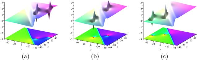
Figure 6. Hybrid solution between 2-lumps and 1-soliton with ${\rho }_{3}={\rho }_{1}^{* }=\tfrac{1}{3}-\tfrac{4}{3}{\rm{i}},{\rho }_{4}={\rho }_{2}^{* }=\tfrac{1}{20}-\tfrac{4}{3}{\rm{i}},{h}_{5}=\tfrac{3}{4},{\rho }_{5}=-\tfrac{5}{4},{\chi }_{5}^{0}=0$, δ1 = 1, δ2 = −1, at (a) t = −20; (b) t = 0; (c) t = 20. |
5. T-order breather solutions
The parameters of the N-soliton solution expression in this section need to be taken as conjugate if we want to obtain the T-order breather solutions (N = 2T). We set the following parameters:6 ), the N-soliton solutions will be transformed into T-order breather solutions.
$\begin{eqnarray}\begin{array}{l}N=2T,{h}_{i+T}={h}_{i}^{* },{\rho }_{i+T}={\rho }_{i}^{* },{\chi }_{i+T}^{0}={\left({\chi }_{i}^{0}\right)}^{* }\\ .(i=1,2,\ldots ,T).\end{array}\end{eqnarray}$
Bringing these constraints into the equation (5.1. 1st-order breather solution
Let N = 2T = 2 in the equation (6 ), the 2-soliton solution has the following form
$\begin{eqnarray}{f}_{2-{soliton}}=1+{{\rm{e}}}^{{\chi }_{1}}+{{\rm{e}}}^{{\chi }_{2}}+{{\rm{e}}}^{{\chi }_{1}+{\chi }_{2}+{{\rm{\Omega }}}_{12}}.\end{eqnarray}$
Taking the parameters in a conjugate form: $\begin{eqnarray}\begin{array}{l}{h}_{2}={h}_{1}^{* }=a-b{\rm{i}},{\rho }_{2}={\rho }_{1}^{* }=c-d{\rm{i}},\\ {\chi }_{2}^{0}={\left({\chi }_{1}^{0}\right)}^{* }=0.\end{array}\end{eqnarray}$
After the calculation, f2−soliton will be transformed into the following form of the 1-order breather solution $\begin{eqnarray}{f}_{1-{breather}}=1+{{\rm{e}}}^{{{\rm{\Omega }}}_{12}}{{\rm{e}}}^{2{\zeta }_{1}}+2{{\rm{e}}}^{{\zeta }_{1}}\cos {\zeta }_{2},\end{eqnarray}$
with $\begin{eqnarray}\begin{array}{l}{{\rm{e}}}^{{{\rm{\Omega }}}_{12}}=\displaystyle \frac{3{\rho }_{1}{\rho }_{2}({h}_{1}-{h}_{2})({h}_{1}{\rho }_{1}-{h}_{2}{\rho }_{2})-{\delta }_{2}{\left({\rho }_{1}-{\rho }_{2}\right)}^{2}}{3{\rho }_{1}{\rho }_{2}({h}_{1}+{h}_{2})({h}_{1}{\rho }_{1}+{h}_{2}{\rho }_{2})-{\delta }_{2}{\left({\rho }_{1}-{\rho }_{2}\right)}^{2}}\\ \quad =\displaystyle \frac{-3b({c}^{2}+{d}^{2})({ad}+{bc})+{\delta }_{2}{d}^{2}}{3a({c}^{2}+{d}^{2})({ac}-{bd})+{\delta }_{2}{d}^{2}},\\ {\zeta }_{1}={ax}+({ac}-{bd})y+\left(-a({a}^{2}-3{b}^{2})\right.\\ \quad \left.-({ac}-{bd}){\delta }_{1}-\displaystyle \frac{{ac}+{bd}}{{c}^{2}+{d}^{2}}{\delta }_{2}\right)t,\\ {\zeta }_{2}={bx}+({ad}+{bc})y+\left(-b(3{a}^{2}-{b}^{2})\right.\\ \quad \left.-({ad}+{bc}){\delta }_{1}-\displaystyle \frac{{ad}-{bc}}{{c}^{2}+{d}^{2}}{\delta }_{2}\right)t.\end{array}\end{eqnarray}$
Due to the different types of parameters of {h1, h2, ρ1, ρ2} we choose, different spatial arrangements of 1st-order breather solutions exist. We discuss the parameters in the following types:| 1. | (1) When both hi and ρi are pure imaginary numbers, which means a = 0 and c = 0, the 1st-order breather solution presents periodic on the x-axis and fixed on the y-axis, as shown in figure 7(a). |
| 2. | (2) When hi is a pure real number and ρi is a pure imaginary number, which means b = 0 and c = 0, the 1st-order breather solution presents periodic on the y-axis and fixed on the x-axis, as shown in figure 7(b). |
| 3. | (3) When both hi and ρi are complex numbers, which means a, b, c, d ≠ 0, the 1st-order breather solution parallel to the line ax + (ac − bd)y = 0, see figure 7(c). |
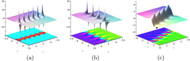
Figure 7. Three types of first-order breather solutions at t = 0 with ${\chi }_{2}^{0}={\left({\chi }_{1}^{0}\right)}^{* }=0$, δ1 = 1, δ2 = −1, (a) ${h}_{2}={h}_{1}^{* }=-3{\rm{i}},{\rho }_{2}={\rho }_{1}^{* }=-{\rm{i}};$ (b) ${h}_{2}={h}_{1}^{* }=1,{\rho }_{2}={\rho }_{1}^{* }=-2{\rm{i}};$ (c) ${h}_{2}={h}_{1}^{* }=\tfrac{1}{3}-{\rm{i}},{\rho }_{2}={\rho }_{1}^{* }=\tfrac{2}{5}-{\rm{i}}$. |
5.2. 2nd-order breather solution
When N = 2T = 4 in N-soliton solutions (6 ) with conditions (27 ), 2nd-order breather solution is determined as
$\begin{eqnarray}\begin{array}{l}{f}_{2-{breather}}=1+{{\rm{e}}}^{{\chi }_{1}}+{{\rm{e}}}^{{\chi }_{2}}+{{\rm{e}}}^{{\chi }_{3}}+{{\rm{e}}}^{{\chi }_{4}}+{{\rm{e}}}^{{\chi }_{1}+{\chi }_{2}+{{\rm{\Omega }}}_{12}}\\ \quad +{{\rm{e}}}^{{\chi }_{1}+{\chi }_{3}+{{\rm{\Omega }}}_{13}}+{{\rm{e}}}^{{\chi }_{1}+{\chi }_{4}+{{\rm{\Omega }}}_{14}}\\ \quad +{{\rm{e}}}^{{\chi }_{2}+{\chi }_{3}+{{\rm{\Omega }}}_{23}}\\ \quad +{{\rm{e}}}^{{\chi }_{2}+{\chi }_{4}+{{\rm{\Omega }}}_{23}}+{{\rm{e}}}^{{\chi }_{3}+{\chi }_{4}+{{\rm{\Omega }}}_{34}}+{{\rm{e}}}^{{\chi }_{1}+{\chi }_{2}+{\chi }_{3}+{{\rm{\Omega }}}_{12}+{{\rm{\Omega }}}_{13}+{{\rm{\Omega }}}_{23}}\\ \quad +{{\rm{e}}}^{{\chi }_{1}+{\chi }_{2}+{\chi }_{4}+{{\rm{\Omega }}}_{12}+{{\rm{\Omega }}}_{14}+{{\rm{\Omega }}}_{24}}\\ \quad +{{\rm{e}}}^{{\chi }_{1}+{\chi }_{3}+{\chi }_{4}+{{\rm{\Omega }}}_{13}+{{\rm{\Omega }}}_{14}+{{\rm{\Omega }}}_{34}}+{{\rm{e}}}^{{\chi }_{2}+{\chi }_{3}+{\chi }_{4}+{{\rm{\Omega }}}_{23}+{{\rm{\Omega }}}_{24}+{{\rm{\Omega }}}_{34}}\\ \quad +{{\rm{e}}}^{{\chi }_{1}+{\chi }_{2}+{\chi }_{3}+{\chi }_{4}+{{\rm{\Omega }}}_{12}+{{\rm{\Omega }}}_{13}+{{\rm{\Omega }}}_{14}+{{\rm{\Omega }}}_{23}+{{\rm{\Omega }}}_{24}+{{\rm{\Omega }}}_{34}}.\end{array}\end{eqnarray}$
We assume that parameters have a conjugate relation and set δ1 = 1, δ2 = −1, ${h}_{3}={h}_{1}^{* }$ = $\tfrac{1}{3}+\tfrac{1}{2}{\rm{i}}$, ${\rho }_{3}={\rho }_{1}^{* }=-\tfrac{2}{3}{\rm{i}}$, ${h}_{4}={h}_{2}^{* }=\tfrac{1}{3}-\tfrac{1}{2}{\rm{i}}$, ${\rho }_{4}={\rho }_{2}^{* }=-\tfrac{2}{3}{\rm{i}}$, ${\chi }_{1}^{0}={\chi }_{2}^{0}$ = ${\chi }_{3}^{0}\,={\chi }_{4}^{0}=0$ in f2−breather. The 2nd-order breather solution consisting of two breather waves is derived in figure 8. As previously stated, the 1st-order breather wave has three distinct structures. Therefore, it leads to the occurrence of multiple spatial arrangements between two breather waves. Such as parallel to the x-axis, parallel to the y-axis, and intersecting, where mutual perpendicularity (see figure 8) is a special kind of intersection. Here, we make graphs and observations only for the case of two waves perpendicular to each other.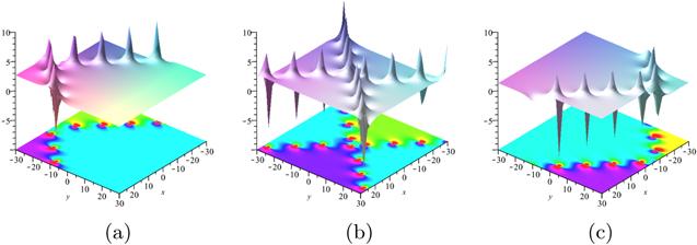
Figure 8. 2nd-order breather solution with δ1 = 1, δ2 = −1, ${h}_{3}={h}_{1}^{* }=\tfrac{1}{3}+\tfrac{1}{2}{\rm{i}}$, ${\rho }_{3}={\rho }_{1}^{* }=-\tfrac{2}{3}{\rm{i}}$, ${h}_{4}={h}_{2}^{* }=\tfrac{1}{3}-\tfrac{1}{2}{\rm{i}}$, ${\rho }_{4}={\rho }_{2}^{* }=-\tfrac{2}{3}{\rm{i}}$, ${\chi }_{1}^{0}={\chi }_{2}^{0}={\chi }_{3}^{0}={\chi }_{4}^{0}=0$ at (a) t = −10; (b) t = 0; (c) t = 10. |
5.3. 3rd-order breather solution
The case of N = 2T = 6 is similar to the above discussion. We take δ1 = 1, δ2 = −1, ${h}_{4}={h}_{1}^{* }=1-\tfrac{4}{3}{\rm{i}}$, ${\rho }_{4}={\rho }_{1}^{* }=-\tfrac{3}{2}{\rm{i}}$, ${h}_{5}={h}_{2}^{* }=1+\tfrac{5}{3}{\rm{i}}$, ${\rho }_{5}={\rho }_{2}^{* }=-\tfrac{6}{5}{\rm{i}}$, ${h}_{6}={h}_{3}^{* }=1$, ${\rho }_{6}\,={\rho }_{3}^{* }\,=-\tfrac{3}{2}{\rm{i}}$, ${\chi }_{1}^{0}={\chi }_{2}^{0}$ = ${\chi }_{3}^{0}={\chi }_{4}^{0}$ = ${\chi }_{5}^{0}={\chi }_{6}^{0}=0$ in formula (6 ). The images of the 3rd-order breather solution are shown in figure 9.
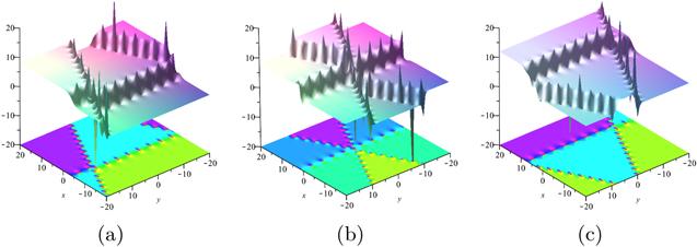
Figure 9. 3rd-order breather solution with δ1 = 1, δ2 = −1, ${h}_{4}={h}_{1}^{* }=1-\tfrac{4}{3}{\rm{i}}$, ${\rho }_{4}={\rho }_{1}^{* }=-\tfrac{3}{2}{\rm{i}}$, ${h}_{5}={h}_{2}^{* }=1+\tfrac{5}{3}{\rm{i}}$, ${\rho }_{5}={\rho }_{2}^{* }=-\tfrac{6}{5}{\rm{i}}$, ${h}_{6}={h}_{3}^{* }=1$, ${\rho }_{6}={\rho }_{3}^{* }$ = $-\tfrac{3}{2}{\rm{i}}$, ${\chi }_{1}^{0}$ = ${\chi }_{2}^{0}={\chi }_{3}^{0}$ = ${\chi }_{4}^{0}={\chi }_{5}^{0}$ = ${\chi }_{6}^{0}=0$ at (a) t = −5; (b) t = 0; (c) t = 5. |
6. Hybrid solutions between breathers and solitons
Deriving the interaction solutions of the T-order breathers and K-solitons by letting
$\begin{eqnarray}\begin{array}{l}N=2T+K,{h}_{j+T}={h}_{j}^{* },{\rho }_{j+T}={\rho }_{j}^{* },\\ {\chi }_{j+T}^{0}={\left({\chi }_{j}^{0}\right)}^{* },(j=1,2,\ldots ,T)\end{array}\end{eqnarray}$
is the purpose of the study in this section, where T and K are the positive integers, hs, ρs and ${\chi }_{s}^{0}$ are the real constants (s = 2T + 1, …2T + K).6.1. A hybrid solution between 1-breather and 1-soliton
To get more detailed results of the interaction solution between 1-breather and 1-soliton, we need to take the parameters as34 ) into it, we obtain the interaction solution as shown in figure 10. When a1c1 − b1d1 = a1c3, the 1st-order breather is parallel to the 1-soliton on the (x, y) plane, as shown in figure 10(a). When ${a}_{1}{c}_{1}-{b}_{1}{d}_{1}=-\tfrac{{a}_{1}}{{c}_{3}}$, the 1st-order breather and the 1-soliton are perpendicular to each other on the (x, y) plane, as shown in figure 10(b). When neither of the above is satisfied, they are intersected on the (x, y) plane, as shown in figure 10(c).
$\begin{eqnarray}\begin{array}{l}N=3,T=1,K=1,\\ {h}_{2}={h}_{1}^{* }={a}_{1}-{b}_{1}{\rm{i}},{h}_{3}={a}_{3},\\ {\rho }_{2}={\rho }_{1}^{* }={c}_{1}-{d}_{1}{\rm{i}},{\rho }_{3}={c}_{3},{\chi }_{1}^{0}={\chi }_{2}^{0}={\chi }_{3}^{0}=0.\end{array}\end{eqnarray}$
Bringing f3−soliton into $u=2{\left(\mathrm{ln}f\right)}_{x}$ after inserting parameters (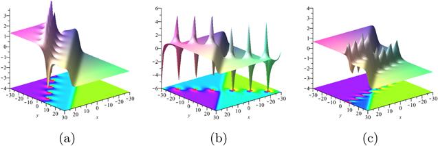
Figure 10. Hybrid solution between 1-breather and 1-soliton with δ1 = 1, δ2 = −1, (a)${h}_{2}={h}_{1}^{* }=\tfrac{1}{3}-\tfrac{1}{2}{\rm{i}}$, ${h}_{3}=-1,{\rho }_{2}={\rho }_{1}^{* }=-\tfrac{2}{3}{\rm{i}}$, ${\rho }_{3}=-1,{\chi }_{1}^{0}={\chi }_{2}^{0}={\chi }_{3}^{0}=0,t=-5;$ (b)${h}_{2}={h}_{1}^{* }=\tfrac{1}{3}+\tfrac{1}{2}{\rm{i}}$, ${h}_{3}=-1,{\rho }_{2}={\rho }_{1}^{* }=-\tfrac{2}{3}{\rm{i}}$, ρ3 = −1, ${\chi }_{1}^{0}={\chi }_{2}^{0}={\chi }_{3}^{0}=0,t=0;$ (c)${h}_{2}={h}_{1}^{* }=\tfrac{1}{6}-\tfrac{2}{3}{\rm{i}}$, ${h}_{3}=-1,{\rho }_{2}={\rho }_{1}^{* }=\tfrac{2}{5}-{\rm{i}}$, ${\rho }_{3}=-1,{\chi }_{1}^{0}={\chi }_{2}^{0}={\chi }_{3}^{0}=0,t=0$. |
6.2. A hybrid solution between 1-breather and 2-solitons
Now, we set35 ) into the expression f4−soliton given by equation (6 ), an interaction solution between 1-breather and 2-solitons is obtained, which is shown in figure 11. Figure 11 shows the evolution of the hybrid solution at time t = −3, 0, 3. From these figures, we can see that the breather wave and two soliton waves move in opposite directions.
$\begin{eqnarray}\begin{array}{l}N=4,T=1,K=2,{h}_{2}={h}_{1}^{* }={a}_{1}-{b}_{1}{\rm{i}},\\ {h}_{3}={a}_{3},{h}_{4}={a}_{4},\\ {\rho }_{2}={\rho }_{1}^{* }={c}_{1}-{d}_{1}{\rm{i}},{\rho }_{3}={c}_{3},{\rho }_{4}={c}_{4},\\ {\chi }_{1}^{0}={\chi }_{2}^{0}={\chi }_{3}^{0}={\chi }_{4}^{0}=0.\end{array}\end{eqnarray}$
Bringing parameters (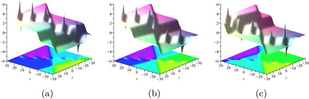
Figure 11. Hybrid solution between 1-breather and 2-solitons with δ1 = 1, δ2 = −1, ${h}_{2}={h}_{1}^{* }=\tfrac{1}{4}-\tfrac{1}{3}{\rm{i}}$, h3 = 1, h4 = −1, ${\rho }_{2}={\rho }_{1}^{* }=\tfrac{1}{10}-\tfrac{4}{3}{\rm{i}}$, ${\rho }_{3}=-\tfrac{1}{5}$, ${\rho }_{4}=1,{\chi }_{1}^{0}={\chi }_{2}^{0}={\chi }_{3}^{0}=0$, at (a) t = −3; (b) t = 0; (c) t = 3. |
6.3. A hybrid solution between 2-breathers and 1-soliton
Next, we choose
$\begin{eqnarray}\begin{array}{l}N=5,T=2,K=1,{h}_{3}={h}_{1}^{* }={a}_{1}-{b}_{1}{\rm{i}},\\ {h}_{4}={h}_{2}^{* }={a}_{2}-{b}_{2}{\rm{i}},\\ {h}_{5}={a}_{5},{\rho }_{5}={c}_{5},\\ {\rho }_{3}={\rho }_{1}^{* }={c}_{1}-{d}_{1}{\rm{i}},{\rho }_{4}={\rho }_{2}^{* }={c}_{2}-{d}_{2}{\rm{i}},\\ {\chi }_{1}^{0}={\chi }_{2}^{0}={\chi }_{3}^{0}={\chi }_{4}^{0}={\chi }_{5}^{0}=0.\end{array}\end{eqnarray}$
Taking them into 5-soliton solution, then we can turn the soliton solution into the hybrid solution between 2-breathers and 1-soliton. Figure 12 shows the evolution of the hybrid solution at time t = −3, 0, 3.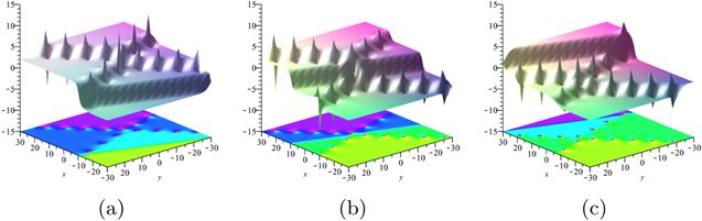
Figure 12. Hybrid solution between 2-breathers and 1-soliton with δ1 = 1, δ2 = −1, ${h}_{3}={h}_{1}^{* }=\tfrac{1}{2}-\tfrac{1}{2}{\rm{i}}$, ${h}_{4}={h}_{2}^{* }=\tfrac{1}{2}+\tfrac{1}{6}{\rm{i}}$, h5 = −2, ${\rho }_{3}={\rho }_{1}^{* }={\rho }_{4}={\rho }_{2}^{* }=-{\rm{i}}$, ${\rho }_{5}=-\tfrac{1}{3}$, ${\chi }_{1}^{0}={\chi }_{2}^{0}={\chi }_{3}^{0}={\chi }_{4}^{0}={\chi }_{5}^{0}=0$, at (a) t = −3; (b) t = 0; (c) t = 3. |
7. Hybrid solutions between lumps and breathers
In this section, we find the hybrid solutions composed of the T-order breathers and M-order lumps with the conditions
$\begin{eqnarray}\begin{array}{l}N=2T+2M,{h}_{j+T}={h}_{j}^{* }={a}_{j}-{b}_{j}{\rm{i}},\\ {\rho }_{j+T}={\rho }_{j}^{* }={c}_{j}-{d}_{j}{\rm{i}},{\chi }_{j+T}^{0}={\left({\chi }_{j}^{0}\right)}^{* },\\ {h}_{2T+1},\ldots ,{h}_{2T+2M}\to 0,{\rho }_{M+l}={\rho }_{l}^{* }={c}_{l}-{d}_{l}{\rm{i}},\\ {\chi }_{2T+1}^{0}=...={\chi }_{2T+2M}^{0}={\rm{i}}\pi ,\\ (j=1,2,\ldots ,T,l=2T+1,2T+2,\ldots ,2T+M).\end{array}\end{eqnarray}$
where T and M are the positive integers, aj, bj, c, d and ${\chi }_{j}^{0}$ are the real constants.7.1. A hybrid solution between 1-breather and 1-lump
If the parameters of the equation (6 ) satisfy
$\begin{eqnarray}\begin{array}{l}N=4,T=1,M=1,{h}_{2}={h}_{1}^{* }={a}_{1}-{b}_{1}{\rm{i}},\\ {\rho }_{2}={\rho }_{1}^{* }={c}_{1}-{d}_{1}{\rm{i}},\\ {h}_{3},{h}_{4}\to 0,{\rho }_{4}={\rho }_{3}^{* }={c}_{3}-{d}_{3}{\rm{i}},{\chi }_{2}^{0}={\chi }_{1}^{0}=0,\\ {\chi }_{3}^{0}={\chi }_{4}^{0}={\rm{i}}\pi ,\end{array}\end{eqnarray}$
the interaction solution will be obtained, which consists of a breather and a lump solution (see figure 13). Figure 13 demonstrates that the breather wave and lump wave move in opposite directions along the x-axis. It can also be seen that the velocity and shape of the two waves after the collision are the same as before.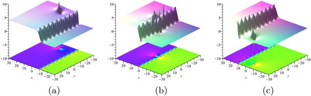
Figure 13. Hybrid solution between 1-breather and 1-lump with δ1 = 1, δ2 = −1, ${h}_{2}={h}_{1}^{* }=1$, ${\rho }_{2}={\rho }_{1}^{* }={\rm{i}}$, ${\rho }_{4}={\rho }_{3}^{* }=\tfrac{1}{10}-{\rm{i}}$, ${\chi }_{2}^{0}={\chi }_{1}^{0}=0$, at (a) t = −10; (b) t = 0; (c) t = 10. |
8. Conclusions
The (2+1)-dimensional eBLMP equation is the main subject of this work. Via the bilinear transformation formula, we can easily find the bilinear form and the expressions of the N-soliton solutions of the equation. Using the long-wave limit method, we can effectively find the higher-order lump solutions and analyze the situations of 1-lump, 2-lump, and 3-lump solutions. The expressions and images of solutions can describe the dynamic characteristics. We discover that the wave follows a specific trajectory with uniform velocity. When multiple waves move simultaneously, a collision happens accompanied by morphological changes. After the collision, the waves separate from each other and return to their original shapes (see figures 1–3). Taking the parameters as conjugate relations, we can construct high-order breather solutions. The 1st-order breather solutions contain three different types of spatial arrangements due to the diverse parameter settings: parallel to the x-axis, parallel to the y-axis, and the general case. This result leads to multiple spatial combinations of high-order breather solutions. The evolution and collision of solutions can be seen in graphs (see figures 7–9). Furthermore, we analyze the interactions between other solutions, such as lump-soliton solutions (see figures 4–6), breather-soliton solutions (see figures 10–12), and lump-breather solutions (see figure 13). With the help of these solutions, we can more effectively explore nonlinear phenomena. The figures show the changes caused by different kinds of solutions colliding. The methods we adopted in this article are remarkable for solving nonlinear systems and the solutions we obtained can explain physical phenomena in nature.