New physical structures and patterns to the optical solutions of the nonlinear Schr&#xF6;dinger equation with a higher dimension

Karmina K Ali; Abdullahi Yusuf; Marwan Alquran; Sibel Tarla

doi:10.1088/1572-9494/acde69

2023 , Vol. 75 >Issue 8: 85003

DOI: https://doi.org/10.1088/1572-9494/acde69

Mathematical Physics

New physical structures and patterns to the optical solutions of the nonlinear Schrödinger equation with a higher dimension

Karmina K Ali ¹^,² ,
Abdullahi Yusuf ³^,⁴^,⁵ ,
Marwan Alquran ^,⁶^,^∗ ,
Sibel Tarla ⁷

Expand

¹Department of Mathematics, Faculty of Science, University of Zakho, Zakho, Iraq
²Department of Computer Science, College of Science, Knowledge University, Erbil 44001, Iraq
³Department of Computer Engineering, Biruni University, Istanbul, Turkey
⁴Department of Computer Science and Mathematics, Lebanese American University, Beirut, Lebanon
⁵Department of Mathematics, Near East University TRNC, Mersin 10, Nicosia 99138, Turkey
⁶Department of Mathematics and Statistics, Jordan University of Science & Technology, Irbid 22110, Jordan
⁷Department of Mathematics, Faculty of Science, Firat University, Elazig, Turkey

^∗Author to whom any correspondence should be addressed.

Received date: 2023-01-14

Revised date: 2023-04-20

Accepted date: 2023-06-15

Online published: 2023-07-20

Copyright

Fold

Abstract

It is commonly recognized that, despite current analytical approaches, many physical aspects of nonlinear models remain unknown. It is critical to build more efficient integration methods to design and construct numerous other unknown solutions and physical attributes for the nonlinear models, as well as for the benefit of the largest audience feasible. To achieve this goal, we propose a new extended unified auxiliary equation technique, a brand-new analytical method for solving nonlinear partial differential equations. The proposed method is applied to the nonlinear Schrödinger equation with a higher dimension in the anomalous dispersion. Many interesting solutions have been obtained. Moreover, to shed more light on the features of the obtained solutions, the figures for some obtained solutions are graphed. The propagation characteristics of the generated solutions are shown. The results show that the proper physical quantities and nonlinear wave qualities are connected to the parameter values. It is worth noting that the new method is very effective and efficient, and it may be applied in the realisation of novel solutions.

Key words： exact solutions; nonlinear Schrödinger equation; new extended unified auxiliary equation method; Jacobi elliptic functions

Cite this article

Karmina K Ali , Abdullahi Yusuf , Marwan Alquran , Sibel Tarla . New physical structures and patterns to the optical solutions of the nonlinear Schrödinger equation with a higher dimension[J]. Communications in Theoretical Physics, 2023 , 75(8) : 085003 . DOI: 10.1088/1572-9494/acde69

1. Introduction

Nonlinear equations are organically investigated in many fields of research, more especially in applied and computational sciences. The application of nonlinear equations in the sense of both ordinary and partial differential equations (PDEs) in mathematical modeling has sparked interest in differential equations. The PDEs are an essential instrument for extensively investigating the features of physical processes [1–4]. The Schrödinger-type governing equation, which is critical in the disciplines of optics, fiber optics, mathematical physics, telecommunication engineering, and plasma technology, is one of the excellent ways to more accurately understand the complicated physical nonlinear model [5–7]. Due to the crucial role that exact solutions play in accurately representing the physical properties of nonlinear systems in applied mathematics, the derivation of analytical solutions for the Schrödinger and other water wave equations is a crucial study area [8–20].

In the 19th century, many approaches for constructing explicit solutions to differential equations were devised. There are various applications in the theoretical study of PDEs. It should be emphasized that extremely complex equations are beyond the capabilities of even supercomputers. In these situations, we try to gather qualitative information from the solution. The formulation of the equation and its indicated side conditions is also an important consideration. Typically, the equations are developed from a physical or technical problem. It is not immediately obvious that the model is consistent in the sense that it leads to solvable PDEs [21–31].

The nonlinear Schrodinger equation (NLSE) is one form of PDEs, and studies on NLSEs have achieved some remarkable success for decades due to its vast variety of applications. Nonlinear optics, Bose–Einstein delicacy, and fluid dynamics are all represented by distinct forms of NLSEs, as well as numerous more in different areas. The distinguishing element of the varieties of NLSEs discovered is some form of nonlinearity to create more light on the disruption that happens when the electromagnetic pulses spread at the optical extreme. They contribute to understanding the underlying physics phenomena of ultrashort pulses in nonlinear and dispersion media. The perturbation method, which is used under certain conditions to generate analytical solutions; the inverse scattering method for classical solitons; the perturbation principle for multidimensional NLSEs in the field of molecular physics; the dam-break approximation for unrelated solitons; and the dam-break approximation for unrelated solitons are among the robust methods used for similar NLSEs [32–35].

Various concepts have demonstrated that optical solitons may be employed as an information carrier for long-distance optical fiber communication and optical data transfer. Two of the most important physical factors in single-mode fiber are group velocity dispersion and self-phase modulation. It eliminates pulse broadening due to group velocity dispersion, and self-phase modulation promotes pulse compression [32–35]. Based on the facts given, it can be concluded that, despite current tools and analytical schemes in the literature, many physical properties remain undiscovered and must be researched and developed for the benefit of the broadest possible audience.

To that purpose, we present a new extended unified auxiliary equation approach, a novel analytical scheme, a brand-new analytical method for solving nonlinear PDEs. The new approach is incredibly effective and efficient, and it may be used to generate many interesting solutions.

The new method is applied to the NLSEs with higher dimension in the anomalous dispersion regime, which is defined by [36]

(1.1)$\begin{eqnarray}\begin{array}{l}{\rm{i}}\displaystyle \frac{\partial \psi }{\partial t}+{\lambda }_{1}\displaystyle \frac{{\partial }^{2}\psi }{\partial {x}^{2}}+{\lambda }_{2}\displaystyle \frac{{\partial }^{2}\psi }{\partial {y}^{2}}+{\lambda }_{3}| \psi {| }^{2}\psi \\ \qquad +{\lambda }_{4}\displaystyle \frac{{\partial }^{2}\psi }{\partial x\partial y}=0,\,\,{\rm{i}}=\sqrt{-1}.\end{array}\end{eqnarray}$

Here, ψ = ψ(x, y, t) denotes the complex envelope function related with the optical-pulse electric field in a combing frame; t, x, and y are the retarded time, normalized distance along the longitudinal axis of the fiber, and normalized distance along the transverse axis of the fiber, respectively; λ₁, λ₂, and λ₄ enunciate the impacts of the second-order dispersion. Finally, λ₃ denotes the Kerr nonlinearity impact. For λ₂ = λ₄ = 0 and λ₃ = 1, then (1.1) reduces to

(1.2)$\begin{eqnarray}{\rm{i}}\displaystyle \frac{\partial \psi }{\partial t}+{\lambda }_{1}\displaystyle \frac{{\partial }^{2}\psi }{\partial {x}^{2}}+{\lambda }_{3}| \psi {| }^{2}\psi =0,\,\end{eqnarray}$

which is the NLSE in the anomalous and normal dispersion regimes with ${\lambda }_{3}=\tfrac{1}{2}$ and ${\lambda }_{1}=-\tfrac{1}{2}$, respectively.

2. Algorithm of new extended unified auxiliary equation method

The fundamental steps of the standard unified auxiliary equation method are given in [37]. Here, we will present the fundamental steps of newly extended unified auxiliary equation method by considering the following. Let a nonlinear PDE

(2.3)$\begin{eqnarray}H(\psi ,{\psi }_{x},{\psi }_{y},{\psi }_{t},{\psi }_{{xx}},{\psi }_{{yy}},{\psi }_{{tt}},{\psi }_{{tx}},\ldots )=0,\end{eqnarray}$

where H is a polynomial function, including ψ(x, y, t) and its partial derivatives.

Consider the following transformation:

(2.4)$\begin{eqnarray}\psi \left({x},{y},{t}\right)=U(\zeta ){{\rm{e}}}^{{\rm{i}}\left({\gamma }_{1}{x}+{\gamma }_{2}{y}+{\beta }_{2}{t}\right)},\zeta ={\alpha }_{1}{x}+{\alpha }_{2}{y}+{\beta }_{1}{t}.\end{eqnarray}$

Equation (2.3) becomes a nonlinear ordinary differential equation (NODE) as follows:

(2.5)$\begin{eqnarray}G({U}^{{\prime} },U^{\prime\prime} ,U\prime\prime\prime ,\ldots )=0,\end{eqnarray}$

where γ₁, γ₂, β₁, β₂, α₁, and α₂ are constants.

We introduce a new and more general formal expansion in the following forms. The solution of the NODE is as follows:

(2.6)$\begin{eqnarray}\begin{array}{l}U(\zeta )={L}_{0}+\displaystyle \sum _{{\rm{i}}=1}^{m}\left({f}^{{\rm{i}}-1}\left(\zeta \right)\left({L}_{{\rm{i}}}f\left(\zeta \right)+{R}_{{\rm{i}}}g\left(\zeta \right)\right)\right)\\ \quad +\displaystyle \sum _{{\rm{i}}=1}^{m}\left(\displaystyle \frac{{S}_{{\rm{i}}}}{f\left(\zeta \right)}+\displaystyle \frac{{K}_{{\rm{i}}}}{g\left(\zeta \right)}\right).\end{array}\end{eqnarray}$

The following cases will be considered for f(ζ) and g(ζ) variables:

(2.7)$\begin{eqnarray}{f}^{{\prime} }(\zeta )=f(\zeta )g(\zeta ),\end{eqnarray}$

(2.8)$\begin{eqnarray}{g}^{{\prime} }(\zeta )={q}_{1}+{g}^{2}(\zeta )+{r}_{1}{f}^{-2}(\zeta ),\end{eqnarray}$

(2.9)$\begin{eqnarray}{g}^{2}(\zeta )=-({q}_{1}+{c}_{1}{f}^{2}(\zeta )+\displaystyle \frac{r}{2}{f}^{-2}(\zeta )),\end{eqnarray}$

where q₁, r₁, and c₁ are constants; ${f}^{{\prime} }(\zeta )=\tfrac{{\rm{d}}}{{\rm{d}}\zeta }f(\zeta )$; ${g}^{{\prime} }(\zeta )=\tfrac{{\rm{d}}}{{\rm{d}}\zeta }g(\zeta )$; and ζ, L₀, L_i, R_i, S_i, and K_i, (i = 1,…,m) are the functions of ζ, which are to be determined later. Therefore, to derive the solutions, we do the following:

Step 1: The variable m is the term balance and is found by applying the balancing formula, which is obtained from the derivative with the highest order and the nonlinear term in equation (2.5).

Step 2: Combine equation (2.6) with equation (2.7), equation (2.8), and equation (2.9) into equation (2.3). Then, set the coefficients of fⁱ(ζ)g^j(ζ) (where i = 0, ± 1, ± 2,…,j = 0, 1) equal to zero.

Step 3: Solve the obtained system to find the unknown parameters.

Step 4: With the results in step 3, the exact solutions are obtained by considering the cases of f(ζ) and g(ζ).

In the remainder of this section, we will present the following important relationships. From equation (2.9), one may have

(2.10)$\begin{eqnarray}g\left(\varsigma \right)=\displaystyle \frac{f^{\prime} \left(\varsigma \right)}{f\left(\varsigma \right)}.\end{eqnarray}$

Inserting equation (2.10) into equation (2.8) gives rise to

(2.11)$\begin{eqnarray}-f^{\prime\prime} \left(\varsigma \right)f\left(\varsigma \right)+2f^{\prime} {\left(\varsigma \right)}^{2}+{q}_{1}f{\left(\varsigma \right)}^{2}+{r}_{1}=0.\end{eqnarray}$

To solve equation (2.11), we consider the following transformation:

(2.12)$\begin{eqnarray}f\left(\varsigma \right)=\displaystyle \frac{1}{W\left(\varsigma \right)},\end{eqnarray}$

then

(2.13)$\begin{eqnarray}\displaystyle \frac{f^{\prime} \left(\varsigma \right)}{f\left(\varsigma \right)}=\displaystyle \frac{W^{\prime} \left(\varsigma \right)}{W\left(\varsigma \right)},\,\,g\left(\varsigma \right)=\displaystyle \frac{W^{\prime} \left(\varsigma \right)}{W\left(\varsigma \right)},\end{eqnarray}$

and

(2.14)$\begin{eqnarray}W^{\prime\prime} \left(\varsigma \right)+{q}_{1}W\left(\varsigma \right)+{r}_{1}W{\left(\varsigma \right)}^{3}=0,\end{eqnarray}$

hence

(2.15)$\begin{eqnarray}{\left(W^{\prime} (\zeta )\right)}^{2}+{q}_{1}{\left(W(\zeta )\right)}^{2}+\displaystyle \frac{{r}_{1}}{2}{\left(W(\zeta )\right)}^{4}+{c}_{1}=0.\end{eqnarray}$

3. Applications

We will utilize the new extended unified auxiliary equation approach in this part to equation (1.1), and then equation (1.1) reduces to the real and imaginary parts, respectively, as

(3.16)$\begin{eqnarray}\begin{array}{l}-\left({\beta }_{2}+{\gamma }_{1}^{2}{\lambda }_{1}+{\gamma }_{2}^{2}{\lambda }_{2}+{\gamma }_{1}{\gamma }_{2}{\lambda }_{4}\right)U+{\lambda }_{3}{U}^{3}\\ \quad +\left({\alpha }_{1}^{2}{\lambda }_{1}+{\alpha }_{2}^{2}{\lambda }_{2}+{\alpha }_{1}{\alpha }_{2}{\lambda }_{4}\right)U^{\prime\prime} =0,\end{array}\end{eqnarray}$

and

(3.17)$\begin{eqnarray}\left({\beta }_{1}+2{\alpha }_{1}{\gamma }_{1}{\lambda }_{1}+2{\alpha }_{2}{\gamma }_{2}{\lambda }_{2}+{\alpha }_{2}{\gamma }_{1}{\lambda }_{4}+{\alpha }_{1}{\gamma }_{2}{\lambda }_{4}\right)U^{\prime} =0.\end{eqnarray}$

Upon setting the coefficient of $U^{\prime} $ in equation (3.17) to zero, we get

(3.18)$\begin{eqnarray}{\beta }_{1}=-2{\alpha }_{1}{\gamma }_{1}{\lambda }_{1}-2{\alpha }_{2}{\gamma }_{2}{\lambda }_{2}-{\alpha }_{2}{\gamma }_{1}{\lambda }_{4}-{\alpha }_{1}{\gamma }_{2}{\lambda }_{4}.\end{eqnarray}$

If the balance principle is used, then the balance term becomes m = 1. Considering equation (2.6) with m = 1, we can express the solution of equation (1.1) as

(3.19)$\begin{eqnarray}U\left(\varsigma \right)={L}_{0}+{L}_{1}f\left(\varsigma \right)+{R}_{1}g\left(\varsigma \right)+\displaystyle \frac{{S}_{1}}{f\left(\varsigma \right)}+\displaystyle \frac{K1}{g\left(\varsigma \right)}.\end{eqnarray}$

If equation (3.19) is taken into account in equation (3.16), we get the following system of equations:

$\begin{eqnarray*}\begin{array}{l}{\rm{Constants}}:-\displaystyle \frac{1}{2}{r}_{1}^{2}{R}_{1}{\beta }_{2}-2{q}_{1}{r}_{1}^{2}{R}_{1}{\alpha }_{1}^{2}{\lambda }_{1}\\ \quad -\displaystyle \frac{1}{2}{r}_{1}^{2}{R}_{1}{\gamma }_{1}^{2}{\lambda }_{1}-2{q}_{1}{r}_{1}^{2}{R}_{1}{\alpha }_{2}^{2}{\lambda }_{2}-\displaystyle \frac{1}{2}{r}_{1}^{2}{R}_{1}{\gamma }_{2}^{2}{\lambda }_{2}\\ \quad +\displaystyle \frac{3}{2}{L}_{0}^{2}{r}_{1}^{2}{R}_{1}{\lambda }_{3}+\displaystyle \frac{3}{2}{K}_{1}{r}_{1}^{2}{R}_{1}^{2}{\lambda }_{3}-\displaystyle \frac{3}{2}{q}_{1}{r}_{1}^{2}{R}_{2}^{3}{\lambda }_{3}\\ \quad +3{L}_{1}{r}_{1}^{2}{R}_{1}{S}_{1}{\lambda }_{3}-3{K}_{1}{r}_{1}S{1}^{2}{\lambda }_{3}\\ \quad +6{q}_{1}{r}_{1}{R}_{1}{S}_{1}^{2}{\lambda }_{3}-2{q}_{1}{r}_{1}^{2}{R}_{1}{\alpha }_{1}{\alpha }_{2}{\lambda }_{4}-\displaystyle \frac{1}{2}{r}_{1}^{2}{R}_{1}{\gamma }_{1}{\gamma }_{2}{\lambda }_{4},\end{array}\end{eqnarray*}$

$\begin{eqnarray*}f{\left(\varsigma \right)}^{-1}=3{L}_{0}{r}_{1}^{2}{R}_{1}{S}_{1}{\lambda }_{3},\end{eqnarray*}$

$\begin{eqnarray*}\begin{array}{l}f{\left(\varsigma \right)}^{-2}:-\displaystyle \frac{1}{2}{r}_{1}^{3}{R}_{1}{\alpha }_{1}^{2}{\lambda }_{1}-\displaystyle \frac{1}{2}{r}_{1}^{3}{R}_{1}{\alpha }_{2}^{2}{\lambda }_{2}-\displaystyle \frac{1}{4}{r}_{1}^{3}{R}_{1}^{3}{\lambda }_{3}\\ \quad +\displaystyle \frac{3}{2}{r}_{1}^{2}{R}_{1}{S}_{1}^{2}{\lambda }_{3}-\displaystyle \frac{1}{2}{r}_{1}^{3}{R}_{1}{\alpha }_{1}{\alpha }_{2}{\lambda }_{4},\end{array}\end{eqnarray*}$

$\begin{eqnarray*}f\left(\varsigma \right):3{L}_{0}{L}_{1}{r}_{1}^{2}{R}_{1}{\lambda }_{3}-6{K}_{1}{L}_{0}{r}_{1}{S}_{1}{\lambda }_{3}+12{L}_{0}{q}_{1}{r}_{1}{R}_{1}{S}_{1}{\lambda }_{3},\end{eqnarray*}$

$\begin{eqnarray*}\begin{array}{l}f{\left(\varsigma \right)}^{2}:{K}_{1}{r}_{1}{\beta }_{2}-2{q}_{1}{r}_{1}{R}_{1}{\beta }_{2}-2{K}_{1}{q}_{1}{r}_{1}{\alpha }_{1}^{2}{\lambda }_{1}-2{q}_{1}^{2}{r}_{1}{R}_{1}{\alpha }_{1}^{2}{\lambda }_{1}\\ \quad -3{c}_{1}{r}_{1}^{2}{R}_{1}{\alpha }_{1}^{2}{\lambda }_{1}+{K}_{1}{r}_{1}{\gamma }_{1}^{2}{\lambda }_{1}\\ \quad -2{q}_{1}{r}_{1}{R}_{1}{\gamma }_{1}^{2}{\lambda }_{1}-2{K}_{1}{q}_{1}{r}_{1}{\alpha }_{2}^{2}{\lambda }_{2}-2{q}_{1}^{2}{r}_{1}{R}_{1}{\alpha }_{2}^{2}{\lambda }_{2}\\ \quad -3{c}_{1}{r}_{1}^{2}{R}_{1}{\alpha }_{2}^{2}{\lambda }_{2}+{K}_{1}{r}_{1}{\gamma }_{2}^{2}{\lambda }_{2}\,\\ \quad -2{q}_{1}{r}_{1}{R}_{1}{\gamma }_{2}^{2}{\lambda }_{2}-3{K}_{1}{L}_{0}^{2}{r}_{1}{\lambda }_{3}-3{K}_{1}^{2}{r}_{1}{R}_{1}{\lambda }_{3}\\ \quad +6{L}_{0}^{2}{q}_{1}{r}_{1}{R}_{1}{\lambda }_{3}\,+\displaystyle \frac{3}{2}{L}_{1}^{2}{r}_{1}^{2}{R}_{1}{\lambda }_{3}\\ \quad +6{K}_{1}{q}_{1}{r}_{1}{R}_{1}^{2}{\lambda }_{3}\,-3{q}_{1}^{2}{r}_{1}{R}_{1}^{3}{\lambda }_{3}-\displaystyle \frac{3}{2}{c}_{1}{r}_{1}^{2}{R}_{1}^{2}{\lambda }_{3}\\ \quad -6{K}_{1}{L}_{1}{r}_{1}{S}_{1}{\lambda }_{3}\,+12{L}_{1}{q}_{1}{r}_{1}{R}_{1}{S}_{1}{\lambda }_{3}\\ \quad -6{K}_{1}{q}_{1}{S}_{1}^{2}{\lambda }_{3}+6{q}_{1}^{2}{R}_{1}{S}_{1}^{2}{\lambda }_{3}+6{c}_{1}{r}_{1}{R}_{1}{S}_{1}^{2}{\lambda }_{3}\\ \quad -2{K}_{1}{q}_{1}{r}_{1}{\alpha }_{1}{\alpha }_{2}{\lambda }_{4}-2{q}_{1}^{2}{r}_{1}{R}_{1}{\alpha }_{1}{\alpha }_{2}{\lambda }_{4}\\ \quad -3{c}_{1}{r}_{1}^{2}{R}_{1}{\alpha }_{1}{\alpha }_{2}{\lambda }_{4}+{K}_{1}{r}_{1}{\gamma }_{1}{\gamma }_{2}{\lambda }_{4}-2{q}_{1}{r}_{1}{R}_{1}{\gamma }_{1}{\gamma }_{2}{\lambda }_{4},\end{array}\end{eqnarray*}$

$\begin{eqnarray*}\begin{array}{l}f{\left(\varsigma \right)}^{3}:-6{K}_{1}{L}_{0}{L}_{1}{r}_{1}{\lambda }_{3}+12{L}_{0}{L}_{1}{q}_{1}{r}_{1}{R}_{1}{\lambda }_{3}-12{K}_{1}{L}_{0}{q}_{1}{S}_{1}{\lambda }_{3}\\ \quad +12{L}_{0}{q}_{1}^{2}{R}_{1}{S}_{1}{\lambda }_{3}+12{c}_{1}{L}_{0}{r}_{1}{R}_{1}{S}_{1}{\lambda }_{3},\end{array}\end{eqnarray*}$

$\begin{eqnarray*}\begin{array}{l}f{\left(\varsigma \right)}^{4}:2{K}_{1}{q}_{1}\beta 2-2{q}_{1}^{2}{R}_{1}\beta 2-2{c}_{1}{R}_{1}{r}_{1}\beta 2-8{c}_{1}{K}_{1}{R}_{1}{\alpha }_{1}^{2}{\lambda }_{1}\\ \quad -8{c}_{1}{q}_{1}{r}_{1}{R}_{1}{\alpha }_{1}^{2}{\lambda }_{1}+2{K}_{1}{q}_{1}{{\gamma }_{1}}^{2}{\lambda }_{1}\\ \quad -2{q}_{1}^{2}{r}_{1}{{\gamma }_{1}}^{2}{\lambda }_{1}-2{c}_{1}{r}_{1}{R}_{1}{{\gamma }_{1}}^{2}{\lambda }_{1}-8{c}_{1}{K}_{1}{r}_{1}{{\alpha }_{2}}^{2}{\lambda }_{2}\\ \quad -8{c}_{1}{q}_{1}{r}_{1}{R}_{1}{{\alpha }_{2}}^{2}{\lambda }_{2}+2{K}_{1}{q}_{1}{{\gamma }_{2}}^{2}{\lambda }_{2}\\ \quad -2{q}_{1}^{2}{R}_{1}{{\gamma }_{2}}^{2}{\lambda }_{2}-2{c}_{1}{r}_{1}{R}_{1}{{\gamma }_{2}}^{2}{\lambda }_{2}+2{{K}_{1}}^{3}{\lambda }_{3}\\ \quad -6{K}_{1}{{L}_{0}}^{2}{q}_{1}{\lambda }_{3}-3{K}_{1}{{L}_{1}}^{2}{r}_{1}{\lambda }_{3}\\ \quad -6{{K}_{1}}^{2}{q}_{1}{R}_{1}{\lambda }_{3}+6{{L}_{0}}^{2}{q}_{1}^{2}{R}_{1}{\lambda }_{3}+6{c}_{1}{{L}_{0}}^{2}{r}_{1}{R}_{1}{\lambda }_{3}\\ \quad +6{{L}_{1}}^{2}{q}_{1}{r}_{1}{R}_{1}{\lambda }_{3}+6{K}_{1}{q}_{1}^{2}{{R}_{1}}^{2}{\lambda }_{3}\\ \quad +6{c}_{1}{K}_{1}{r}_{1}{{R}_{1}}^{2}{\lambda }_{3}-2{q}_{1}^{3}{{r}_{1}}^{3}{\lambda }_{3}-6{c}_{1}{q}_{1}{r}_{1}{{R}_{1}}^{3}{\lambda }_{3}\\ \quad -12{K}_{1}{L}_{1}{q}_{1}{S}_{1}{\lambda }_{3}+12{L}_{1}{q}_{1}^{2}{R}_{1}{S}_{1}{\lambda }_{3}\\ \quad +12{c}_{1}{L}_{1}{r}_{1}{R}_{1}{S}_{1}{\lambda }_{3}-6{c}_{1}{K}_{1}{S}_{1}^{2}{\lambda }_{3}+12{c}_{1}{q}_{1}{R}_{1}{{S}_{1}}^{2}{\lambda }_{3}\\ \quad -8{c}_{1}{K}_{1}{r}_{1}{\alpha }_{1}{\alpha }_{2}{\lambda }_{4}-8{c}_{1}{q}_{1}{r}_{1}{R}_{1}{\alpha }_{1}{\alpha }_{2}{\lambda }_{4}\\ \quad +2{K}_{1}{q}_{1}{\gamma }_{1}{\gamma }_{2}{\lambda }_{4}-2{q}_{1}^{2}{R}_{1}{\gamma }_{1}{\gamma }_{2}{\lambda }_{4}-2{c}_{1}{r}_{1}{R}_{1}{\gamma }_{1}{\gamma }_{2}{\lambda }_{4},\end{array}\end{eqnarray*}$

$\begin{eqnarray*}\begin{array}{l}f{\left(\varsigma \right)}^{5}:-12{K}_{1}{L}_{0}{L}_{1}{q}_{1}{\lambda }_{3}+12{L}_{0}{L}_{1}{q}_{1}^{2}{R}_{1}{\lambda }_{3}+12{c}_{1}{L}_{0}{L}_{1}{R}_{1}{r}_{1}{\lambda }_{3}\\ \quad -12{c}_{1}{K}_{1}{L}_{0}{S}_{1}{\lambda }_{3}\\ \quad +24{c}_{1}{L}_{0}{q}_{1}{R}_{1}{S}_{1}{\lambda }_{3},\end{array}\end{eqnarray*}$

$\begin{eqnarray*}\begin{array}{l}f{\left(\varsigma \right)}^{6}:2{c}_{1}{K}_{1}{\beta }_{2}-4{c}_{1}{q}_{1}{R}_{1}{\beta }_{2}-4{c}_{1}{K}_{1}{q}_{1}{\alpha }_{1}^{2}{\lambda }_{1}-4{c}_{1}{q}_{1}^{2}{R}_{1}{\alpha }_{1}^{2}{\lambda }_{1}\\ \quad -6{{c}_{1}}^{2}{R}_{1}{r}_{1}{\alpha }_{1}^{2}{\lambda }_{1}+2{c}_{1}{K}_{1}{{\gamma }_{1}}^{2}{\lambda }_{1}\\ \quad -4{c}_{1}{q}_{1}{R}_{1}{{\gamma }_{1}}^{2}{\lambda }_{1}-4{c}_{1}{K}_{1}{q}_{1}{{\alpha }_{2}}^{2}{\lambda }_{2}-4{c}_{1}{q}_{1}^{2}{R}_{1}{{\alpha }_{2}}^{2}{\lambda }_{2}\\ \quad -6{{c}_{1}}^{2}{r}_{1}{R}_{1}{{\alpha }_{2}}^{2}{\lambda }_{2}+2{c}_{1}{K}_{1}{{\gamma }_{2}}^{2}{\lambda }_{2}\\ \quad -4{c}_{1}{q}_{1}{R}_{1}{{\gamma }_{2}}^{2}{\lambda }_{2}-6{c}_{1}{K}_{1}{{L}_{0}}^{2}{\lambda }_{3}-6{K}_{1}{{L}_{1}}^{2}{q}_{1}{\lambda }_{3}\\ \quad -6{c}_{1}{{K}_{1}}^{2}{R}_{1}{\lambda }_{3}+12{c}_{1}{{L}_{0}}^{2}{q}_{1}{R}_{1}{\lambda }_{3}\\ \quad +6{{L}_{1}}^{2}{q}_{1}^{2}{R}_{1}{\lambda }_{3}+6{c}_{1}{{L}_{1}}^{2}{R}_{1}{r}_{1}{\lambda }_{3}+12{c}_{1}{K}_{1}{q}_{1}{{R}_{1}}^{2}{\lambda }_{3}\\ \quad -6{c}_{1}{q}_{1}^{2}{{R}_{1}}^{3}{\lambda }_{3}-3{{c}_{1}}^{2}{r}_{1}{{R}_{1}}^{3}{\lambda }_{3}-12{c}_{1}{K}_{1}{L}_{1}{S}_{1}{\lambda }_{3}\\ \quad +24{c}_{1}{L}_{1}{q}_{1}{R}_{1}{S}_{1}{\lambda }_{3}+6{{c}_{1}}^{2}{R}_{1}{{S}_{1}}^{2}{\lambda }_{3}-4{c}_{1}{K}_{1}{q}_{1}{\alpha }_{1}{\alpha }_{2}{\lambda }_{4}\\ \quad -4{c}_{1}{q}_{1}^{2}{R}_{1}{\alpha }_{1}{\alpha }_{2}{\lambda }_{4}-6{{c}_{1}}^{2}{r}_{1}{R}_{1}{\alpha }_{1}{\alpha }_{2}{\lambda }_{4}\\ \quad +2{c}_{1}{K}_{1}{\gamma }_{1}{\gamma }_{2}{\lambda }_{4}-4{c}_{1}{q}_{1}{R}_{1}{\gamma }_{1}{\gamma }_{2}{\lambda }_{4},\end{array}\end{eqnarray*}$

$\begin{eqnarray*}f{\left(\varsigma \right)}^{7}:-12{c}_{1}{K}_{1}{L}_{0}{L}_{1}{\lambda }_{3}+24{c}_{1}{L}_{0}{L}_{1}{q}_{1}{R}_{1}{\lambda }_{3}+12{{c}_{1}}^{2}{L}_{0}{R}_{1}{S}_{1}{\lambda }_{3},\end{eqnarray*}$

$\begin{eqnarray*}\begin{array}{l}f{\left(\varsigma \right)}^{8}:-2{c}_{1}^{2}{R}_{1}\beta 2-8{c}_{1}^{2}{q}_{1}{R}_{1}{\alpha }_{1}^{2}{\lambda }_{1}-2{c}_{1}^{2}{R}_{1}{{\gamma }_{1}}^{2}{\lambda }_{1}\\ \quad -8{{c}_{1}}^{2}{q}_{1}{R}_{1}{\alpha }_{2}^{2}{\lambda }_{2}-2{c}_{1}^{2}{R}_{1}{{\gamma }_{2}}^{2}{\lambda }_{2}-6{c}_{1}{K}_{1}{{L}_{1}}^{2}{\lambda }_{3}\\ \quad +6{c}_{1}^{2}{L}_{0}^{2}{R}_{1}{\lambda }_{3}+12{c}_{1}{{L}_{1}}^{2}{q}_{1}{R}_{1}{\lambda }_{3}+6{c}_{1}^{2}{K}_{1}{{R}_{1}}^{2}{\lambda }_{3}\\ \quad -6{{c}_{1}}^{2}{q}_{1}{{R}_{1}}^{3}{\lambda }_{3}+12{c}_{1}^{2}{L}_{1}{R}_{1}{S}_{1}{\lambda }_{3}\\ \quad -8{c}_{1}^{2}{q}_{1}{R}_{1}{\alpha }_{1}{\alpha }_{2}{\lambda }_{4}-2{c}_{1}^{2}{R}_{1}{\gamma }_{1}{\gamma }_{2}{\lambda }_{4},\end{array}\end{eqnarray*}$

$\begin{eqnarray*}f{\left(\varsigma \right)}^{9}:12{c}_{1}^{2}{L}_{0}{L}_{1}{R}_{1}{\lambda }_{3},\end{eqnarray*}$

$\begin{eqnarray*}\begin{array}{l}f{\left(\varsigma \right)}^{10}:-4{{c}_{1}}^{3}{R}_{1}{\alpha }_{1}^{2}{\lambda }_{1}-4{{c}_{1}}^{3}{R}_{1}{{\alpha }_{2}}^{2}{\lambda }_{2}+6{{c}_{1}}^{2}{{L}_{1}}^{2}{R}_{1}{\lambda }_{3}\\ \quad -2{{c}_{1}}^{3}{{R}_{1}}^{3}{\lambda }_{3}-4{{c}_{1}}^{3}{R}_{1}{\alpha }_{1}{\alpha }_{2}{\lambda }_{4},\end{array}\end{eqnarray*}$

$\begin{eqnarray*}\begin{array}{l}g\left(\varsigma \right)f{\left(\varsigma \right)}^{-1}:{r}_{1}^{2}{S}_{1}{\alpha }_{1}^{2}{\lambda }_{1}+{r}_{1}^{2}{S}_{1}{\alpha }_{2}^{2}{\lambda }_{2}+\displaystyle \frac{3}{2}{r}_{1}^{2}{R}_{1}^{2}{S}_{1}{\lambda }_{3}\\ \quad -{r}_{1}{S}_{1}^{3}{\lambda }_{3}+{r}_{1}^{2}{S}_{1}{\alpha }_{1}{\alpha }_{2}{\lambda }_{4},\end{array}\end{eqnarray*}$

$\begin{eqnarray*}g\left(\varsigma \right)=\displaystyle \frac{3}{2}{L}_{0}{{r}_{1}}^{2}{{R}_{1}}^{2}{\lambda }_{3}-3{L}_{0}{r}_{1}{{S}_{1}}^{2}{\lambda }_{3},\end{eqnarray*}$

$\begin{eqnarray*}\begin{array}{l}g\left(\varsigma \right)f\left(\varsigma \right):{\beta }_{2}{r}_{1}{S}_{1}+3{q}_{1}{r}_{1}{S}_{1}{\alpha }_{1}^{2}{\lambda }_{1}+{r}_{1}{S}_{1}{\gamma }_{1}^{2}{\lambda }_{1}\\ \quad +3{q}_{1}{r}_{1}{S}_{1}{\alpha }_{2}^{2}{\lambda }_{2}+{r}_{1}{S}_{1}{\gamma }_{2}^{2}{\lambda }_{2}+\displaystyle \frac{3}{2}{L}_{1}{r}_{1}^{2}{R}_{1}^{2}{\lambda }_{3}\\ \quad -3{L}_{0}^{2}{r}_{1}{S}_{1}{\lambda }_{3}-6{K}_{1}{r}_{1}{R}_{1}{S}_{1}{\lambda }_{3}+6{q}_{1}{r}_{1}{r}_{1}^{2}{S}_{1}{\lambda }_{3}\\ \quad -3{L}_{1}{r}_{1}{S}_{1}^{2}{\lambda }_{3}-2{q}_{1}{S}_{1}^{3}{\lambda }_{3}\\ \quad +\,3{q}_{1}{r}_{1}{S}_{1}{\alpha }_{1}{\alpha }_{2}{\lambda }_{4}+{r}_{1}{S}_{1}{\gamma }_{1}{\gamma }_{2}{\lambda }_{4},\end{array}\end{eqnarray*}$

$\begin{eqnarray*}\begin{array}{l}g\left(\varsigma \right)f{\left(\varsigma \right)}^{2}:{\beta }_{2}{L}_{0}{r}_{1}+{L}_{0}{r}_{1}{\gamma }_{1}^{2}{\lambda }_{1}+{L}_{0}{r}_{1}{\gamma }_{2}^{2}{\lambda }_{2}\\ \quad -{L}_{0}^{3}{r}_{1}{\lambda }_{3}-6{K}_{1}{L}_{0}{r}_{1}{R}_{1}{\lambda }_{3}+6{L}_{0}{q}_{1}{r}_{1}{R}_{1}^{2}{\lambda }_{3}\\ \quad -6{L}_{0}{L}_{1}{r}_{1}{S}_{1}{\lambda }_{3}-6{L}_{0}{q}_{1}{S}_{1}^{2}{\lambda }_{3}+{L}_{0}{r}_{1}{\gamma }_{1}{\gamma }_{2}{\lambda }_{4},\end{array}\end{eqnarray*}$

$\begin{eqnarray*}\begin{array}{l}g\left(\varsigma \right)f{\left(\varsigma \right)}^{3}:{\beta }_{2}{L}_{1}{r}_{1}+2{\beta }_{2}{q}_{1}{S}_{1}+{L}_{1}{q}_{1}{r}_{1}{\alpha }_{1}^{2}{\lambda }_{1}\\ \quad +2{q}_{1}^{2}{S}_{1}{\alpha }_{1}^{2}{\lambda }_{1}+2{c}_{1}{r}_{1}{S}_{1}{\alpha }_{1}^{2}{\lambda }_{1}+{L}_{1}{r}_{1}{\gamma }_{1}^{2}{\lambda }_{1}\\ \quad +2{q}_{1}{S}_{1}{\gamma }_{1}^{2}{\lambda }_{1}+{L}_{1}{q}_{1}{r}_{1}{\alpha }_{2}^{2}{\lambda }_{2}+2{q}_{1}^{2}{S}_{1}{\alpha }_{2}^{2}{\lambda }_{2}\\ \quad +2{c}_{1}{r}_{1}{S}_{1}{\alpha }_{2}^{2}{\lambda }_{2}+{L}_{1}{r}_{1}{\gamma }_{2}^{2}{\lambda }_{2}+\\ \quad +2{q}_{1}{S}_{1}{\gamma }_{2}^{2}{\lambda }_{2}-3{L}_{0}^{2}{L}_{1}{r}_{1}{\lambda }_{3}-6{K}_{1}{L}_{1}{r}_{1}{R}_{1}{\lambda }_{3}\\ \quad +6{L}_{1}{q}_{1}{r}_{1}{R}_{1}^{2}{\lambda }_{3}+6{K}_{1}^{2}{S}_{1}{\lambda }_{3}\\ \quad -6{L}_{0}^{2}{q}_{1}{S}_{1}{\lambda }_{3}-3{L}_{1}^{2}{R}_{1}{S}_{1}{\lambda }_{3}\,-12{K}_{1}{q}_{1}{r}_{1}{S}_{1}{\lambda }_{3}\\ \quad +6{q}_{1}^{2}{R}_{1}^{2}{S}_{1}{\lambda }_{3}+6{c}_{1}{r}_{1}{R}_{1}^{2}{S}_{1}{\lambda }_{3}\\ \quad -6{L}_{1}{q}_{1}{S}_{1}^{2}{\lambda }_{3}-2{c}_{1}{S}_{1}^{3}{\lambda }_{3}+{L}_{1}{q}_{1}{r}_{1}{\alpha }_{1}{\alpha }_{2}{\lambda }_{4}\\ \quad +2{q}_{1}^{2}{S}_{1}{\alpha }_{1}{\alpha }_{2}{\lambda }_{4}+2{c}_{1}{r}_{1}{S}_{1}{\alpha }_{1}{\alpha }_{2}{\lambda }_{4}\\ \quad +{L}_{1}{r}_{1}{\gamma }_{1}{\gamma }_{2}{\lambda }_{4}+2{q}_{1}{S}_{1}{\gamma }_{1}{\gamma }_{2}{\lambda }_{4},\end{array}\end{eqnarray*}$

$\begin{eqnarray*}\begin{array}{l}g\left(\varsigma \right)f{\left(\varsigma \right)}^{4}:2{\beta }_{2}{L}_{0}{q}_{1}+2{L}_{0}{q}_{1}{\gamma }_{1}^{2}{\lambda }_{1}+2{L}_{0}{q}_{1}{\gamma }_{2}^{2}{\lambda }_{2}\\ \quad +6{K}_{1}^{2}{L}_{0}{\lambda }_{3}-2{L}_{0}^{3}{q}_{1}{\lambda }_{3}-3{L}_{0}{L}_{1}^{2}{r}_{1}{\lambda }_{3}\\ \quad -12{K}_{1}{L}_{0}{q}_{1}{R}_{1}{\lambda }_{3}+6{L}_{0}{q}_{1}^{2}{R}_{1}^{2}{\lambda }_{3}+6{c}_{1}{L}_{0}{r}_{1}{R}_{1}^{2}{\lambda }_{3}\\ \quad -12{L}_{0}{L}_{1}{q}_{1}{S}_{1}{\lambda }_{3}-6{c}_{1}{L}_{0}{S}_{1}^{2}{\lambda }_{3}\\ \quad +2{L}_{0}{q}_{1}{\gamma }_{1}{\gamma }_{2}{\lambda }_{4},\end{array}\end{eqnarray*}$

$\begin{eqnarray*}\begin{array}{l}g\left(\varsigma \right)f{\left(\varsigma \right)}^{5}:2{\beta }_{2}{L}_{1}{q}_{1}+2\beta 2{c}_{1}{S}_{1}+2{L}_{1}{q}_{1}^{2}{\alpha }_{1}^{2}{\lambda }_{1}\\ \quad +2{c}_{1}{L}_{1}{r}_{1}{\alpha }_{1}^{2}{\lambda }_{1}+2{c}_{1}{q}_{1}{S}_{1}{\alpha }_{1}^{2}{\lambda }_{1}\\ \quad +2{L}_{1}{q}_{1}{\gamma }_{1}^{2}{\lambda }_{1}+2{c}_{1}{S}_{1}{\gamma }_{1}^{2}{\lambda }_{1}+2{L}_{1}{q}_{1}^{2}{\alpha }_{2}^{2}{\lambda }_{2}\\ \quad +2{c}_{1}{L}_{1}{r}_{1}{\alpha }_{2}^{2}{\lambda }_{2}+2{c}_{1}{q}_{1}{S}_{1}{\alpha }_{2}^{2}{\lambda }_{2}\\ \quad +2{L}_{1}{q}_{1}{\gamma }_{2}^{2}{\lambda }_{2}+2{c}_{1}{S}_{1}{\gamma }_{2}^{2}{\lambda }_{2}+6{K}_{1}^{2}{L}_{1}{\lambda }_{3}\\ \quad -6{L}_{0}^{2}{L}_{1}{q}_{1}{\lambda }_{3}-{L}_{1}^{3}{r}_{1}{\lambda }_{3}-12{K}_{1}{L}_{1}{q}_{1}{R}_{1}{\lambda }_{3}\\ \quad +6{L}_{1}{q}_{1}^{2}{R}_{1}^{2}{\lambda }_{3}+6{c}_{1}{L}_{1}{r}_{1}{R}_{1}^{2}{\lambda }_{3}-6{c}_{1}{L}_{0}^{2}{S}_{1}{\lambda }_{3}\\ \quad -6{L}_{1}^{2}{q}_{1}{S}_{1}{\lambda }_{3}-12{c}_{1}{K}_{1}{R}_{1}{S}_{1}{\lambda }_{3}\\ \quad -6{c}_{1}{L}_{1}{S}_{1}^{2}{\lambda }_{3}+2{L}_{1}{q}_{1}^{2}{\alpha }_{1}{\alpha }_{2}{\lambda }_{4}+2{c}_{1}{L}_{1}{r}_{1}{\alpha }_{1}{\alpha }_{2}{\lambda }_{4}\\ \quad +2{c}_{1}{q}_{1}{S}_{1}{\alpha }_{1}{\alpha }_{2}{\lambda }_{4}+2{L}_{1}{q}_{1}{\gamma }_{1}{\gamma }_{2}{\lambda }_{4}\\ \quad +2{c}_{1}{S}_{1}{\gamma }_{1}{\gamma }_{2}{\lambda }_{4}+12{c}_{1}{q}_{1}{R}_{1}^{2}{S}_{1}{\lambda }_{3},\end{array}\end{eqnarray*}$

$\begin{eqnarray*}\begin{array}{l}g\left(\varsigma \right)f{\left(\varsigma \right)}^{6}:2{\beta }_{2}{c}_{1}{L}_{0}+2{c}_{1}{L}_{0}{\gamma }_{1}^{2}{\lambda }_{1}+2{c}_{1}{L}_{0}{\gamma }_{2}^{2}{\lambda }_{2}\\ \quad -2{c}_{1}{L}_{0}^{3}{\lambda }_{3}-6{L}_{0}{L}_{1}^{2}{q}_{1}{\lambda }_{3}-12{c}_{1}{K}_{1}{L}_{0}{R}_{1}{\lambda }_{3}\\ \quad +12{c}_{1}{L}_{0}{q}_{1}{R}_{1}^{2}{\lambda }_{3}-12{c}_{1}{L}_{0}{L}_{1}{S}_{1}{\lambda }_{3}+2{c}_{1}{L}_{0}{\gamma }_{1}{\gamma }_{2}{\lambda }_{4},\end{array}\end{eqnarray*}$

$\begin{eqnarray*}\begin{array}{l}g\left(\varsigma \right)f{\left(\varsigma \right)}^{7}:2{\beta }_{2}{c}_{1}{L}_{1}+6{c}_{1}{L}_{1}{q}_{1}{\alpha }_{1}^{2}{\lambda }_{1}+2{c}_{1}{L}_{1}{\gamma }_{1}^{2}{\lambda }_{1}\\ \quad +6{c}_{1}{L}_{1}{q}_{1}{\alpha }_{2}^{2}{\lambda }_{2}+2{c}_{1}{L}_{1}{\gamma }_{2}^{2}{\lambda }_{2}\\ \quad -6{c}_{1}{L}_{0}^{2}{L}_{1}{\lambda }_{3}-2{L}_{1}^{3}{q}_{1}{\lambda }_{3}-12{c}_{1}{K}_{1}{L}_{1}{R}_{1}{\lambda }_{3}\\ \quad +12{c}_{1}{L}_{1}{q}_{1}{R}_{1}^{2}{\lambda }_{3}-6{c}_{1}{L}_{1}^{2}{S}_{1}{\lambda }_{3}\\ \quad +6{c}_{1}^{2}{R}_{1}^{2}{S}_{1}{\lambda }_{3}+6{c}_{1}{L}_{1}{q}_{1}{\alpha }_{1}{\alpha }_{2}{\lambda }_{4}+2{c}_{1}{L}_{1}{\gamma }_{1}{\gamma }_{2}{\lambda }_{4},\end{array}\end{eqnarray*}$

$\begin{eqnarray*}g\left(\varsigma \right)f{\left(\varsigma \right)}^{8}:-6{c}_{1}{L}_{0}{L}_{1}^{2}{\lambda }_{3}+6{c}_{1}^{2}{L}_{0}{R}_{1}^{2}{\lambda }_{3},\end{eqnarray*}$

$\begin{eqnarray*}\begin{array}{l}g\left(\varsigma \right)f{\left(\varsigma \right)}^{9}:4{c}_{1}^{2}{L}_{1}{\alpha }_{1}^{2}{\lambda }_{1}+4{c}_{1}^{2}{L}_{1}{\alpha }_{2}^{2}{\lambda }_{2}-2{c}_{1}{L}_{1}^{3}{\lambda }_{3}\\ \quad +6{c}_{1}^{2}{L}_{1}{R}_{1}^{2}{\lambda }_{3}+4{c}_{1}^{2}{L}_{1}{\alpha }_{1}{\alpha }_{2}{\lambda }_{4},\end{array}\end{eqnarray*}$

We find the solutions by taking into account the preceding system for the following conditions by performing the necessary operations. This system can be solved with the aid of computer software to get the following cases:

$\begin{eqnarray*}\begin{array}{l}{\rm{Case}}\,{\bf{1}}:\\ {L}_{1}=\sqrt{\displaystyle \frac{2{c}_{1}}{{r}_{1}}}{S}_{1},{L}_{0}=0,{K}_{1}=0,\\ {\lambda }_{3}=\displaystyle \frac{{r}_{1}\left({\alpha }_{1}^{2}{\lambda }_{1}+{\alpha }_{2}^{2}{\lambda }_{2}+{\alpha }_{1}{\alpha }_{2}{\lambda }_{4}\right)}{{S}_{1}^{2}},{R}_{1}=0,\\ {\beta }_{2}=-{q}_{1}{\alpha }_{1}^{2}{\lambda }_{1}+3\sqrt{2{c}_{1}{r}_{1}}{\alpha }_{1}^{2}{\lambda }_{1}-{\gamma }_{1}^{2}{\lambda }_{1}-{q}_{1}{\alpha }_{2}^{2}{\lambda }_{2}\\ +3\sqrt{2{c}_{1}{r}_{1}}{\alpha }_{2}^{2}{\lambda }_{2}-{\gamma }_{2}^{2}{\lambda }_{2}\\ -{q}_{1}{\alpha }_{1}{\alpha }_{2}{\lambda }_{4}+3\sqrt{2{c}_{1}{r}_{1}}{\alpha }_{1}{\alpha }_{2}{\lambda }_{4}-{\gamma }_{1}{\gamma }_{2}{\lambda }_{4}.\end{array}\end{eqnarray*}$

$\begin{eqnarray*}\begin{array}{l}{\rm{C}}{\rm{ase}}\,2:\\ {L}_{1}=-\sqrt{\displaystyle \frac{2{c}_{1}}{{r}_{1}}}{S}_{1},{L}_{0}=0,{K}_{1}=0,{\lambda }_{3}\\ =\displaystyle \frac{{r}_{1}\left({\alpha }_{1}^{2}{\lambda }_{1}+{\alpha }_{2}^{2}{\lambda }_{2}+{\alpha }_{1}{\alpha }_{2}{\lambda }_{4}\right)}{{S}_{1}^{2}},{R}_{1}=0,\\ {\beta }_{2}=-{q}_{1}{\alpha }_{1}^{2}{\lambda }_{1}+3\sqrt{2{c}_{1}{r}_{1}}{\alpha }_{1}^{2}{\lambda }_{1}-{\gamma }_{1}^{2}{\lambda }_{1}-{q}_{1}{\alpha }_{2}^{2}{\lambda }_{2}\\ +3\sqrt{2{c}_{1}{r}_{1}}{\alpha }_{2}^{2}{\lambda }_{2}-{\gamma }_{2}^{2}{\lambda }_{2}\\ \quad -{q}_{1}{\alpha }_{1}{\alpha }_{2}{\lambda }_{4}+3\sqrt{2{c}_{1}{r}_{1}}{\alpha }_{1}{\alpha }_{2}{\lambda }_{4}-{\gamma }_{1}{\gamma }_{2}{\lambda }_{4}.\end{array}\end{eqnarray*}$

3.1. Solution of equation (1.1) with the aid of case 1

The Jacobi elliptic function solutions [38, 39] are reported using the unified auxiliary equation algorithm in this subsection. The following are singular solitons, bright solitons, combo singular solitons, dark solitons, and combo dark–singular solitons of equation (1.1):

Family 1. If q₁ = 1 + m², r₁ = − 2m², c₁ = − 1, and 0 < m < 1, then equation (2.14) has the following solution:

(3.20)$\begin{eqnarray}{W}_{1}\left(\varsigma \right)={ns}\left(\varsigma ,m\right).\end{eqnarray}$

In view of equations (2.12) and (2.13), the results are as follows:

(3.21)$\begin{eqnarray}{f}_{1}\left(\varsigma \right)={ns}\left(\varsigma ,m\right)=\displaystyle \frac{1}{{sn}\left(\varsigma ,m\right)};{g}_{1}\left(\varsigma \right)=\displaystyle \frac{-{cn}\left(\varsigma ,m\right){dn}\left(\varsigma ,m\right)}{{sn}\left(\varsigma ,m\right)}.\end{eqnarray}$

From equations (3.19) and (3.21), we have

(3.22)$\begin{eqnarray}\begin{array}{l}{\psi }_{1}\left({x},{y},{t}\right)={{\rm{e}}}^{{\rm{i}}\left({\gamma }_{1}{x}+{\gamma }_{2}{y}+{\beta }_{2}{t}\right)}\left(\displaystyle \frac{{S}_{1}}{{ns}\left({\alpha }_{1}{x}+{\alpha }_{2}{y}+{\beta }_{1}{t}\right)}\right.\\ \quad \left.+\sqrt{\displaystyle \frac{1}{{m}^{2}}}{S}_{1}{ns}\left({\alpha }_{1}{x}+{\alpha }_{2}{y}+{\beta }_{1}{t}\right)\right).\end{array}\end{eqnarray}$

If m → 1, then ${ns}\left(\varsigma \right)\to \coth \left(\varsigma \right)$ leads to the combine of the hyperbolic solution as presented in Figure 1

(3.23)$\begin{eqnarray}\begin{array}{l}{\psi }_{\mathrm{1,1}}\left({x},{y},{t}\right)\\ ={{\rm{e}}}^{{\rm{i}}\left({\gamma }_{1}{x}+{\gamma }_{2}{y}+\left(-8{\alpha }_{1}^{2}{\lambda }_{1}-{\gamma }_{1}^{2}{\lambda }_{1}-8{\alpha }_{2}^{2}{\lambda }_{2}-{\gamma }_{2}^{2}{\lambda }_{2}-8{\alpha }_{1}{\alpha }_{2}{\lambda }_{4}-{\gamma }_{1}{\gamma }_{2}{\lambda }_{4}\right){t}\right)}\times \\ \left(\begin{array}{l}{S}_{1}\coth \left({\alpha }_{1}{x}+{\alpha }_{2}{y}+\left(-2{\alpha }_{1}{\gamma }_{1}{\lambda }_{1}-2{\alpha }_{2}{\gamma }_{2}{\lambda }_{2}-{\alpha }_{2}{\gamma }_{1}{\lambda }_{4}-{\alpha }_{1}{\gamma }_{2}{\lambda }_{4}\right){t}\right)\\ +{S}_{1}\tanh \left({\alpha }_{1}{x}+{\alpha }_{2}{y}+\left(-2{\alpha }_{1}{\gamma }_{1}{\lambda }_{1}-2{\alpha }_{2}{\gamma }_{2}{\lambda }_{2}-{\alpha }_{2}{\gamma }_{1}{\lambda }_{4}-{\alpha }_{1}{\gamma }_{2}{\lambda }_{4}\right){t}\right)\end{array}\right).\end{array}\end{eqnarray}$

Family 2. If q₁ = 1 − 2m², r₁ = 2m², c₁ = m² − 1, and 0 < m < 1, then equation (2.14) has the following solution:

(3.24)$\begin{eqnarray}{W}_{2}\left(\varsigma \right)={cn}\left(\varsigma ,m\right).\end{eqnarray}$

In view of equations (2.12) and (2.13), the results are as follows:

(3.25)$\begin{eqnarray}{f}_{2}\left(\varsigma \right)={nc}\left(\varsigma ,m\right)=\displaystyle \frac{1}{{cn}\left(\varsigma ,m\right)};{g}_{2}\left(\varsigma \right)=\displaystyle \frac{-{sn}\left(\varsigma ,m\right){dn}\left(\varsigma ,m\right)}{{cn}\left(\varsigma ,m\right)}.\end{eqnarray}$

From equations (3.19) and (3.25), we have

(3.26)$\begin{eqnarray}\begin{array}{l}{\psi }_{2}\left({x},{y},{t}\right)={{\rm{e}}}^{{\rm{i}}\left({\gamma }_{1}{x}+{\gamma }_{2}{y}+{\beta }_{2}{t}\right)}\\ \quad \left(\displaystyle \frac{\sqrt{\tfrac{-1+{m}^{2}}{{m}^{2}}}{S}_{1}}{{cn}\left({\alpha }_{1}{x}+{\alpha }_{2}{y}+{\beta }_{1}{t}\right)}+{S}_{1}{cn}\left({\alpha }_{1}{x}+{\alpha }_{2}{y}+{\beta }_{1}{t}\right)\right).\end{array}\end{eqnarray}$

If m → 1, then ${cn}\left(\varsigma \right)\to {\rm{{\rm{sech}} }}\left(\varsigma \right)$ gives rise to

(3.27)$\begin{eqnarray}\begin{array}{l}{\psi }_{\mathrm{2,1}}\left({x},{y},{t}\right)\\ \quad ={{\rm{e}}}^{{\rm{i}}\left({\gamma }_{1}{x}+{\gamma }_{2}{y}+\left({\alpha }_{1}^{2}{\lambda }_{1}-{\gamma }_{1}^{2}{\lambda }_{1}+{\alpha }_{2}^{2}{\lambda }_{2}-{\gamma }_{2}^{2}{\lambda }_{2}+{\alpha }_{1}{\alpha }_{2}{\lambda }_{4}-{\gamma }_{1}{\gamma }_{2}{\lambda }_{4}\right){t}\right)}\\ \quad \times {S}_{1}{\rm{{\rm{sech}} }}\left({\alpha }_{1}{x}+{\alpha }_{2}{y}+\left(-2{\alpha }_{1}{\gamma }_{1}{\lambda }_{1}-2{\alpha }_{2}{\gamma }_{2}{\lambda }_{2}\right.\right.\\ \quad \left.\left.-{\alpha }_{2}{\gamma }_{1}{\lambda }_{4}-{\alpha }_{1}{\gamma }_{2}{\lambda }_{4}\right){t}\right).\end{array}\end{eqnarray}$

Family 3. If q₁ = − 2 + m², r₁ = 2, c₁ = 1 − m², and 0 < m < 1, then equation (2.14) has the following solution:

(3.28)$\begin{eqnarray}{W}_{3}\left(\varsigma \right)={dn}\left(\varsigma ,m\right).\end{eqnarray}$

In view of equations (2.12) and (2.13), the results are as follows:

(3.29)$\begin{eqnarray}{f}_{3}\left(\varsigma \right)={nd}\left(\varsigma ,m\right)=\displaystyle \frac{1}{{dn}\left(\varsigma ,m\right)};{g}_{3}\left(\varsigma \right)=\displaystyle \frac{{m}^{2}{sn}\left(\varsigma ,m\right){cn}\left(\varsigma ,m\right)}{{dn}\left(\varsigma ,m\right)}.\end{eqnarray}$

From equations (3.19) and (3.29), we have

(3.30)$\begin{eqnarray}\begin{array}{l}{\psi }_{3}\left({x},{y},{t}\right)={{\rm{e}}}^{{\rm{i}}\left({\gamma }_{1}{x}+{\gamma }_{2}{y}+{\beta }_{2}{t}\right)}\\ \quad \times \left(\displaystyle \frac{\sqrt{1-{m}^{2}}{S}_{1}}{{dn}\left({\alpha }_{1}{x}+{\alpha }_{2}{y}+{\beta }_{1}{t}\right)}\right.\\ \quad \left.+{S}_{1}{dn}\left({\alpha }_{1}{x}+{\alpha }_{2}{y}+{\beta }_{1}{t}\right)\right).\end{array}\end{eqnarray}$

Family 4. If q₁ = 1 + m², r₁ = − 2, c₁ = − m², and 0 < m < 1, then equation (2.14) has the following solution:

(3.31)$\begin{eqnarray}{W}_{4}\left(\varsigma \right)={ns}\left(\varsigma ,m\right)=\displaystyle \frac{1}{{sn}\left(\varsigma ,m\right)}.\end{eqnarray}$

In view of equations (2.12) and (2.13), the results are as follows:

(3.32)$\begin{eqnarray}{f}_{4}\left(\varsigma \right)={sn}\left(\varsigma ,m\right);{g}_{4}\left(\varsigma \right)=\displaystyle \frac{{cn}\left(\varsigma ,m\right){dn}\left(\varsigma ,m\right)}{{sn}\left(\varsigma ,m\right)}.\end{eqnarray}$

From equations (3.19) and (3.32), we have

(3.33)$\begin{eqnarray}\begin{array}{l}{\psi }_{4}\left({x},{y},{t}\right)={{\rm{e}}}^{{\rm{i}}\left({\gamma }_{1}{x}+{\gamma }_{2}{y}+{\beta }_{2}{t}\right)}\\ \quad \times \left(\displaystyle \frac{{S}_{1}}{{sn}\left({\alpha }_{1}{x}+{\alpha }_{2}{y}+{\beta }_{1}{t}\right)}\right.\\ \quad \left.+\sqrt{{m}^{2}}{S}_{1}{sn}\left({\alpha }_{1}{x}+{\alpha }_{2}{y}+{\beta }_{1}{t}\right)\right).\end{array}\end{eqnarray}$

If m → 1, then we have the same results in family 1,1.

If m → 0, then ${sn}\left(\varsigma \right)\to \sin \left(\varsigma \right)$ yields

(3.34)$\begin{eqnarray}\begin{array}{l}{\psi }_{\mathrm{4,0}}\left({x},{y},{t}\right)\\ \quad ={{\rm{e}}}^{{\rm{i}}\left({\gamma }_{1}{x}+{\gamma }_{2}{y}+\left(-{\alpha }_{1}^{2}{\lambda }_{1}-{\gamma }_{1}^{2}{\lambda }_{1}-{\alpha }_{2}^{2}{\lambda }_{2}-{\gamma }_{2}^{2}{\lambda }_{2}-{\alpha }_{1}{\alpha }_{2}{\lambda }_{4}-{\gamma }_{1}{\gamma }_{2}{\lambda }_{4}\right){t}\right)}\\ {S}_{1}\csc \left({\alpha }_{1}{x}+{\alpha }_{2}{y}+\left(-2{\alpha }_{1}{\gamma }_{1}{\lambda }_{1}-2{\alpha }_{2}{\gamma }_{2}{\lambda }_{2}\right.\right.\\ \quad \left.\left.-{\alpha }_{2}{\gamma }_{1}{\lambda }_{4}-{\alpha }_{1}{\gamma }_{2}{\lambda }_{4}\right){t}\right).\end{array}\end{eqnarray}$

Family 5. If q₁ = 1 − 2m², r₁ = − 2 + 2m², c₁ = m², and 0 < m < 1, then equation (2.14) has the following solution:

(3.35)$\begin{eqnarray}{W}_{5}\left(\varsigma \right)={nc}\left(\varsigma ,m\right)=\displaystyle \frac{1}{{cn}\left(\varsigma ,m\right)}.\end{eqnarray}$

In view of equations (2.12) and (2.13), the results are as follows:

(3.36)$\begin{eqnarray}{f}_{5}\left(\varsigma \right)={cn}\left(\varsigma ,m\right);{g}_{5}\left(\varsigma \right)=-\displaystyle \frac{{sn}\left(\varsigma ,m\right){dn}\left(\varsigma ,m\right)}{{cn}\left(\varsigma ,m\right)}.\end{eqnarray}$

From equations (3.19) and (3.36), we have

(3.37)$\begin{eqnarray}\begin{array}{l}{\psi }_{5}\left({x},{y},{t}\right)={{\rm{e}}}^{{\rm{i}}\left({\gamma }_{1}{x}+{\gamma }_{2}{y}+{\beta }_{2}{t}\right)}\\ \quad \times \left(\displaystyle \frac{{S}_{1}}{{cn}\left({\alpha }_{1}{x}+{\alpha }_{2}{y}+{\beta }_{1}{t}\right)}\right.\\ \quad \left.+\sqrt{\displaystyle \frac{2\,{m}^{2}}{-2+2{m}^{2}}}{S}_{1}{cn}\left({\alpha }_{1}{x}+{\alpha }_{2}{y}+{\beta }_{1}{t}\right)\right).\end{array}\end{eqnarray}$

If m → 0, then ${cn}\left(\varsigma \right)\to \cos \left(\varsigma \right)$ yields

(3.38)$\begin{eqnarray}\begin{array}{l}{\psi }_{\mathrm{5,0}}\left({x},{y},t\right)\\ \quad ={{\rm{e}}}^{{\rm{i}}\left({\gamma }_{1}{x}+{\gamma }_{2}{y}+\left(-{\alpha }_{1}^{2}{\lambda }_{1}-{\gamma }_{1}^{2}{\lambda }_{1}-{\alpha }_{2}^{2}{\lambda }_{2}-{\gamma }_{2}^{2}{\lambda }_{2}-8{\alpha }_{1}{\alpha }_{2}{\lambda }_{4}-{\gamma }_{1}{\gamma }_{2}{\lambda }_{4}\right)\right)\times }\\ {S}_{1}\sec \left({\alpha }_{1}{x}+{\alpha }_{2}{y}+\left(-2{\alpha }_{1}{\gamma }_{1}{\lambda }_{1}-2{\alpha }_{2}{\gamma }_{2}{\lambda }_{2}\right.\right.\\ \quad \left.\left.-{\alpha }_{2}{\gamma }_{1}{\lambda }_{4}-{\alpha }_{1}{\gamma }_{2}{\lambda }_{4}\right)t\right).\end{array}\end{eqnarray}$

Family 6. If q₁ = − 2 + m², r₁ = 2 − 2m², c₁ = 1, and 0 < m < 1, then equation (2.14) has the following solution:

(3.39)$\begin{eqnarray}{W}_{6}\left(\varsigma \right)={nd}\left(\varsigma ,m\right)=\displaystyle \frac{1}{{dn}\left(\varsigma ,m\right)}.\end{eqnarray}$

In view of equations (2.12) and (2.13), the results are as follows:

(3.40)$\begin{eqnarray}{f}_{6}\left(\varsigma \right)={dn}\left(\varsigma ,m\right);{g}_{6}\left(\varsigma \right)=-{m}^{2}\displaystyle \frac{{sn}\left(\varsigma ,m\right){cn}\left(\varsigma ,m\right)}{{dn}\left(\varsigma ,m\right)}.\end{eqnarray}$

From equations (3.19) and (3.40), we have

(3.41)$\begin{eqnarray}\begin{array}{l}{\psi }_{6}\left({x},{y},{t}\right)={{\rm{e}}}^{{\rm{i}}\left({\gamma }_{1}{x}+{\gamma }_{2}{y}+{\beta }_{2}{t}\right)}\\ \quad \times \left(\displaystyle \frac{{S}_{1}}{{dn}\left({\alpha }_{1}{x}+{\alpha }_{2}{y}+{\beta }_{1}{t}\right)}\right.\\ \quad \left.+\sqrt{\displaystyle \frac{2\,}{2-2{m}^{2}}}{S}_{1}{dn}\left({\alpha }_{1}{x}+{\alpha }_{2}{y}+{\beta }_{1}{t}\right)\right).\end{array}\end{eqnarray}$

Family 7. If q₁ = − 2 + m², r₁ = − 2 + 2m², c₁ = − 1, and 0 < m < 1, then equation (2.14) has the following solution:

(3.42)$\begin{eqnarray}{W}_{7}\left(\varsigma \right)={sc}\left(\varsigma ,m\right)=\displaystyle \frac{{sn}\left(\varsigma ,m\right)}{{cn}\left(\varsigma ,m\right)}.\end{eqnarray}$

In view of equations (2.12) and (2.13), the results are as follows:

(3.43)$\begin{eqnarray}{f}_{7}\left(\varsigma \right)={cs}\left(\varsigma ,m\right)=\displaystyle \frac{{cn}\left(\varsigma ,m\right)}{{sn}\left(\varsigma ,m\right)};{g}_{7}\left(\varsigma \right)=\displaystyle \frac{{dn}\left(\varsigma ,m\right)}{{sn}\left(\varsigma ,m\right){cn}\left(\varsigma ,m\right)}.\end{eqnarray}$

From equations (3.19) and (3.43), we have

(3.44)$\begin{eqnarray}\begin{array}{l}{\psi }_{7}\left({x},{y},{t}\right)={{\rm{e}}}^{{\rm{i}}\left({\gamma }_{1}{x}+{\gamma }_{2}{y}+{\beta }_{2}{t}\right)}\\ \quad \times \left(\displaystyle \frac{\sqrt{-\tfrac{2}{-2+2{m}^{2}}}{S}_{1}{cn}\left({\alpha }_{1}{x}+{\alpha }_{2}{y}+{\beta }_{1}{t}\right)}{{sn}\left({\alpha }_{1}{x}+{\alpha }_{2}{y}+{\beta }_{1}{t}\right)}\right.\\ \quad \left.+\displaystyle \frac{{S}_{1}{sn}\left({\alpha }_{1}{x}+{\alpha }_{2}{y}+{\beta }_{1}{t}\right)}{{cn}\left({\alpha }_{1}{x}+{\alpha }_{2}{y}+{\beta }_{1}{t}\right)}\right).\end{array}\end{eqnarray}$

If m → 0, then ${cn}\left(\varsigma \right)\to \cos \left(\varsigma \right)$ and ${sn}\left(\varsigma \right)\to \sin \left(\varsigma \right)$ yields

(3.45)$\begin{eqnarray}\begin{array}{l}{\psi }_{\mathrm{7,0}}\left({x},{y},{t}\right)\\ \quad ={{\rm{e}}}^{{\rm{i}}\left({\gamma }_{1}{x}+{\gamma }_{2}{y}+{t}\left(-4{\alpha }_{1}^{2}{\lambda }_{1}-{\gamma }_{1}^{2}{\lambda }_{1}-4{\alpha }_{2}^{2}{\lambda }_{2}-{\gamma }_{2}^{2}{\lambda }_{2}-4{\alpha }_{1}{\alpha }_{2}{\lambda }_{4}-{\gamma }_{1}{\gamma }_{2}{\lambda }_{4}\right)\right)}\\ \quad \times \left(\begin{array}{c}{S}_{1}\cot \left({\alpha }_{1}{x}+{\alpha }_{2}{y}+\left(-2{\alpha }_{1}{\gamma }_{1}{\lambda }_{1}-2{\alpha }_{2}{\gamma }_{2}{\lambda }_{2}-{\alpha }_{2}{\gamma }_{1}{\lambda }_{4}-{\alpha }_{1}{\gamma }_{2}{\lambda }_{4}\right){t}\right)\\ +{S}_{1}\tan \left({\alpha }_{1}{x}+{\alpha }_{2}{y}+\left(-2{\alpha }_{1}{\gamma }_{1}{\lambda }_{1}-2{\alpha }_{2}{\gamma }_{2}{\lambda }_{2}-{\alpha }_{2}{\gamma }_{1}{\lambda }_{4}-{\alpha }_{1}{\gamma }_{2}{\lambda }_{4}\right){t}\right)\end{array}\right).\end{array}\end{eqnarray}$

Family 8. If q₁ = 1 − 2m², r₁ = 2m² − 2m⁴, c₁ = − 1, and 0 < m < 1, then equation (2.14) has the following solution:

(3.46)$\begin{eqnarray}{W}_{8}\left(\varsigma \right)={sd}\left(\varsigma ,m\right)=\displaystyle \frac{{sn}\left(\varsigma ,m\right)}{{dn}\left(\varsigma ,m\right)}.\end{eqnarray}$

In view of equations (2.12) and (2.13), the results are as follows:

(3.47)$\begin{eqnarray}{f}_{8}\left(\varsigma \right)={ds}\left(\varsigma ,m\right)=\displaystyle \frac{{dn}\left(\varsigma ,m\right)}{{sn}\left(\varsigma ,m\right)};{g}_{8}\left(\varsigma \right)=\displaystyle \frac{{cn}\left(\varsigma ,m\right)}{{sn}\left(\varsigma ,m\right){dn}\left(\varsigma ,m\right)}.\end{eqnarray}$

From equations (3.19) and (3.47), we have

(3.48)$\begin{eqnarray}\begin{array}{l}{\psi }_{8}\left({x},{y},{t}\right)={{\rm{e}}}^{{\rm{i}}\left({\gamma }_{1}{x}+{\gamma }_{2}{y}+{\beta }_{2}{t}\right)}\\ \quad \times \left(\displaystyle \frac{\sqrt{-\tfrac{2}{2{m}^{2}-2{m}^{4}}}{S}_{1}{dn}\left({\alpha }_{1}{x}+{\alpha }_{2}{y}+{\beta }_{1}{t}\right)}{{sn}\left({\alpha }_{1}{x}+{\alpha }_{2}{y}+{\beta }_{1}{t}\right)}+\displaystyle \frac{{S}_{1}{sn}\left({\alpha }_{1}{x}+{\alpha }_{2}{y}+{\beta }_{1}{t}\right)}{{dn}\left({\alpha }_{1}{x}+{\alpha }_{2}{y}+{\beta }_{1}{t}\right)}\right).\end{array}\end{eqnarray}$

Family 9. If q₁ = − 2 + m², r₁ = − 2, c₁ = − 1 + m², and 0 < m < 1, then equation (2.14) has the following solution:

(3.49)$\begin{eqnarray}{W}_{9}\left(\varsigma \right)={cs}\left(\varsigma ,m\right)=\displaystyle \frac{{cn}\left(\varsigma ,m\right)}{{sn}\left(\varsigma ,m\right)}.\end{eqnarray}$

In view of equations (2.12) and (2.13), the results are as follows:

(3.50)$\begin{eqnarray}{f}_{9}\left(\varsigma \right)={sc}\left(\varsigma ,m\right)=\displaystyle \frac{{sn}\left(\varsigma ,m\right)}{{cn}\left(\varsigma ,m\right)};{g}_{9}\left(\varsigma \right)=\displaystyle \frac{{dn}\left(\varsigma ,m\right)}{{sn}\left(\varsigma ,m\right){cn}\left(\varsigma ,m\right)}.\end{eqnarray}$

From equation (2.9) and equation (3.50), we have

(3.51)$\begin{eqnarray}\begin{array}{l}{\psi }_{9}\left({x},{y},{t}\right)={{\rm{e}}}^{{\rm{i}}\left({\gamma }_{1}{x}+{\gamma }_{2}{y}+{\beta }_{2}{t}\right)}\\ \quad \times \left(\displaystyle \frac{{S}_{1}{cn}\left({\alpha }_{1}{x}+{\alpha }_{2}{y}+{\beta }_{1}{t}\right)}{{sn}\left({\alpha }_{1}{x}+{\alpha }_{2}{y}+{\beta }_{1}{t}\right)}\right.\\ \quad \left.+\displaystyle \frac{\sqrt{1-{m}^{2}}{S}_{1}{sn}\left({\alpha }_{1}{x}+{\alpha }_{2}{y}+{\beta }_{1}{t}\right)}{{cn}\left({\alpha }_{1}{x}+{\alpha }_{2}{y}+{\beta }_{1}{t}\right)}\right).\end{array}\end{eqnarray}$

If m → 1, then ${cn}\left(\varsigma \right)\to {\rm{{\rm{sech}} }}\left(\varsigma \right)$ ${sn}\left(\varsigma \right)\to \tanh \left(\varsigma \right)$ yields

(3.52)$\begin{eqnarray}\begin{array}{l}{\psi }_{\mathrm{9,1}}\left({x},{y},{t}\right)\\ \quad ={{\rm{e}}}^{{\rm{i}}\left({\gamma }_{1}{x}+{\gamma }_{2}{y}+\left({\alpha }_{1}^{2}{\lambda }_{1}-{\gamma }_{1}^{2}{\lambda }_{1}+{\alpha }_{2}^{2}{\lambda }_{2}-{\gamma }_{2}^{2}\lambda +{\alpha }_{1}{\alpha }_{2}{\lambda }_{4}-{\gamma }_{1}{\gamma }_{2}{\lambda }_{4}\right){t}\right)}\\ \quad \times {S}_{1}{\rm{csch}}\left({\alpha }_{1}{x}+{\alpha }_{2}{y}+\left(-2{\alpha }_{1}{\gamma }_{1}{\lambda }_{1}-2{\alpha }_{2}{\gamma }_{2}{\lambda }_{2}\right.\right.\\ \quad \left.\left.-{\alpha }_{2}{\gamma }_{1}{\lambda }_{4}-{\alpha }_{1}{\gamma }_{2}{\lambda }_{4}\right){t}\right).\end{array}\end{eqnarray}$

If m → 0, this gives the same solution in family 7,0.

Family 10. If q₁ = 1 + m², r₁ = −2m², c₁ = −1, and 0 < m < 1, then equation (2.14) has the following solution:

(3.53)$\begin{eqnarray}{W}_{10}\left(\varsigma \right)={cd}\left(\varsigma ,m\right)=\displaystyle \frac{{cn}\left(\varsigma ,m\right)}{{dn}\left(\varsigma ,m\right)}.\end{eqnarray}$

In view of equations (2.12) and (2.13), the results are as follows:

(3.54)$\begin{eqnarray}\begin{array}{c}{f}_{10}\left(\varsigma \right)={dc}\left(\varsigma ,m\right)=\displaystyle \frac{{dn}\left(\varsigma ,m\right)}{{cn}\left(\varsigma ,m\right)};{g}_{10}\left(\varsigma \right)=\left(1-{m}^{2}\right)\\ \,\times \displaystyle \frac{{sn}\left(\varsigma ,m\right)}{{cn}\left(\varsigma ,m\right){dn}\left(\varsigma ,m\right)}.\end{array}\end{eqnarray}$

From equations (3.19) and (3.54), we have

(3.55)$\begin{eqnarray}\begin{array}{l}{\psi }_{10}\left(x,y,t\right)={{\rm{e}}}^{{\rm{i}}\left({\gamma }_{1}{\rm{x}}+{\gamma }_{2}{\rm{y}}+{\beta }_{2}{\rm{t}}\right)}\\ \quad \times \left(\displaystyle \frac{{S}_{1}{cn}\left({\alpha }_{1}x+{\alpha }_{2}y+{\beta }_{1}t\right)}{{dn}\left({\alpha }_{1}x+{\alpha }_{2}y+{\beta }_{1}t\right)}\right.\\ \quad \left.+\displaystyle \frac{\sqrt{\tfrac{1}{{m}^{2}}}{S}_{1}{dn}\left({\alpha }_{1}x+{\alpha }_{2}y+{\beta }_{1}t\right)}{{cn}\left({\alpha }_{1}x+{\alpha }_{2}y+{\beta }_{1}t\right)}\right).\end{array}\end{eqnarray}$

Family 11. If q₁ = 1 −2m², r₁ = −2, c₁ = m² − m⁴, and 0 < m < 1, then equation (2.14) has the following solution:

(3.56)$\begin{eqnarray}{W}_{11}\left(\varsigma \right)={ds}\left(\varsigma ,m\right)=\displaystyle \frac{{dn}\left(\varsigma ,m\right)}{{sn}\left(\varsigma ,m\right)}.\end{eqnarray}$

In view of equations (2.12) and (2.13), the results are as follows:

(3.57)$\begin{eqnarray}{f}_{11}\left(\varsigma \right)={sd}\left(\varsigma ,m\right)=\displaystyle \frac{{sn}\left(\varsigma ,m\right)}{{dn}\left(\varsigma ,m\right)};{g}_{11}\left(\varsigma \right)=\displaystyle \frac{{cn}\left(\varsigma ,m\right)}{{sn}\left(\varsigma ,m\right){dn}\left(\varsigma ,m\right)}.\end{eqnarray}$

From equations (3.19) and (3.62), we have

(3.58)$\begin{eqnarray}\begin{array}{l}{\psi }_{11}\left({x},{y},{t}\right)\\ \quad ={R}_{1}{{\rm{e}}}^{{\rm{i}}\left({\beta }_{2}{t}+{\gamma }_{1}{x}+{\gamma }_{2}{y}\right)}\\ \quad \left(\begin{array}{c}\displaystyle \frac{{\rm{i}}\sqrt{-{{\rm{m}}}^{2}}{cn}\left({\alpha }_{1}{x}+{\alpha }_{2}{y}+{\beta }_{1}{t}\right)}{{dn}\left({\alpha }_{1}{x}+{\alpha }_{2}{y}+{\beta }_{1}{t}\right)}-\displaystyle \frac{{dn}\left({\alpha }_{1}{x}+{\alpha }_{2}{y}+{\beta }_{1}{t}\right)}{{cn}\left({\alpha }_{1}{x}+{\alpha }_{2}{y}+{\beta }_{1}{t}\right)}\\ +\displaystyle \frac{\left(1-{m}^{2}\right){sn}\left({\alpha }_{1}{x}+{\alpha }_{2}{y}+{\beta }_{1}{t}\right)}{{cn}\left({\alpha }_{1}{x}+{\alpha }_{2}{y}+{\beta }_{1}{t}\right){dn}\left({\alpha }_{1}{x}+{\alpha }_{2}{y}+{\beta }_{1}{t}\right)}\end{array}\right).\end{array}\end{eqnarray}$

If m → 1, this leads to a solution in family 9,1.

If m → 0, this leads to a solution in family 4,0.

Family 12. If q₁ = 1 + m², r₁ = − 2, c₁ = − m², and 0 < m < 1, then equation (2.14) has the following solution:

(3.59)$\begin{eqnarray}{W}_{12}\left(\varsigma \right)={dc}\left(\varsigma ,m\right)=\displaystyle \frac{{dn}\left(\varsigma ,m\right)}{{cn}\left(\varsigma ,m\right)}.\end{eqnarray}$

In view of equations (2.12) and (2.13), the results are as follows:

(3.60)$\begin{eqnarray}\begin{array}{rcl}{f}_{12}\left(\varsigma \right) & = & {cd}\left(\varsigma ,m\right)=\displaystyle \frac{{cn}\left(\varsigma ,m\right)}{{dn}\left(\varsigma ,m\right)};{g}_{12}\left(\varsigma \right)\\ & = & \left(-1+{m}^{2}\right)\times \displaystyle \frac{{sn}\left(\varsigma ,m\right)}{{cn}\left(\varsigma ,m\right){dn}\left(\varsigma ,m\right)}.\end{array}\end{eqnarray}$

From equations (2.9) and (3.60), we have

(3.61)$\begin{eqnarray}\begin{array}{l}{\psi }_{12}\left({x},{y},{t}\right)={{\rm{e}}}^{{\rm{i}}\left({\gamma }_{1}{x}+{\gamma }_{2}{y}+{\beta }_{2}{t}\right)}\\ \quad \times \left(\displaystyle \frac{\sqrt{{m}^{2}}{S}_{1}{cn}\left({\alpha }_{1}{x}+{\alpha }_{2}{y}+{\beta }_{1}{t}\right)}{{dn}\left({\alpha }_{1}{x}+{\alpha }_{2}{y}+{\beta }_{1}{t}\right)}\right.\\ \quad \left.+\displaystyle \frac{{S}_{1}{dn}\left({\alpha }_{1}{x}+{\alpha }_{2}{y}+{\beta }_{1}{t}\right)}{{cn}\left({\alpha }_{1}{x}+{\alpha }_{2}{y}+{\beta }_{1}{t}\right)}\right).\end{array}\end{eqnarray}$

If m → 0, this leads to a solution in family 5,0.

Family 13. If ${q}_{1}=\tfrac{-1+2{m}^{2}}{2},{r}_{1}=-\tfrac{1}{2},{c}_{1}=-\tfrac{1}{4},$ and 0 < m < 1, then equation (2.14) has the following solution:

(3.62)$\begin{eqnarray}{W}_{13}\left(\varsigma \right)=\displaystyle \frac{{sn}\left(\varsigma ,m\right)}{{cn}\left(\varsigma ,m\right)\pm 1}.\end{eqnarray}$

In view of equations (2.12) and (2.13), the results are as follows:

(3.63)$\begin{eqnarray}{f}_{13}\left(\varsigma \right)=\displaystyle \frac{{cn}\left(\varsigma ,m\right)\pm 1}{{sn}\left(\varsigma ,m\right)};{g}_{13}\left(\varsigma \right)=\pm {ds}\left(\varsigma ,m\right).\end{eqnarray}$

From equations (3.19) and (3.63), we have

(3.64)$\begin{eqnarray}\begin{array}{l}{\psi }_{13}\left({x},{y},{t}\right)={{\rm{e}}}^{{\rm{i}}\left({\gamma }_{1}{x}+{\gamma }_{2}{y}+{\beta }_{2}{t}\right)}\\ \quad \times \left(\displaystyle \frac{{S}_{1}\left(-1+{cn}\left({\alpha }_{1}{x}+{\alpha }_{2}{y}+{\beta }_{1}{t}\right)\right)}{{sn}\left({\alpha }_{1}{x}+{\alpha }_{2}{y}+{\beta }_{1}{t}\right)}\right.\\ \quad \left.+\displaystyle \frac{{S}_{1}{sn}\left({\alpha }_{1}{x}+{\alpha }_{2}{y}+{\beta }_{1}{t}\right)}{-1+{cn}\left({\alpha }_{1}{x}+{\alpha }_{2}{y}+{\beta }_{1}{t}\right)}\right).\end{array}\end{eqnarray}$

If m → 1, then ${cn}\left(\varsigma \right)\to {\rm{sech}} \left(\varsigma \right)$ and ${sn}\left(\varsigma \right)\to \tanh \left(\varsigma \right)$ lead to

(3.65)$\begin{eqnarray}\begin{array}{l}{\psi }_{\mathrm{13,1}}\left({x},{y},t\right)\\ \quad ={{\rm{e}}}^{{\rm{i}}\left({x}\gamma 1+{y}\gamma 2+{\rm{t}}\left(-2\alpha {1}^{2}\lambda 1-\gamma {1}^{2}\lambda 1-2\alpha {2}^{2}\lambda 2-\gamma {2}^{2}\lambda 2-2\alpha 1\alpha 2\lambda 4-\gamma 1\gamma 2\lambda 4\right)\right)}\\ \quad \times \left(\begin{array}{c}{S}_{1}\coth \left({\alpha }_{1}{x}+{\alpha }_{2}{y}+\left(-2{\alpha }_{1}{\gamma }_{1}{\lambda }_{1}-2{\alpha }_{2}{\gamma }_{2}{\lambda }_{2}-{\alpha }_{2}{\gamma }_{1}{\lambda }_{4}-{\alpha }_{1}{\gamma }_{2}{\lambda }_{4}\right)t\right)\times \\ \left(-1+{\rm{{\rm{sech}} }}\left({\alpha }_{1}{x}+{\alpha }_{2}{y}+\left(-2{\alpha }_{1}{\gamma }_{1}{\lambda }_{1}-2{\alpha }_{2}{\gamma }_{2}{\lambda }_{2}-{\alpha }_{2}{\gamma }_{1}{\lambda }_{4}-{\alpha }_{1}{\gamma }_{2}{\lambda }_{4}\right)t\right)\right)\\ +\displaystyle \frac{{S}_{1}\tanh \left({\alpha }_{1}{x}+{\alpha }_{2}{y}+\left(-2{\alpha }_{1}{\gamma }_{1}{\lambda }_{1}-2{\alpha }_{2}{\gamma }_{2}{\lambda }_{2}-{\alpha }_{2}{\gamma }_{1}{\lambda }_{4}-{\alpha }_{1}{\gamma }_{2}{\lambda }_{4}\right)t\right)}{-1+{\rm{{\rm{sech}} }}\left({\alpha }_{1}{x}+{\alpha }_{2}{y}+\left(-2{\alpha }_{1}{\gamma }_{1}{\lambda }_{1}-2{\alpha }_{2}{\gamma }_{2}{\lambda }_{2}-{\alpha }_{2}{\gamma }_{1}{\lambda }_{4}-{\alpha }_{1}{\gamma }_{2}{\lambda }_{4}\right)t\right)}\end{array}\right).\end{array}\end{eqnarray}$

If m → 0, then ${cn}\left(\varsigma \right)\to \cos \left(\varsigma \right)$, ${sn}\left(\varsigma \right)\to \sin \left(\varsigma \right)$, and ${ds}\left(\varsigma \right)\to \csc \left(\varsigma \right)$ lead to

(3.66)$\begin{eqnarray}\begin{array}{l}{\psi }_{\mathrm{13,0}}\left({x},{y},{t}\right)\\ \quad ={{\rm{e}}}^{{\rm{i}}\left({x}\gamma 1+{y}\gamma 2+{t}\left(-2\alpha {1}^{2}\lambda 1-\gamma {1}^{2}\lambda 1-2\alpha {2}^{2}\lambda 2-\gamma {2}^{2}\lambda 2-2\alpha 1\alpha 2\lambda 4-\gamma 1\gamma 2\lambda 4\right)\right)}\\ \quad \times \left(\begin{array}{c}{S}_{1}{\rm{\cos }}\left({\alpha }_{1}{x}+{\alpha }_{2}{y}+\left(-2{\alpha }_{1}{\gamma }_{1}{\lambda }_{1}-2{\alpha }_{2}{\gamma }_{2}{\lambda }_{2}-{\alpha }_{2}{\gamma }_{1}{\lambda }_{4}-{\alpha }_{1}{\gamma }_{2}{\lambda }_{4}\right){t}\right)\times \\ \left(-1+{\rm{\csc }}\left({\alpha }_{1}{x}+{\alpha }_{2}{y}+\left(-2{\alpha }_{1}{\gamma }_{1}{\lambda }_{1}-2{\alpha }_{2}{\gamma }_{2}{\lambda }_{2}-{\alpha }_{2}{\gamma }_{1}{\lambda }_{4}-{\alpha }_{1}{\gamma }_{2}{\lambda }_{4}\right){t}\right)\right)\\ +\displaystyle \frac{{S}_{1}{\rm{\sin }}\left({\alpha }_{1}{x}+{\alpha }_{2}{y}+\left(-2{\alpha }_{1}{\gamma }_{1}{\lambda }_{1}-2{\alpha }_{2}{\gamma }_{2}{\lambda }_{2}-{\alpha }_{2}{\gamma }_{1}{\lambda }_{4}-{\alpha }_{1}{\gamma }_{2}{\lambda }_{4}\right){t}\right)}{-1+{\rm{\cos }}\left({\alpha }_{1}{x}+{\alpha }_{2}{y}+\left(-2{\alpha }_{1}{\gamma }_{1}{\lambda }_{1}-2{\alpha }_{2}{\gamma }_{2}{\lambda }_{2}-{\alpha }_{2}{\gamma }_{1}{\lambda }_{4}-{\alpha }_{1}{\gamma }_{2}{\lambda }_{4}\right){t}\right)}\end{array}\right).\end{array}\end{eqnarray}$

Family 14. If ${q}_{1}=-\tfrac{{m}^{2}+1}{2},{r}_{1}=\tfrac{1-{m}^{2}}{2},{c}_{1}=-\tfrac{1-{m}^{2}}{4},$ and 0 < m < 1, then equation (2.14) has the following solution:

(3.67)$\begin{eqnarray}{W}_{14}\left(\varsigma \right)=\displaystyle \frac{1\pm {msn}\left(\varsigma ,m\right)}{{dn}\left(\varsigma ,m\right)}.\end{eqnarray}$

In view of equations (2.12) and (2.13), the results are as follows:

(3.68)$\begin{eqnarray}{f}_{14}\left(\varsigma \right)=\displaystyle \frac{{dn}\left(\varsigma ,m\right)}{1\pm {msn}\left(\varsigma ,m\right)};{g}_{14}\left(\varsigma \right)=\pm {mcd}\left(\varsigma ,m\right).\end{eqnarray}$

From equations (3.19) and (3.68), we have

(3.69)$\begin{eqnarray}\begin{array}{l}{\psi }_{14}\left({x},{y},{t}\right)={{\rm{e}}}^{{\rm{i}}\left({\gamma }_{1}{x}+{\gamma }_{2}{y}+{\beta }_{2}{t}\right)}\\ \quad \times \left(\displaystyle \frac{{S}_{1}{dn}\left({\alpha }_{1}{x}+{\alpha }_{2}{y}+{\beta }_{1}{t}\right)}{1+{msn}\left({\alpha }_{1}{x}+{\alpha }_{2}{y}+{\beta }_{1}{t}\right)}\right.\\ \quad \left.+\displaystyle \frac{{S}_{1}\left(1+{msn}\left({\alpha }_{1}{x}+{\alpha }_{2}{y}+{\beta }_{1}{t}\right)\right)}{{dn}\left({\alpha }_{1}{x}+{\alpha }_{2}{y}+{\beta }_{1}{t}\right)}\right).\end{array}\end{eqnarray}$

Family 15. If ${q}_{1}=\tfrac{-{m}^{2}+2}{2},{r}_{1}=\tfrac{-{m}^{2}}{2},{c}_{1}=-\tfrac{-{m}^{2}}{4},$ and 0 < m < 1, then equation (2.14) has the following solution:

(3.70)$\begin{eqnarray}{W}_{15}\left(\varsigma \right)=\displaystyle \frac{1}{{sn}\left(\varsigma ,m\right)+{icn}\left(\varsigma ,m\right)}.\end{eqnarray}$

In view of equations (2.12) and (2.13), the results are as follows:

(3.71)$\begin{eqnarray}{f}_{15}\left(\varsigma \right)={sn}\left(\varsigma ,m\right)+{icn}\left(\varsigma ,m\right);{g}_{15}\left(\varsigma \right)={idn}\left(\varsigma ,m\right).\end{eqnarray}$

From equations (3.19) and (3.71), we have

(3.72)$\begin{eqnarray}\begin{array}{l}{\psi }_{15}\left({x},{y},{t}\right)={{\rm{e}}}^{{i}\left({\gamma }_{1}{x}+{\gamma }_{2}{y}+{\beta }_{2}{t}\right)}\\ \quad \times \left(\begin{array}{c}\displaystyle \frac{{S}_{1}}{{icn}\left({\alpha }_{1}{x}+{\alpha }_{2}{y}+{\beta }_{1}{t}\right)+{sn}\left({\alpha }_{1}{x}+{\alpha }_{2}{y}+{\beta }_{1}{t}\right)}\\ +{S}_{1}\left({i}{cn}\left({\alpha }_{1}{x}+{\alpha }_{2}{y}+{\beta }_{1}{t}\right)+{sn}\left({\alpha }_{1}{x}+{\alpha }_{2}{y}+{\beta }_{1}{t}\right)\right)\end{array}\right).\end{array}\end{eqnarray}$

If m → 1, then ${sn}\left(\varsigma \right)\to \tanh \left(\varsigma \right)$ and ${cn}\left(\varsigma \right)\to {\rm{sech}} \left(\varsigma \right)$ lead to

(3.73)$\begin{eqnarray}\begin{array}{l}{\psi }_{\mathrm{15,1}}\left({x},{y},{t}\right)\\ \quad ={{\rm{e}}}^{{\rm{i}}\left({\gamma }_{1}{x}+{\gamma }_{2}{y}+{t}\left(-2{\alpha }_{1}^{2}{\lambda }_{1}-{\gamma }_{1}^{2}{\lambda }_{1}-2{\alpha }_{2}^{2}{\lambda }_{2}-{\gamma }_{2}^{2}{\lambda }_{2}-2{\alpha }_{1}{\alpha }_{2}{\lambda }_{4}-{\gamma }_{1}{\gamma }_{2}{\lambda }_{4}\right)\right)}\\ \quad \times \left(\begin{array}{c}\displaystyle \frac{{S}_{1}}{\begin{array}{c}{i}{\rm{s}}{\rm{ech}}\left({\alpha }_{1}{x}+{\alpha }_{2}{y}+\left(-2{\alpha }_{1}{\gamma }_{1}{\lambda }_{1}-2{\alpha }_{2}{\gamma }_{2}{\lambda }_{2}-{\alpha }_{2}{\gamma }_{1}{\lambda }_{4}-{\alpha }_{1}{\gamma }_{2}{\lambda }_{4}\right){t}\right)\\ +\tanh \left({\alpha }_{1}{x}+{\alpha }_{2}{y}+\left(-2{\alpha }_{1}{\gamma }_{1}{\lambda }_{1}-2{\alpha }_{2}{\gamma }_{2}{\lambda }_{2}-{\alpha }_{2}{\gamma }_{1}{\lambda }_{4}-{\alpha }_{1}{\gamma }_{2}{\lambda }_{4}\right){t}\right)\\ \end{array}}+\\ {S}_{1}\left(\begin{array}{c}{i}{\rm{s}}{\rm{ech}}\left({\alpha }_{1}{x}+{\alpha }_{2}{y}+\left(-2{\alpha }_{1}{\gamma }_{1}{\lambda }_{1}-2{\alpha }_{2}{\gamma }_{2}{\lambda }_{2}-{\alpha }_{2}{\gamma }_{1}{\lambda }_{4}-{\alpha }_{1}{\gamma }_{2}{\lambda }_{4}\right){t}\right)\\ +\tanh \left({\alpha }_{1}{x}+{\alpha }_{2}{y}+\left(-2{\alpha }_{1}{\gamma }_{1}{\lambda }_{1}-2{\alpha }_{2}{\gamma }_{2}{\lambda }_{2}-{\alpha }_{2}{\gamma }_{1}{\lambda }_{4}-{\alpha }_{1}{\gamma }_{2}{\lambda }_{4}\right){t}\right)\end{array}\right)\end{array}\right).\end{array}\end{eqnarray}$

Family 16. If ${q}_{1}=-\tfrac{1+{m}^{2}}{2},{r}_{1}=\tfrac{1-2{m}^{2}+{m}^{4}}{2},{c}_{1}=\tfrac{1}{4},$ and 0 < m < 1, then equation (2.14) has the following solution:

(3.74)$\begin{eqnarray}{W}_{16}\left(\varsigma \right)=\displaystyle \frac{1}{{mcn}\left(\varsigma ,m\right)\pm {dn}\left(\varsigma ,m\right)}.\end{eqnarray}$

In view of equations (2.12) and (2.13), the results are as follows:

(3.75)$\begin{eqnarray}{f}_{16}\left(\varsigma \right)={mcn}\left(\varsigma ,m\right)\pm {dn}\left(\varsigma ,m\right),{g}_{16}\left(\varsigma \right)=-{msn}\left(\varsigma ,m\right).\end{eqnarray}$

From equations (3.19) and (3.75), we have

(3.76)$\begin{eqnarray}\begin{array}{l}{\psi }_{16}\left({x},{y},{t}\right)={{\rm{e}}}^{{\rm{i}}\left({\gamma }_{1}{x}+{\gamma }_{2}{y}+{\beta }_{2}{t}\right)}\\ \quad \left(\begin{array}{c}\displaystyle \frac{S1}{{mcn}\left({\alpha }_{1}{x}+{\alpha }_{2}{y}+{\beta }_{1}{t}\right)+{dn}\left({\alpha }_{1}{x}+{\alpha }_{2}{y}+{\beta }_{1}{t}\right)}+\sqrt{\displaystyle \frac{1}{1-2{m}^{2}+{m}^{4}}}\\ \times {S}_{1}\left({mcn}\left({\alpha }_{1}{x}+{\alpha }_{2}{y}+{\beta }_{1}{t}\right)+{dn}\left({\alpha }_{1}{x}+{\alpha }_{2}{y}+{\beta }_{1}{t}\right)\right)\end{array}\right).\end{array}\end{eqnarray}$

Family 17. If ${q}_{1}=-\tfrac{1+{m}^{2}}{2},{r}_{1}=-\tfrac{1-2{m}^{2}+{m}^{4}}{2},{c}_{1}=-\tfrac{1}{4},$ and 0 < m < 1, then equation (2.14) has the following solution:

(3.77)$\begin{eqnarray}{W}_{17}\left(\varsigma \right)=\displaystyle \frac{{sn}\left(\varsigma ,m\right)}{{cn}\left(\varsigma ,m\right)\pm {dn}\left(\varsigma ,m\right)}.\end{eqnarray}$

In view of equations (2.12) and (2.13), the results are as follows:

(3.78)$\begin{eqnarray}{f}_{17}\left(\varsigma \right)=\displaystyle \frac{{cn}\left(\varsigma ,m\right)\pm {dn}\left(\varsigma ,m\right)}{{sn}\left(\varsigma ,m\right)};{g}_{17}\left(\varsigma \right)=\pm {ns}\left(\varsigma ,m\right).\end{eqnarray}$

From equations (3.19) and (3.78), we have

(3.79)$\begin{eqnarray}\begin{array}{l}{\psi }_{17}\left({x},{y},{t}\right)\\ \quad ={{\rm{e}}}^{{\rm{i}}\left({\gamma }_{1}{x}+{\gamma }_{2}{y}+{\beta }_{2}{t}\right)}\\ \quad \left(\begin{array}{c}\displaystyle \frac{\sqrt{-\tfrac{1}{-1+2{m}^{2}-{m}^{4}}}{S}_{1}\left({cn}\left({\alpha }_{1}{x}+{\alpha }_{2}{y}+{\beta }_{1}{t}\right)+{dn}\left({\alpha }_{1}{x}+{\alpha }_{2}{y}+{\beta }_{1}{t}\right)\right)}{{sn}\left({\alpha }_{1}{x}+{\alpha }_{2}{y}+{\beta }_{1}{t}\right)}\\ +\displaystyle \frac{{S}_{1}{sn}\left({\alpha }_{1}{x}+{\alpha }_{2}{y}+{\beta }_{1}{t}\right)}{{cn}\left({\alpha }_{1}{x}+{\alpha }_{2}{y}+{\beta }_{1}{t}\right)+{dn}\left({\alpha }_{1}{x}+{\alpha }_{2}{y}+{\beta }_{1}{t}\right)}\end{array}\right).\end{array}\end{eqnarray}$

If m → 0, ${dn}\left(\varsigma \right)\to 1,$ ${cn}\left(\varsigma \right)\to \cos \left(\varsigma \right)$ , and ${sn}\left(\varsigma \right)\to \sin \left(\varsigma \right)$ lead to

(3.80)$\begin{eqnarray}\begin{array}{c}{\psi }_{\mathrm{17,0}}\left({x},{y},t\right)={{\rm{e}}}^{{\rm{i}}\left({\gamma }_{1}{x}+{\gamma }_{2}{y}+\left(-{\alpha }_{1}^{2}{\lambda }_{1}-{\gamma }_{1}^{2}{\lambda }_{1}-{\alpha }_{2}^{2}{\lambda }_{2}-{\gamma }_{2}^{2}{\lambda }_{2}-{\alpha }_{1}{\alpha }_{2}{\lambda }_{4}-{\gamma }_{1}{\gamma }_{2}{\lambda }_{4}\right)\right)\times }\\ \left(\begin{array}{c}{S}_{1}\left(1+\cos \left({\alpha }_{1}{x}+{\alpha }_{2}{y}+\left(-2{\alpha }_{1}{\gamma }_{1}{\lambda }_{1}-2{\alpha }_{2}{\gamma }_{2}{\lambda }_{2}-{\alpha }_{2}{\gamma }_{1}{\lambda }_{4}-{\alpha }_{1}{\gamma }_{2}{\lambda }_{4}\right)t\right)\right)\times \\ \csc \left({\alpha }_{1}{x}+{\alpha }_{2}{y}+\left(-2{\alpha }_{1}{\gamma }_{1}{\lambda }_{1}-2{\alpha }_{2}{\gamma }_{2}{\lambda }_{2}-{\alpha }_{2}{\gamma }_{1}{\lambda }_{4}-{\alpha }_{1}{\gamma }_{2}{\lambda }_{4}\right)t\right)+\\ \displaystyle \frac{{S}_{1}\sin \left({\alpha }_{1}{x}+{\alpha }_{2}{y}+\left(-2{\alpha }_{1}{\gamma }_{1}{\lambda }_{1}-2{\alpha }_{2}{\gamma }_{2}{\lambda }_{2}-{\alpha }_{2}{\gamma }_{1}{\lambda }_{4}-{\alpha }_{1}{\gamma }_{2}{\lambda }_{4}\right)t\right)}{1+\cos \left({\alpha }_{1}{x}+{\alpha }_{2}{y}+\left(-2{\alpha }_{1}{\gamma }_{1}{\lambda }_{1}-2{\alpha }_{2}{\gamma }_{2}{\lambda }_{2}-{\alpha }_{2}{\gamma }_{1}{\lambda }_{4}-{\alpha }_{1}{\gamma }_{2}{\lambda }_{4}\right)t\right)}\end{array}\right).\end{array}\end{eqnarray}$

Family 18. If q₁ = m² − 6m + 1, r₁ = − 2, c₁ = 4m − 8m² + 4m³, and 0 < m < 1, then equation (2.14) has the following solution:

(3.81)$\begin{eqnarray}{W}_{18}\left(\varsigma \right)=\displaystyle \frac{-1+{msn}{\left(\varsigma ,m\right)}^{2}}{{sn}\left(\varsigma ,m\right)}.\end{eqnarray}$

In view of equations (2.12) and (2.13), the results are as follows:

(3.82)$\begin{eqnarray}\begin{array}{l}{f}_{18}\left(\varsigma \right)=\displaystyle \frac{{sn}\left(\varsigma ,m\right)}{-1+{msn}{\left(\varsigma ,m\right)}^{2}},{g}_{18}\left(\varsigma \right)\\ \quad =-{cs}\left(\varsigma ,m\right){dn}\left(\varsigma ,m\right)\displaystyle \frac{{msn}{\left(\varsigma ,m\right)}^{2}+1}{{msn}{\left(\varsigma ,m\right)}^{2}-1}.\end{array}\end{eqnarray}$

From equations (3.19) and (3.82), we have

(3.83)$\begin{eqnarray}\begin{array}{l}{\psi }_{18}\left({x},{y},{t}\right)={{\rm{e}}}^{{\rm{i}}\left({\gamma }_{1}{x}+{\gamma }_{2}{y}+{\beta }_{2}{t}\right)}\\ \quad \left(\begin{array}{c}\displaystyle \frac{\sqrt{-4m+8{m}^{2}-4{m}^{3}}{S}_{1}{sn}\left({\alpha }_{1}{x}+{\alpha }_{2}{y}+{\beta }_{1}{t}\right)}{-1+{msn}{\left({\alpha }_{1}{x}+{\alpha }_{2}{y}+{\beta }_{1}{t}\right)}^{2}}\\ +\displaystyle \frac{{S}_{1}\left(-1+{msn}{\left({\alpha }_{1}{x}+{\alpha }_{2}{y}+{\beta }_{1}{t}\right)}^{2}\right)}{{sn}\left({\alpha }_{1}{x}+{\alpha }_{2}{y}+{\beta }_{1}{t}\right)}\end{array}\right).\end{array}\end{eqnarray}$

If m → 1, then ${sn}\left(\varsigma \right)\to \tanh \left(\varsigma \right)$ leads to

(3.84)$\begin{eqnarray}\begin{array}{l}{\psi }_{\mathrm{18,1}}\left({x},{y},t\right)\\ \quad =-{S}_{1}{{\rm{e}}}^{{\rm{i}}\left({x}\gamma 1+{y}\gamma 2+t\left(4\alpha {1}^{2}\lambda 1-\gamma {1}^{2}\lambda 1+4\alpha {2}^{2}\lambda 2-\gamma {2}^{2}\lambda 2+4\alpha 1\alpha 2\lambda 4-\gamma 1\gamma 2\lambda 4\right)\right)}\times \\ {\rm{csch}}\left({\alpha }_{1}{x}+{\alpha }_{2}{y}+\left(-2{\alpha }_{1}{\gamma }_{1}{\lambda }_{1}-2{\alpha }_{2}{\gamma }_{2}{\lambda }_{2}\right.\right.\\ \quad \left.\left.-{\alpha }_{2}{\gamma }_{1}{\lambda }_{4}-{\alpha }_{1}{\gamma }_{2}{\lambda }_{4}\right)t\right)\times \\ {\rm{{\rm{sech}} }}\left({\alpha }_{1}{x}+{\alpha }_{2}{y}+\left(-2{\alpha }_{1}{\gamma }_{1}{\lambda }_{1}-2{\alpha }_{2}{\gamma }_{2}{\lambda }_{2}\right.\right.\\ \quad \left.\left.-{\alpha }_{2}{\gamma }_{1}{\lambda }_{4}-{\alpha }_{1}{\gamma }_{2}{\lambda }_{4}\right)t\right).\end{array}\end{eqnarray}$

If m → 0, then ${sn}\left(\varsigma \right)\to {\sin }\left(\varsigma \right)$ leads to

(3.85)$\begin{eqnarray}\begin{array}{l}{\psi }_{\mathrm{18,0}}\left({x},{y},t\right)\\ \quad =-{S}_{1}{{\rm{e}}}^{{\rm{i}}\left({\gamma }_{1}{x}+{\gamma }_{2}{y}+\left(-{\alpha }_{1}^{2}{\lambda }_{1}-{\gamma }_{1}^{2}{\lambda }_{1}-{\alpha }_{2}^{2}{\lambda }_{2}-{\gamma }_{2}^{2}{\lambda }_{2}-{\alpha }_{1}{\alpha }_{2}{\lambda }_{4}-{\gamma }_{1}{\gamma }_{2}{\lambda }_{4}\right)\right)}\times \\ \csc \left({\alpha }_{1}{x}+{\alpha }_{2}{y}+\left(-2{\alpha }_{1}{\gamma }_{1}{\lambda }_{1}-2{\alpha }_{2}{\gamma }_{2}{\lambda }_{2}\right.\right.\\ \quad \left.\left.-{\alpha }_{2}{\gamma }_{1}{\lambda }_{4}-{\alpha }_{1}{\gamma }_{2}{\lambda }_{4}\right)t\right).\end{array}\end{eqnarray}$

Family 19. If q₁ = m² + 6m + 1, r₁ = − 2, c₁ = − 4m − 8m² − 4m³, and 0 < m < 1, then equation (2.14) has the following solution:

(3.86)$\begin{eqnarray}{W}_{19}\left(\varsigma \right)=\displaystyle \frac{1+{msn}{\left(\varsigma ,m\right)}^{2}}{{sn}\left(\varsigma ,m\right)}.\end{eqnarray}$

In view of equations (2.12) and (2.13), the results are as follows:

(3.87)$\begin{eqnarray}\begin{array}{l}{f}_{19}\left(\varsigma \right)=\displaystyle \frac{{sn}\left(\varsigma ,m\right)}{1+{msn}{\left(\varsigma ,m\right)}^{2}},{g}_{19}\left(\varsigma \right)=-{cs}\left(\varsigma ,m\right){dn}\left(\varsigma ,m\right)\\ \quad \times \displaystyle \frac{{msn}{\left(\varsigma ,m\right)}^{2}-1}{{msn}{\left(\varsigma ,m\right)}^{2}+1}.\end{array}\end{eqnarray}$

From equations (3.19) and (3.87), we have

(3.88)$\begin{eqnarray}\begin{array}{l}{\psi }_{19}\left({x},{y},{t}\right)={{\rm{e}}}^{{\rm{i}}\left({\gamma }_{1}{x}+{\gamma }_{2}{y}+{\beta }_{2}{t}\right)}\\ \quad \times \left(\begin{array}{c}\displaystyle \frac{\sqrt{4m+8{m}^{2}+4{m}^{3}}{S}_{1}{sn}\left({\alpha }_{1}{x}+{\alpha }_{2}{y}+{\beta }_{1}{t}\right)}{1+{msn}{\left({\alpha }_{1}{x}+{\alpha }_{2}{y}+{\beta }_{1}{t}\right)}^{2}}\\ +\displaystyle \frac{{S}_{1}\left(1+{msn}{\left({\alpha }_{1}{x}+{\alpha }_{2}{y}+{\beta }_{1}{t}\right)}^{2}\right)}{{sn}\left({\alpha }_{1}{x}+{\alpha }_{2}{y}+{\beta }_{1}{t}\right)}\end{array}\right).\end{array}\end{eqnarray}$

If m → 1, this gives a result in family 1,1.

If m → 0, this leads to a solution in family 18,0.

Family 20. If q₁ = $-\tfrac{1+{m}^{2}}{2},{r}_{1}$ = $\tfrac{-1+{m}^{2}}{2},{c}_{1}$ = $\tfrac{{m}^{2}-1}{4},$ and 0 < m < 1, then equation (2.14) has the following solution:

(3.89)$\begin{eqnarray}{W}_{20}\left(\varsigma \right)=\displaystyle \frac{\pm 1+{sn}{\left(\varsigma ,m\right)}^{2}}{{cn}\left(\varsigma ,m\right)}.\end{eqnarray}$

In view of equations (2.12) and (2.13), the results are as follows:

(3.90)$\begin{eqnarray}{f}_{20}\left(\varsigma \right)=\displaystyle \frac{{cn}\left(\varsigma ,m\right)}{\pm 1+{sn}{\left(\varsigma ,m\right)}^{2}};{g}_{20}\left(\varsigma \right)=\pm {dc}\left(\varsigma ,m\right)\end{eqnarray}$

From equations (3.19) and (3.91), we have

(3.91)$\begin{eqnarray}\begin{array}{l}{\psi }_{20}\left({x},{y},{t}\right){{\rm{e}}}^{{\rm{i}}\left({\gamma }_{1}{x}+{\gamma }_{2}{y}+{\beta }_{2}{t}\right)}\\ \quad \times \left(\displaystyle \frac{{S}_{1}{cn}\left({\alpha }_{1}{x}+{\alpha }_{2}{y}+{\beta }_{1}{t}\right)}{1+{sn}\left({\alpha }_{1}{x}+{\alpha }_{2}{y}+{\beta }_{1}{t}\right)}\right.\\ \quad \left.+\displaystyle \frac{{S}_{1}\left(1+{sn}\left({\alpha }_{1}{x}+{\alpha }_{2}{y}+{\beta }_{1}{t}\right)\right)}{{cn}\left({\alpha }_{1}{x}+{\alpha }_{2}{y}+{\beta }_{1}{t}\right)}\right).\end{array}\end{eqnarray}$

If m → 0, then ${cn}\left(\varsigma \right)\to \cos \left(\varsigma \right)$ and ${sn}\left(\varsigma \right)\to \sin \left(\varsigma \right)$ lead to

(3.92)$\begin{eqnarray}\begin{array}{l}{\psi }_{\mathrm{20,0}}\left({x},{y},t\right)\\ \quad ={{\rm{e}}}^{{\rm{i}}\left({\gamma }_{1}{x}+{\gamma }_{2}{y}+\left(-{\alpha }_{1}^{2}{\lambda }_{1}-{\gamma }_{1}^{2}{\lambda }_{1}-{\alpha }_{2}^{2}{\lambda }_{2}-{\gamma }_{2}^{2}{\lambda }_{2}-{\alpha }_{1}{\alpha }_{2}{\lambda }_{4}-{\gamma }_{1}{\gamma }_{2}{\lambda }_{4}\right)\right)\times }\\ \left(\begin{array}{c}\displaystyle \frac{{S}_{1}\cos \left({\alpha }_{1}{x}+{\alpha }_{2}{y}+\left(-2{\alpha }_{1}{\gamma }_{1}{\lambda }_{1}-2{\alpha }_{2}{\gamma }_{2}{\lambda }_{2}-{\alpha }_{2}{\gamma }_{1}{\lambda }_{4}-{\alpha }_{1}{\gamma }_{2}{\lambda }_{4}\right)t\right)}{1+\sin \left({\alpha }_{1}{x}+{\alpha }_{2}{y}+\left(-2{\alpha }_{1}{\gamma }_{1}{\lambda }_{1}-2{\alpha }_{2}{\gamma }_{2}{\lambda }_{2}-{\alpha }_{2}{\gamma }_{1}{\lambda }_{4}-{\alpha }_{1}{\gamma }_{2}{\lambda }_{4}\right)t\right)}\\ +{S}_{1}\sec \left({\alpha }_{1}{x}+{\alpha }_{2}{y}+\left(-2{\alpha }_{1}{\gamma }_{1}{\lambda }_{1}-2{\alpha }_{2}{\gamma }_{2}{\lambda }_{2}-{\alpha }_{2}{\gamma }_{1}{\lambda }_{4}-{\alpha }_{1}{\gamma }_{2}{\lambda }_{4}\right)t\right)\\ \left(1+\sin \left({\alpha }_{1}{x}+{\alpha }_{2}{y}+\left(-2{\alpha }_{1}{\gamma }_{1}{\lambda }_{1}-2{\alpha }_{2}{\gamma }_{2}{\lambda }_{2}-{\alpha }_{2}{\gamma }_{1}{\lambda }_{4}-{\alpha }_{1}{\gamma }_{2}{\lambda }_{4}\right)t\right)\right)\end{array}\right).\end{array}\end{eqnarray}$

Family 21. If ${q}_{1}=-\tfrac{2-{m}^{2}}{2},{r}_{1}=-\tfrac{{m}^{4}}{2},{c}_{1}=\tfrac{-1}{4},$ and 0 < m < 1, then equation (2.14) has the following solution:

(3.93)$\begin{eqnarray}{W}_{21}\left(\varsigma \right)=\displaystyle \frac{{}^{{sn}\left(\varsigma ,m\right)}}{\pm 1+{dn}\left(\varsigma ,m\right)}.\end{eqnarray}$

In view of equations (2.12) and (2.13), the results are as follows:

(3.94)$\begin{eqnarray}{f}_{21}\left(\varsigma \right)=\displaystyle \frac{\pm 1+{dn}\left(\varsigma ,m\right)}{{}^{{sn}\left(\varsigma ,m\right)}};{g}_{21}\left(\varsigma \right)=\pm {cs}\left(\varsigma ,m\right)\end{eqnarray}$

From equations (3.19) and (3.94), we have

(3.95)$\begin{eqnarray}\begin{array}{l}{\psi }_{21}\left({x},{y},{t}\right)={{\rm{e}}}^{{\rm{i}}\left({\gamma }_{1}{x}+{\gamma }_{2}{y}+{\beta }_{2}{t}\right)}\\ \quad \times \left(\displaystyle \frac{\sqrt{\tfrac{1}{{m}^{4}}}{S}_{1}\left(1+{dn}\left({\alpha }_{1}{x}+{\alpha }_{2}{y}+{\beta }_{1}{t}\right)\right)}{{sn}\left({\alpha }_{1}{x}+{\alpha }_{2}{y}+{\beta }_{1}{t}\right)}\right.\\ \quad \left.+\displaystyle \frac{{S}_{1}{sn}\left({\alpha }_{1}{x}+{\alpha }_{2}{y}+{\beta }_{1}{t}\right)}{1+{dn}\left({\alpha }_{1}{x}+{\alpha }_{2}{y}+{\beta }_{1}{t}\right)}\right).\end{array}\end{eqnarray}$

If m → 1, then ${sn}\left(\varsigma \right)\to \tanh \left(\varsigma \right)$ and ${dn}\left(\varsigma \right)\to {\rm{{\rm{sech}} }}\left(\varsigma \right)$ lead to

(3.96)$\begin{eqnarray}\begin{array}{l}{\psi }_{\mathrm{21,1}}\left({x},{y},t\right)\\ \quad ={{\rm{e}}}^{{\rm{i}}\left({\gamma }_{1}{x}+{\gamma }_{2}{y}+\left(-2{\alpha }_{1}^{2}{\lambda }_{1}-{\gamma }_{1}^{2}{\lambda }_{1}-2{\alpha }_{2}^{2}{\lambda }_{2}-{\gamma }_{2}^{2}{\lambda }_{2}-2{\alpha }_{1}{\alpha }_{2}{\lambda }_{4}-{\gamma }_{1}{\gamma }_{2}{\lambda }_{4}\right)\right)}\times \\ \left(\begin{array}{c}{S}_{1}\coth \left({\alpha }_{1}{x}+{\alpha }_{2}{y}+\left(-2{\alpha }_{1}{\gamma }_{1}{\lambda }_{1}-2{\alpha }_{2}{\gamma }_{2}{\lambda }_{2}-{\alpha }_{2}{\gamma }_{1}{\lambda }_{4}-{\alpha }_{1}{\gamma }_{2}{\lambda }_{4}\right)t\right)\times \\ \left(1+{\rm{{\rm{sech}} }}\left({\alpha }_{1}{x}+{\alpha }_{2}{y}+\left(-2{\alpha }_{1}{\gamma }_{1}{\lambda }_{1}-2{\alpha }_{2}{\gamma }_{2}{\lambda }_{2}-{\alpha }_{2}{\gamma }_{1}{\lambda }_{4}-{\alpha }_{1}{\gamma }_{2}{\lambda }_{4}\right)t\right)\right)\\ +\displaystyle \frac{{S}_{1}\tanh \left({\alpha }_{1}{x}+{\alpha }_{2}{y}+\left(-2{\alpha }_{1}{\gamma }_{1}{\lambda }_{1}-2{\alpha }_{2}{\gamma }_{2}{\lambda }_{2}-{\alpha }_{2}{\gamma }_{1}{\lambda }_{4}-{\alpha }_{1}{\gamma }_{2}{\lambda }_{4}\right)t\right)}{1+{\rm{{\rm{sech}} }}\left({\alpha }_{1}{x}+{\alpha }_{2}{y}+\left(-2{\alpha }_{1}{\gamma }_{1}{\lambda }_{1}-2{\alpha }_{2}{\gamma }_{2}{\lambda }_{2}-{\alpha }_{2}{\gamma }_{1}{\lambda }_{4}-{\alpha }_{1}{\gamma }_{2}{\lambda }_{4}\right)t\right)}.\end{array}\right)\end{array}\end{eqnarray}$

Family 22. If ${q}_{1}=\tfrac{-1+2{m}^{2}}{2},{r}_{1}=-\tfrac{1}{2},{c}_{1}=\tfrac{-1}{4},$ and 0 < m < 1, then equation (2.14) has the following solution:

(3.97)$\begin{eqnarray}{W}_{22}\left(\varsigma \right)=\displaystyle \frac{{}^{1\pm {cn}\left(\varsigma ,m\right)}}{{sn}\left(\varsigma ,m\right)}.\end{eqnarray}$

In view of equations (2.12) and (2.13), the results are as follows:

(3.98)$\begin{eqnarray}{f}_{22}\left(\varsigma \right)=\displaystyle \frac{{sn}\left(\varsigma ,m\right)}{{}^{1\pm {cn}\left(\varsigma ,m\right)}};{g}_{22}\left(\varsigma \right)=\pm {ds}\left(\varsigma ,m\right)\end{eqnarray}$

From equations (3.19) and (3.98), we have

(3.99)$\begin{eqnarray}\begin{array}{l}{\psi }_{22}\left({x},{y},{t}\right)={{\rm{e}}}^{{\rm{i}}\left({\gamma }_{1}{x}+{\gamma }_{2}{y}+{\beta }_{2}{t}\right)}\\ \quad \times \left(\displaystyle \frac{{S}_{1}\left(1-{cn}\left({\alpha }_{1}{x}+{\alpha }_{2}{y}+{\beta }_{1}{t}\right)\right)}{{sn}\left({\alpha }_{1}{x}+{\alpha }_{2}{y}+{\beta }_{1}{t}\right)}\right.\\ \quad \left.+\displaystyle \frac{{S}_{1}{sn}\left({\alpha }_{1}{x}+{\alpha }_{2}{y}+{\beta }_{1}{t}\right)}{1-{cn}\left({\alpha }_{1}{x}+{\alpha }_{2}{y}+{\beta }_{1}{t}\right)}\right).\end{array}\end{eqnarray}$

If m → 1, then ${sn}\left(\varsigma \right)\to \tanh \left(\varsigma \right)$ and ${cn}\left(\varsigma \right)\to {\rm{{\rm{sech}} }}\left(\varsigma \right)$ lead to

(3.100)$\begin{eqnarray}\begin{array}{l}{\psi }_{\mathrm{22,1}}\left({x},{y},{t}\right)={R}_{1}{{\rm{e}}}^{{\rm{i}}\left({\beta }_{2}{t}+{\gamma }_{1}{x}+{\gamma }_{2}{y}\right)}\\ \quad \times \left(\begin{array}{c}-{\rm{csch}}\left({\alpha }_{1}{x}+{\alpha }_{2}{y}+{\beta }_{1}{t}\right)-\displaystyle \frac{\tanh \left({\alpha }_{1}{x}+{\alpha }_{2}{y}+{\beta }_{1}{t}\right)}{2\left(1-{\rm{{\rm{sech}} }}\left({\alpha }_{1}{x}+{\alpha }_{2}{y}+{\beta }_{1}{t}\right)\right)}\\ -\displaystyle \frac{1}{2}\coth \left({\alpha }_{1}{x}+{\alpha }_{2}{y}+{\beta }_{1}{t}\right)\left(1-{\rm{{\rm{sech}} }}\left({\alpha }_{1}{x}+{\alpha }_{2}{y}+{\beta }_{1}{t}\right)\right)\end{array}\right).\end{array}\end{eqnarray}$

If m → 0, then ${sn}\left(\varsigma \right)\to \sin \left(\varsigma \right)$ and ${cn}\left(\varsigma \right)\to \cos \left(\varsigma \right)$ give rise to

(3.101)$\begin{eqnarray}\begin{array}{l}{\psi }_{\mathrm{22,0}}\left({x},{y},t\right)={{\rm{e}}}^{{\rm{i}}\left({\gamma }_{1}{x}+{\gamma }_{2}{y}+\left(-{\alpha }_{1}^{2}{\lambda }_{1}-{\gamma }_{1}^{2}{\lambda }_{1}-{\alpha }_{2}^{2}{\lambda }_{2}-{\gamma }_{2}^{2}{\lambda }_{2}-{\alpha }_{1}{\alpha }_{2}{\lambda }_{4}-{\gamma }_{1}{\gamma }_{2}{\lambda }_{4}\right)\right)}\times \\ \left(\begin{array}{c}{S}_{1}\left(1-\cos \left({\alpha }_{1}{x}+{\alpha }_{2}{y}+\left(-2{\alpha }_{1}{\gamma }_{1}{\lambda }_{1}-2{\alpha }_{2}{\gamma }_{2}{\lambda }_{2}-{\alpha }_{2}{\gamma }_{1}{\lambda }_{4}-{\alpha }_{1}{\gamma }_{2}{\lambda }_{4}\right)t\right)\right)\\ \times \csc \left({\alpha }_{1}{x}+{\alpha }_{2}{y}+\left(-2{\alpha }_{1}{\gamma }_{1}{\lambda }_{1}-2{\alpha }_{2}{\gamma }_{2}{\lambda }_{2}-{\alpha }_{2}{\gamma }_{1}{\lambda }_{4}-{\alpha }_{1}{\gamma }_{2}{\lambda }_{4}\right)t\right)+\\ \displaystyle \frac{{S}_{1}\sin \left({\alpha }_{1}{x}+{\alpha }_{2}{y}+\left(-2{\alpha }_{1}{\gamma }_{1}{\lambda }_{1}-2{\alpha }_{2}{\gamma }_{2}{\lambda }_{2}-{\alpha }_{2}{\gamma }_{1}{\lambda }_{4}-{\alpha }_{1}{\gamma }_{2}{\lambda }_{4}\right)t\right)}{1-\cos \left({\alpha }_{1}{x}+{\alpha }_{2}{y}+\left(-2{\alpha }_{1}{\gamma }_{1}{\lambda }_{1}-2{\alpha }_{2}{\gamma }_{2}{\lambda }_{2}-{\alpha }_{2}{\gamma }_{1}{\lambda }_{4}-{\alpha }_{1}{\gamma }_{2}{\lambda }_{4}\right)t\right)}\end{array}\right).\end{array}\end{eqnarray}$

Family 23. If ${q}_{1}=\tfrac{-1+2{m}^{2}}{2},{r}_{1}=-\tfrac{1}{2},{c}_{1}=-\tfrac{{m}^{4}-2{m}^{2}+1}{4},$ and 0 < m < 1, then equation (2.14) has the following solution:

(3.102)$\begin{eqnarray}{f}_{23}\left(\varsigma \right)=\displaystyle \frac{{sn}\left(\varsigma ,m\right)}{{{}^{{cn}\left(\varsigma ,m\right)\pm }}^{{dn}\left(\varsigma ,m\right)}};{g}_{23}\left(\varsigma \right)=\pm {ns}\left(\varsigma ,m\right)\end{eqnarray}$

In view of equations (2.12) and (2.13), the results are as follows:

(3.103)$\begin{eqnarray}{f}_{23}\left(\varsigma \right)=\displaystyle \frac{{sn}\left(\varsigma ,m\right)}{{{}^{{cn}\left(\varsigma ,m\right)\pm }}^{{dn}\left(\varsigma ,m\right)}};{g}_{23}\left(\varsigma \right)=\pm {ns}\left(\varsigma ,m\right)\end{eqnarray}$

From equations (3.19) and (3.103), we have

(3.104)$\begin{eqnarray}\begin{array}{l}{\psi }_{23}\left({x},{y},{t}\right)={{\rm{e}}}^{{\rm{i}}\left({\gamma }_{1}{x}+{\gamma }_{2}{y}+{\beta }_{2}{t}\right)}\\ \times \left(\begin{array}{c}\displaystyle \frac{{S}_{1}\left({cn}\left({\alpha }_{1}{x}+{\alpha }_{2}{y}+{\beta }_{1}{t}\right)+{dn}\left({\alpha }_{1}{x}+{\alpha }_{2}{y}+{\beta }_{1}{t}\right)\right)}{{sn}\left({\alpha }_{1}{x}+{\alpha }_{2}{y}+{\beta }_{1}{t}\right)}\\ +\displaystyle \frac{\sqrt{1-2{m}^{2}+{m}^{4}}{S}_{1}{sn}\left({\alpha }_{1}{x}+{\alpha }_{2}{y}+{\beta }_{1}{t}\right)}{{cn}\left({\alpha }_{1}{x}+{\alpha }_{2}{y}+{\beta }_{1}{t}\right)+{dn}\left({\alpha }_{1}{x}+{\alpha }_{2}{y}+{\beta }_{1}{t}\right)}\end{array}\right).\end{array}\end{eqnarray}$

Therefore, if m → 1, this leads to a solution in family 17,1.

If m → 0, then ${sn}\left(\varsigma \right)\to \sin \left(\varsigma \right)$, ${cn}\left(\varsigma \right)\to \cos \left(\varsigma \right)$, and ${dn}\left(\varsigma \right)\to 1$ lead to

(3.105)$\begin{eqnarray}\begin{array}{l}{\psi }_{\mathrm{23,1}}\left({x},{y},t\right)\\ \quad =2{S}_{1}{{\rm{e}}}^{{\rm{i}}\left({\gamma }_{1}{x}+{\gamma }_{2}{y}+\left(-{\alpha }_{1}^{2}{\lambda }_{1}-{\gamma }_{1}^{2}{\lambda }_{1}-{\alpha }_{2}^{2}{\lambda }_{2}-{\gamma }_{2}^{2}{\lambda }_{2}-{\alpha }_{1}{\alpha }_{2}{\lambda }_{4}-{\gamma }_{1}{\gamma }_{2}{\lambda }_{4}\right)\right)}\\ \quad \times {\rm{csch}}\left({\alpha }_{1}{x}+{\alpha }_{2}{y}+\left(-2{\alpha }_{1}{\gamma }_{1}{\lambda }_{1}-2{\alpha }_{2}{\gamma }_{2}{\lambda }_{2}-{\alpha }_{2}{\gamma }_{1}{\lambda }_{4}\right.\right.\\ \quad \left.\left.-{\alpha }_{1}{\gamma }_{2}{\lambda }_{4}\right)t\right).\end{array}\end{eqnarray}$

(3.106)$\begin{eqnarray}\begin{array}{l}{\psi }_{\mathrm{23,1}}\left({x},{y},t\right)\\ \quad ={{\rm{e}}}^{{\rm{i}}\left({\gamma }_{1}{x}+{\gamma }_{2}{y}+\left(-{\alpha }_{1}^{2}{\lambda }_{1}-{\gamma }_{1}^{2}{\lambda }_{1}-{\alpha }_{2}^{2}{\lambda }_{2}-{\gamma }_{2}^{2}{\lambda }_{2}-{\alpha }_{1}{\alpha }_{2}{\lambda }_{4}-{\gamma }_{1}{\gamma }_{2}{\lambda }_{4}\right)\right)}\times \\ \left(\begin{array}{c}{S}_{1}\left(1+\cos \left({\alpha }_{1}{x}+{\alpha }_{2}{y}+\left(-2{\alpha }_{1}{\gamma }_{1}{\lambda }_{1}-2{\alpha }_{2}{\gamma }_{2}{\lambda }_{2}-{\alpha }_{2}{\gamma }_{1}{\lambda }_{4}-{\alpha }_{1}{\gamma }_{2}{\lambda }_{4}\right)t\right)\right)\\ \csc \left({\alpha }_{1}{x}+{\alpha }_{2}{y}+\left(-2{\alpha }_{1}{\gamma }_{1}{\lambda }_{1}-2{\alpha }_{2}{\gamma }_{2}{\lambda }_{2}-{\alpha }_{2}{\gamma }_{1}{\lambda }_{4}-{\alpha }_{1}{\gamma }_{2}{\lambda }_{4}\right)t\right)+\\ \displaystyle \frac{{S}_{1}\sin \left({\alpha }_{1}{x}+{\alpha }_{2}{y}+\left(-2{\alpha }_{1}{\gamma }_{1}{\lambda }_{1}-2{\alpha }_{2}{\gamma }_{2}{\lambda }_{2}-{\alpha }_{2}{\gamma }_{1}{\lambda }_{4}-{\alpha }_{1}{\gamma }_{2}{\lambda }_{4}\right)t\right)}{1+\cos \left({\alpha }_{1}{x}+{\alpha }_{2}{y}+\left(-2{\alpha }_{1}{\gamma }_{1}{\lambda }_{1}-2{\alpha }_{2}{\gamma }_{2}{\lambda }_{2}-{\alpha }_{2}{\gamma }_{1}{\lambda }_{4}-{\alpha }_{1}{\gamma }_{2}{\lambda }_{4}\right)t\right)}\end{array}\right).\end{array}\end{eqnarray}$

4. Results and discussion

We demonstrate the shape-changed propagation to the derived solutions of the governing equations using appropriate parameter values in this section. Due to their potential uses in nonlinear sciences, optical solitons rank among the most intriguing and exciting topics in contemporary communications. Liquids, optical fibers, plasma, and condensed matter are just a few of the many physical environments where soliton waves can be found. Solitons are helpful for applications, like telecommunications, and draw attention due to their particle-like form. Although many optical solitons have been seen, there are various unobserved types with fascinating features. Solitons in graded-index fibers are relevant to space-division multiplexing, can provide a novel path to mode-area scaling for high-power lasers and transmission, and could enable higher data rates in low-cost telecommunications systems.

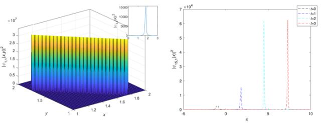
View original graphic|Download|PPT slide

Figure 1. Graphics of equation (3.23) for the values of α₁ = 0.2, γ₁ = 0.3, γ₂ = 0.5, α₂ = 0.3, λ₂ = 0.3, λ₄ = 2, S₁ = 1, and t = 1.

Here, the MATLAB symbolic package has been used to illustrate the achieved solutions using the 3D and 2D plotting displays. It can be seen that so many solutions have been derived from newly proposed extended schemes [28, 40, 41]. We have selected some of the obtained solutions and plotted their physical structures and patterns. Figure 2 depicts the physical patterns for the solution equation (3.27), which is the bright optical soliton with the values α − 1 = 0.2, γ₁ = 0.3, γ₂ = 0.2, α₂ = 0.3, λ₂ = 0.3, λ₄ = 2, S₁ = 1, and t = 1. In this case, the solution's pulse intensity is larger than the background. The background pulse invigorates as it oscillates. Nonetheless, the bright pulse diabatically retains its soliton properties, while the backdrop pulse changes. Recent experimental studies of bright-pulse propagation in fibers are very well supported by our computational results. The occurrence of a periodic orbit in solutions (3.33) and (3.37) and some other similar solutions verifies the existence of a periodic traveling wave solution. Figures 3 and 4 depict periodic wave solutions for the governing equation. Figure 5 depicts the physical patterns for the solution equation (3.72), which is the dark optical soliton with the values of α − 1 = 0.2, γ₁ = 0.3, γ₂ = 0.2, α₂ = 0.3, λ₂ = 0.3, λ₄ = 2, S₁ = 1, and t = 1. In this case, the solution's pulse intensity is smaller than the background. The background pulse weakens as it propagates, which causes a frequency chirp to occur. However, the dark pulse adiabatically retains its soliton properties, while the backdrop pulse changes. Recent experimental studies of dark-pulse propagation in fibers are very well supported by our computational results. The findings show that physical quantities and nonlinear wave qualities are linked to parameter values.

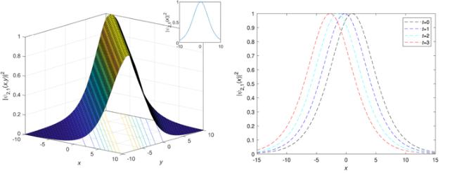
View original graphic|Download|PPT slide

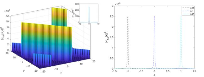
Figure 2. Graphics of equation (3.27) for the values of α₁ = 0.2, γ₁ = 0.3, γ₂ = 0.2, α₂ = 0.3, λ₂ = 0.3, λ₄ = 2, S₁ = 1, and t = 1.

View original graphic|Download|PPT slide

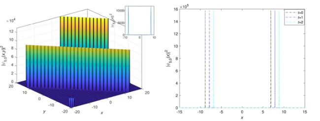
Figure 3. Graphics of equation (3.34) for the values of α₁ = 0.2, γ₁ = −0.3, γ₂ = −0.2, α₂ = −0.3, λ₂ = −0.3, λ₄ = −2, S₁ = 1, and t = 1.

View original graphic|Download|PPT slide

Figure 4. Graphics of equation (3.37) for the values of α₁ = 0.2, γ₁ = −0.3, γ₂ = −0.2, α₂ = −0.3, λ₂ = −0.3, λ₄ = −2, S₁ = 1, and t = 1.

View original graphic|Download|PPT slide

Figure 5. Graphics of equation (3.72) for the values of α₁ = 0.2, γ₁ = 0.3, γ₂ = 0.2, α₂ = 0.3, λ₂ = 0.3, λ₄ = 2, S₁ = 1, and t = 1.

5. Conclusions

In this study, using a newly proposed extended integration approach, some novel solutions for the governing equation have been constructed. Many physical elements of nonlinear models are widely acknowledged to be unknown, despite current analytical methodologies. In the anomalous dispersion, the proposed approach has been used to solve the NLSE with a higher dimension. Many intriguing solutions have been discovered. Furthermore, to throw additional light on the characteristics of the found solutions, the figures for some of the obtained solutions are graphed. The propagation properties of the developed solutions are displayed. The results reveal that the physical quantities and nonlinear wave properties are related to the parameter values. It is worth emphasizing that the new technique is extremely effective and efficient, and it has the potential to provide a plethora of creative solutions. In addition, each of the proposed results satisfied the specifications of the original issue. The findings of this study might be crucial in describing the physical characteristics of numerous nonlinear physical aspects.

Declarations

Competing interests

The authors declare that they have no conflicts of interest.

References

Publishing order | Descend order by publishing year | Descend order by cited within

1	Wazwaz A M 2020 A (2 + 1)-dimensional time-dependent Date–Jimbo–Kashiwara–Miwa equation: Painlevé integrability and multiple soliton solutions Comput. Math. Appl. 79 1145 1149 DOI

2	Wazwaz A M 2019 Multiple complex soliton solutions for integrable negative-order KdV and integrable negative-order modified KdV equations Appl. Math. Lett. 88 1 7 DOI

3	Wazwaz A M 2017 Multiple-soliton solutions for extended (3 + 1)-dimensional Jimbo–Miwa equations Appl. Math. Lett. 64 21 26 DOI

4	Wazwaz A M 2017 A two-mode modified KdV equation with multiple soliton solutions Appl. Math. Lett. 70 1 6 DOI

5	Onder I Secer A Ozisik M Bayram M 2022 On the optical soliton solutions of Kundu–Mukherjee–Naskar equation via two different analytical methods Optik 257 168761 DOI

6	Tarla S Ali K K Yilmazer R Osman M S 2022 The dynamic behaviors of the Radhakrishnan–Kundu–Lakshmanan equation by Jacobi elliptic function expansion technique Opt. Quantum Electron. 54 292

7	Tarla S Ali K K Sun T C Yilmazer R Osman M S 2022 Nonlinear pulse propagation for novel optical solitons modeled by Fokas system in monomode optical fibers Results Phys. 36 105381 DOI

8	Jaradat I Alquran M Ali M 2018 A numerical study on weak-dissipative two-mode perturbed Burgers' and Ostrovsky models: right-left moving waves Eur. Phys. J. Plus 133 164

9	Syam M Jaradat H M Alquran M 2017 A study on the two-mode coupled modified Korteweg–de Vries using the simplified bilinear and the trigonometric-function methods Nonlinear Dyn. 90 1363 1371 DOI

10	Rehman H U Ullah N Imran M A 2021 Exact solutions of Kudryashov–Sinelshchikov equation using two analytical techniques Eur. Phys. J. Plus 136 647

11	Alquran M Ali M Al-Khaled K 2012 Solitary wave solutions to shallow water waves arising in fluid dynamics Nonlinear Stud. 19 555 562

12	Alquran M Al-Khaled K Sivasundaram S Jaradat H M 2017 Mathematical and numerical study of existence of bifurcations of the generalized fractional Burgers–Huxley equation Nonlinear Stud. 24 235 244

13	Jaradat I Alquran M Momani S Biswas A 2018 Dark and singular optical solutions with dual-mode nonlinear Schrödinger's equation and Kerr-law nonlinearity Optik 172 822 825 DOI

14	Alquran M Jaradat I 2019 Multiplicative of dual-waves generated upon increasing the phase velocity parameter embedded in dual-mode Schrödinger with nonlinearity Kerr laws Nonlinear Dyn. 96 115 121 DOI

15	Sulaiman T A Yusuf A Alquran M 2021 Dynamics of optical solitons and nonautonomous complex wave solutions to the nonlinear Schrödinger equation with variable coefficients Nonlinear Dyn. 104 639 648 DOI

16	Alquran M Jaradat I Yusuf A Sulaiman T A 2021 Heart-cusp and bell-shaped-cusp optical solitons for an extended two-mode version of the complex Hirota model: application in optics Opt. Quantum Electron. 53 26

17	Alquran M 2022 New interesting optical solutions to the quadratic-cubic Schrödinger equation by using the Kudryashov-expansion method and the updated rational sine-cosine functions Opt. Quantum Electron. 54 666

18	Zhang L L Yu J P Ma W X Khalique C M Sun Y L 2021 Localized solutions of (5+ 1)-dimensional evolution equations Nonlinear Dyn. 104 4317 4327 DOI

19	Sun Y L Ma W X Yu J P 2021 N-soliton solutions and dynamic property analysis of a generalized three-component Hirota–Satsuma coupled KdV equation Appl. Math. Lett. 120 107224 DOI

20	Yu J P Sun Y L Wang F D 2020 N-soliton solutions and long-time asymptotic analysis for a generalized complex Hirota–Satsuma coupled KdV equation Appl. Math. Lett. 106 106370 DOI

21	Ali K K Yilmazer R 2022 M-lump solutions and interactions phenomena for the (2 + 1)-dimensional KdV equation with constant and time-dependent coefficients Chin. J. Phys. 77 2189 2200 DOI

22	Vitanov N K Dimitrova Z I Vitanov K N 2021 Simple Equations Method (SEsM): algorithm, connection with Hirota method, inverse scattering transform method, and several other methods Entropy 23 10

23	Ismael H F Bulut H Park C Osman M S 2020 M-lump, N-soliton solutions, and the collision phenomena for the (2 + 1)-dimensional Date–Jimbo–Kashiwara–Miwa equation Results Phys. 19 103329 DOI

24	Ismael H F Seadawy A Bulut H 2021 Rational solutions, and the interaction solutions to the (2 + 1)-dimensional time-dependent Date–Jimbo–Kashiwara–Miwa equation Int. J. Comput. Math. 98 2369 2377 DOI

25	Ali K K Seadawy A R Yokus A Yilmazer R Bulut H 2020 Propagation of dispersive wave solutions for (3 + 1)-dimensional nonlinear modified Zakharov–Kuznetsov equation in plasma physics Int. J. Mod. Phys. B 34 2050227 DOI

26	Jaradat I Alquran M Qureshi S Sulaiman T A Yusuf A 2022 Convex-rogue, half-kink, cusp-soliton and other bidirectional wave-solutions to the generalized Pochhammer–Chree equation Phys. Scr. 97 055203 DOI

27	Jaradat I Alquran M 2022 Geometric perspectives of the two-mode upgrade of a generalized Fisher–Burgers equation that governs the propagation of two simultaneously moving waves J. Comput. Appl. Math. 404 113908 DOI

28	Ali K K Yokus A Seadawy A R Yilmazer R 2022 The ion sound and Langmuir waves dynamical system via computational modified generalized exponential rational function Chaos Solitons Fractals 161 112381 DOI

29	Manafian J Ilhan O A Ismael H F Mohammed S A Mazanova S 2021 Periodic wave solutions and stability analysis for the (3 + 1)-D potential-YTSF equation arising in fluid mechanics Int. J. Comput. Math. 98 1594 1616 DOI

30	Liu Y Qin Z Chu F 2022 Investigation of magneto-electro-thermo-mechanical loads on nonlinear forced vibrations of composite cylindrical shells Commun. Nonlinear Sci. Numer. Simul. 107 106146 DOI

31	Yuan X Li L Wang Y 2019 Nonlinear dynamic soft sensor modeling with supervised long short-term memory network IEEE Trans. Industr. Inform. 16 3168 3176

32	Triki H Biswas A 2011 Dark solitons for a generalized nonlinear Schrödinger equation with parabolic law and dual power nonlinearity Math. Methods Appl. Sci. 34 958 962 DOI

33	Biswas A 2001 A perturbation of solitons due to power law nonlinearity Chaos Solitons Fractals 12 579 588 DOI

34	Suarez P Biswas A 2011 Exact 1-soliton solution of the Zakharov–Kuznetsov equation in plasmas with power law nonlinearity Appl. Math. Comput. 217 7372 7375

35	Eslami M Mirzazadeh M 2013 Topological 1-soliton of nonlinear Schrödinger equation with dual power nonlinearity in optical fibers Eur. Phys. J. Plus 128 140

36	Akinyemi L Senol M Osman M S 2022 Analytical and approximate solutions of nonlinear Schrödinger equation with higher dimension in the anomalous dispersion regime J. Ocean Eng. Sci. 7 143 154 DOI

37	Bin L Hong-Qing Z 2008 A new variable coefficient algebraic method and non-travelling wave solutions of nonlinear equations Chin. Phys. B 17 3974 DOI

38	Alquran M Jarrah A 2019 Jacobi elliptic function solutions for a two-mode KdV equation J. King Saud Univ., Sci. 31 485 489 DOI

39	Al-Ghabshi M Krishnan E Alquran M Al-Khaled K 2017 Jacobi elliptic function solutions of a nonlinear Schrödinger equation in metamaterials Nonlinear Stud. 24 469 480

40	Ismael H F Bulut H Baskonus H M Gao W 2020 Newly modified method and its application to the coupled Boussinesq equation in ocean engineering with its linear stability analysis Commun. Theor. Phys. 72 115002 DOI

41	Malik S Hashemi M S Kumar S Rezazadeh H Mahmoud W Osman M S 2023 Application of new Kudryashov method to various nonlinear partial differential equations Opt. Quantum Electron. 55 8 DOI

Options

Outlines

模态框（Modal）标题

Abstract

Cite this article

1. Introduction

2. Algorithm of new extended unified auxiliary equation method

3. Applications

3.1. Solution of equation (1.1) with the aid of case 1

4. Results and discussion

Figure 1. Graphics of equation (3.23) for the values of α1 = 0.2, γ1 = 0.3, γ2 = 0.5, α2 = 0.3, λ2 = 0.3, λ4 = 2, S1 = 1, and t = 1.

Figure 2. Graphics of equation (3.27) for the values of α1 = 0.2, γ1 = 0.3, γ2 = 0.2, α2 = 0.3, λ2 = 0.3, λ4 = 2, S1 = 1, and t = 1.

Figure 3. Graphics of equation (3.34) for the values of α1 = 0.2, γ1 = −0.3, γ2 = −0.2, α2 = −0.3, λ2 = −0.3, λ4 = −2, S1 = 1, and t = 1.

Figure 4. Graphics of equation (3.37) for the values of α1 = 0.2, γ1 = −0.3, γ2 = −0.2, α2 = −0.3, λ2 = −0.3, λ4 = −2, S1 = 1, and t = 1.

Figure 5. Graphics of equation (3.72) for the values of α1 = 0.2, γ1 = 0.3, γ2 = 0.2, α2 = 0.3, λ2 = 0.3, λ4 = 2, S1 = 1, and t = 1.

5. Conclusions

Declarations

Competing interests

References

Figure 1. Graphics of equation (3.23) for the values of α₁ = 0.2, γ₁ = 0.3, γ₂ = 0.5, α₂ = 0.3, λ₂ = 0.3, λ₄ = 2, S₁ = 1, and t = 1.

Figure 2. Graphics of equation (3.27) for the values of α₁ = 0.2, γ₁ = 0.3, γ₂ = 0.2, α₂ = 0.3, λ₂ = 0.3, λ₄ = 2, S₁ = 1, and t = 1.

Figure 3. Graphics of equation (3.34) for the values of α₁ = 0.2, γ₁ = −0.3, γ₂ = −0.2, α₂ = −0.3, λ₂ = −0.3, λ₄ = −2, S₁ = 1, and t = 1.

Figure 4. Graphics of equation (3.37) for the values of α₁ = 0.2, γ₁ = −0.3, γ₂ = −0.2, α₂ = −0.3, λ₂ = −0.3, λ₄ = −2, S₁ = 1, and t = 1.

Figure 5. Graphics of equation (3.72) for the values of α₁ = 0.2, γ₁ = 0.3, γ₂ = 0.2, α₂ = 0.3, λ₂ = 0.3, λ₄ = 2, S₁ = 1, and t = 1.