In this paper, we study the discrete Darboux and standard binary Darboux transformation for the generalized lattice Heisenberg magnet model. We calculate the quasi-Grammian solutions by the iteration of standard binary Darboux transformation. Furthermore, we derive the explicit matrix solutions for the binary Darboux matrix and then reduce them to the elementary Darboux matrix and plot the dynamics of solutions.
Zeeshan Amjad, Bushra Haider. Solitons and quasi-Grammians of the generalized lattice Heisenberg magnet model[J]. Communications in Theoretical Physics, 2023, 75(8): 085004. DOI: 10.1088/1572-9494/acda1f
1. Introduction
During the past few decades, there has been a lot of interest in the study of continuous and lattice Heisenberg magnet models. The continuous Heisenberg magnet model is completely integrable and exhibits the exact soliton solutions. Similarly, the lattice Heisenberg magnet model also preserves the integrability. The soliton solutions of this model have been studied using the inverse scattering transform, Bäcklund transformation, Darboux transformation and other solution-generating methods (see, e.g. [1–9]). The lattice Heisenberg magnet model has been studied in many works (see [10–13]). The existence of a Lax pair, Bäcklund transformation and other symmetries of the lattice Heisenberg magnet model explains many aspects of integrability [10–17]. Darboux transformation of the generalized lattice Heisenberg magnet model is studied in [25] and soliton solutions are presented.
Discrete integrable systems have received much attention from modern researchers. Many techniques, such as the Darboux transformation, the Hirota method, the Bäcklund transformation, etc, have been employed to calculate the exact solutions of many nonlinear partial differential equations ([30–36]). Binary Darboux transformation is a well-known technique used to compute the Grammian-type multisolitons of integrable systems [19, 33]. The general mechanism of this method is to keep both the spectral problem and the corresponding adjoint spectral problem associated with the nonlinear equations, which are invariant with respect to the action of the binary Darboux transformation. Furthermore, the solutions can be expressed in terms of Grammian, quasi-Grammian and quasideterminants in the literature [18, 20, 33, 37, 38].
In this paper, we study the discrete Darboux and binary Darboux transformation of the generalized lattice Heisenberg magnet (GLHM) model. For this purpose, we operate the discrete Darboux matrix on a Lax pair of GLHM models for both the direct and adjoint space to calculate the multi-soliton solutions. For the representation of solutions, we use the quasideterminant approach. Furthermore, by the iteration of binary Darboux transformation, we derive the general expressions of multi quasi-Grammian solutions. Finally, we obtain the explicit solutions for the GLHM model based upon Lie group SU(2) transformation and present the solutions, which also include the soliton solution.
where the matrix function Un ≡ Un(t) take values from Lie group ${ \mathcal G }$ in the Lie algebra g and $Psi$n ≡ $Psi$n(λ) is an N × N eigen matrix, which depends upon variable n written in subscripts defined over a lattice. The matrix function Un is subjected to constraints given by ${U}_{n}^{2}=I$ and JnUn = Un−1Jn, which also implies JnAn = An−1Jn. The compatibility condition dAn/dt + AnBn − Bn+1An = 0, is operated on (2.1), which gives the equation of motion of the GLHM model given by,
where Δnfn = fn+1 − fn. For N = 2, we have the simplest 2 × 2 case of Lie group SU(2), for which the matrix Un is expressed as ${U}_{n}={U}_{n}^{a}{\sigma }_{a}$, where σa are the familiar Pauli matrices and the constraint on the matrix Un becomes ${U}_{n}^{2}=I$. I is the 2 × 2 identity matrix. We substitute $2{\left({U}_{n}+{U}_{n-1}\right)}^{-1}=({U}_{n}+{U}_{n-1})/(1+{U}_{n}{U}_{n-1})$ in (2.6) and are able to express the equation of motion in vector notation as,
Darboux transformation is an important tool to find solutions of integrable systems represented by differential equations, partial differential equations and differential-difference equations (for details see [20–29]). We then define the Darboux transformation on the Lax pair (2.1) by using the N × N Darboux matrix Dn(λ) to calculate the soliton solutions. The Darboux matrix transforms the matrix solution from the space W to new space $\widetilde{W}$, i.e.
where I is the N × N identity matrix and Qn is the auxiliary matrix of N × N order, which is yet to be found. The choice for Qn is ${Q}_{n}={H}_{n}{{\rm{\Lambda }}}^{-1}{H}_{n}^{-1}$, where Hn is the distinct matrix solution of the Lax pair (2.1) having order N × N, which can be obtained by using i-eigenvector functions ${\rm{\Psi }}({\lambda }_{{\rm{i}}}){\left|\sigma \right\rangle }_{i}$ evaluated at λi, i = 1,…,N, whereas matrix Λ is a diagonal matrix of order N × N having eigenvalues λ1, λ2,…,λN. Therefore, matrix Hn can be defined as,,
Based upon the above results, we can prove the following theorems.
Under the action of Darboux transformation (3.5), the new solution (3.4) has the identical form as Un in equation (2.2), provided that matrix Qn fulfills the following conditions:
The relation between the Darboux transformed solution ${U}_{n}[1]$ and the untransformed solution Un is developed and defined in equation (3.10). We then have to show that the choice of matrix ${Q}_{n}={H}_{n}{{\rm{\Lambda }}}^{-1}{H}_{n}^{-1}$ satisfies the condition (3.11), i.e.
which is equivalent to (3.11). Therefore, the proof is complete.
Under the action of Darboux transformation (3.5), the new solution (3.4 ) has the identical form as Jn in equation (2.2 ), provided that matrix Qn fulfills the following conditions:
The relation between the Darboux transformed solution ${J}_{n}[1]$ and the untransformed solution Jn is developed and defined in equation (3.12). We then have to show that the choice of matrix ${Q}_{n}={H}_{n}{{\rm{\Lambda }}}^{-1}{H}_{n}^{-1}$ satisfies the condition (3.13). For this, we operate $\tfrac{{\rm{d}}}{{\rm{d}}{t}}$ on matrix $(I-{Q}_{n}^{2})$ as,
which is equivalent to (3.13). Therefore, the proof is complete.
Thus, the matrix ${Q}_{n}={H}_{n}{{\rm{\Lambda }}}^{-1}{H}_{n}^{-1}$ is a good choice, which satisfies the conditions imposed by the Darboux transformation. Thus, the Darboux transformation preserves the system, i.e. if ${{\rm{\Psi }}}_{n},{U}_{n}$ and Jn, respectively, are the solutions of the linear system (2.1) and (2.2) and the equation of motion (2.4), then ${{\rm{\Psi }}}_{n}[1],{U}_{n}[1]$ and ${W}_{n}[1]$ are also the solutions of the same equations.
In order to study the solutions we use the technique known as quasideterminants given by,
For the next iteration of Darboux transformation, take Qn,1 and Qn,2 as the two particular solutions of the Lax pair (3.3) and (3.4) at ${\rm{\Lambda }}={{\rm{\Lambda }}}_{1}^{-1}$ and ${\rm{\Lambda }}={{\rm{\Lambda }}}_{2}^{-1}$, respectively. The two-fold Darboux transformation on $Psi$n[1] is defined as,
where ${Q}_{n}[1]={H}_{n,1}{{\rm{\Lambda }}}_{1}^{-1}{H}_{n,1}^{-1}$, ${Q}_{n}[2]={H}_{n}[2]{{\rm{\Lambda }}}_{2}^{-1}{\left({H}_{n}[2]\right)}^{-1}$. Also, Hn[2] is written as,
where we have used a homological relation in the second step and a noncommutative Jacobi identity in the last step.1(1For a general quasideterminant expanded about N × N matrix D, we have $\left|\begin{array}{c}E\qquad F\qquad G\\ H\qquad A\qquad B\\ J\qquad C\qquad \boxed{D}\end{array}\right|=\left|\begin{array}{c}E\qquad G\\ J\qquad \boxed{D}\end{array}\right|-\left|\begin{array}{c}E\qquad F\\ J\qquad \boxed{C}\end{array}\right|{\left|\begin{array}{c}E\qquad F\\ H\qquad \boxed{A}\end{array}\right|}^{-1}\left|\begin{array}{c}E\qquad G\\ H\qquad \boxed{B}\end{array}\right|.$ From the noncommutative Jacobi identity, we obtain the homological relation $\left|\begin{array}{c}E\qquad F\qquad G\\ H\qquad A\qquad \boxed{B}\\ J\qquad C\qquad D\end{array}\right|=\left|\begin{array}{c}E\qquad F\qquad O\\ H\qquad A\qquad \boxed{O}\\ J\qquad C\qquad I\end{array}\right|\left|\begin{array}{c}E\qquad F\qquad G\\ H\qquad A\qquad B\\ J\qquad C\qquad \boxed{D}\end{array}\right|,$ where O and I denote the null and identity matrices, respectively.) Similarly, the K-fold Darboux transformation is given by,
The expressions given by equations (3.17) and (3.19) are the Kth solutions of the GLHM model and these results can easily be derived through induction. We then construct the adjoint Darboux transformation. The adjoint Lax pair is obtained by taking the formal adjoint of the linear equations (2.1) written as,
where η is a spectral parameter and Φn is an invertible N × N matrix field in the adjoint space W†. The Darboux matrix Dn(η) transforms the matrix solution Φn in space W† to a new matrix solution ${\tilde{{\rm{\Phi }}}}_{n}$ in $\widetilde{{W}^{\dagger }}$ i.e.
where Sn is the N × N matrix that is to be determined and I is N × N identity matrix. The covariance of the Lax pair under the Darboux transformation requires that the new solution ${\widetilde{{\rm{\Phi }}}}_{n}$ satisfies the Lax pair (3.20) given by,
By operating the Darboux transformation (3.23) on (3.24), we obtain the Darboux transformed matrix functions ${U}_{n}^{\dagger }$ and ${J}_{n}^{\dagger }$ as,
The matrix Sn can be constructed from the eigen matrices of the Lax pair and we take Sn to be ${S}_{n}={M}_{n}{{\rm{\Xi }}}^{-1}{M}_{n}^{-1}$, where Ξ= diag(η1,…,ηn) is the eigenvalue matrix. The particular matrix solution Mn of the Lax pair (3.20) is an invertible N × N matrix, which is given by,
Each column ${\left|{{\rm{\Phi }}}_{{\rm{i}}}\right\rangle }_{n}={{\rm{\Phi }}}_{n}({\eta }_{{\rm{i}}})\left|{e}_{i}\right\rangle $ in Mn is a column solution of the Lax pair (3.20). The K-fold Darboux transformation on the matrix solution and matrix function Φn, ${U}_{n}^{\dagger }$ can be written as,
Equations (3.27) and (3.28) are the Kth quasideterminant solutions of the GLHM model for the adjoint space.
4. Standard binary Darboux transformation
In order to define the binary Darboux transformation, we consider the hat space $\hat{W}$, which is a copied version of direct space W, so the corresponding solutions are ${\hat{{\rm{\Phi }}}}_{n}$ ∈$\hat{W}$. Therefore, the equation of motion and the compatibility condition will have the identical form as that for the direct space given by,
The specific solutions for the direct and adjoint spaces are Hn and Sn, respectively. Thus, the corresponding solutions for $\hat{W}$ are ${\hat{H}}_{n}$ ∈$\hat{W}$ and ${\hat{{\rm{\Phi }}}}_{n}$ ∈ ${\hat{W}}_{n}^{\dagger }.$ Also assuming that ${\rm{i}}({\hat{H}}_{n})$ ∈ ${\widetilde{W}}^{\dagger },$ we can then write the transformation as,
Also from ${D}_{n}^{\dagger }(\lambda )({\rm{i}}({H}_{n}))=0$, we obtain ${\rm{i}}({H}_{n})={M}_{n}^{(-1)\dagger }$ and similarly ${\rm{i}}({\hat{M}}_{n})={\hat{M}}_{n}^{(-1)\dagger }$. Therefore, from the above equations we can write,
where ${D}_{n}(\lambda )={\lambda }^{-1}I-{H}_{n}{{\rm{\Lambda }}}^{-1}{H}_{n}^{-1}$. By substituting the expression of Dn(λ) in equation (4.5), we obtain,
Therefore, the required potential is expressed in terms of particular matrix solutions to the Lax pair as well as to the adjoint Lax pair of the GLHM model. We then define the Darboux matrix in hat space:
This expression can be further simplified when we introduce potential Δn instead of matrices in the hat space. By using equation (4.6), the above equation becomes,
Similarly, using the iteration process we can calculate the quasideterminant solutions for ${U}_{n}^{\dagger }$.
Therefore, we can calculate the Grammian-type solutions for the GLHM model by using standard binary Darboux transformation. In addition, the potential can be expressed in the form of quasideterminants. Thus, by developing the binary Darboux transformation in terms of spectral parameters, we can obtain expressions of matrix solutions in the form of Grammian-type quasideterminants that have a different form as calculated using elementary Darboux transformation.
5. Explicit solutions
In this section, we consider the GLHM model based on the Lie group SU(2) and obtain the soliton solutions by using the binary Darboux transformation. To obtain an explicit expression for the soliton solution in the general N × N case, we take the seed solution,
are respectively p × p and (N − p) × (N − p) matrices. Here, n in the subscript is a discrete index. We then take the seed solution for the case N = 2, which is given as,
The expression for ${Q}_{n}={H}_{n}{{\rm{\Lambda }}}^{-1}{H}_{n}^{-1}$ by using ${\rm{\Lambda }}=\left(\begin{array}{cc}\lambda & 0\\ 0 & \bar{\lambda }\end{array}\right)$ becomes,
In order to obtain the expression for ${\hat{U}}_{n}$, we start from the definition of Δn(Hn, Mn) given in (4.11) and by using (5.4), (5.7), we obtain,
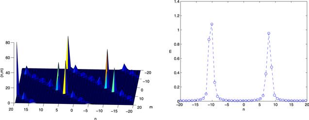
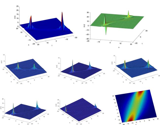
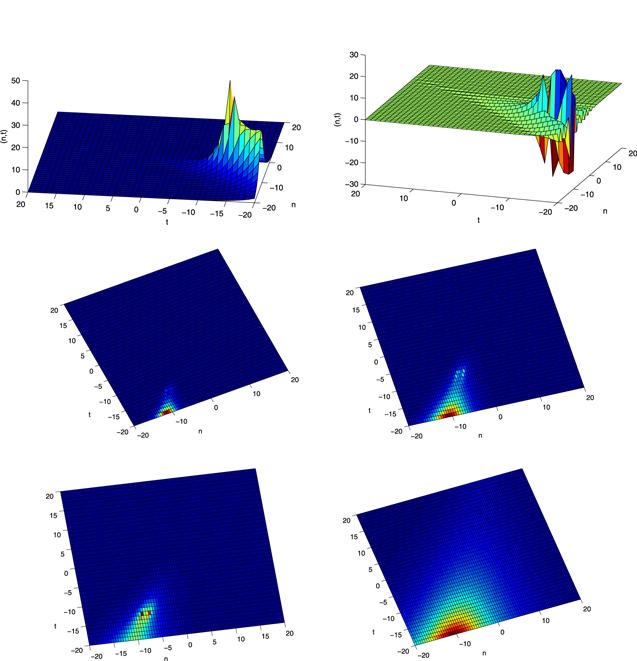
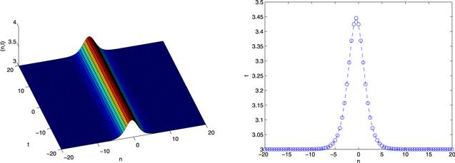
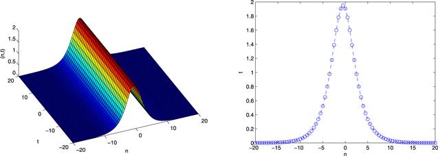
From (5.15), it can be seen that U†[1] = − U[1] and Tr(U[1]) =0. Therefore, it can be said that the above expression (5.15) is an explicit equation based on SU(2) one-soliton solutions of the GLHM model.
We can obtain solutions in the form of direct and adjoint space parameters, by using the standard binary Darboux transformation, which are different to those obtained by elementary Darboux transformation. In addition, we reduce the solutions into the elementary Darboux transformation solutions, which is the advantage of binary Darboux transformation.
6. Conclusion
In this paper, we have composed the discrete Darboux transformation of the GLHM model not only for the direct space, but also for the adjoint space, and also calculated the standard binary Darboux transformation of the model. By iterating the standard binary Darboux transformation we have obtained the multi-Grammian solutions in terms of quasideterminants. We have calculated the explicit solutions for the Grammian solutions of the model. We presented the dynamics of the solutions and by reducing the solutions also obtain the one-soliton solution for the semi-discrete model. This work can be extended in various interesting directions. For example, one can study discrete and semi-discrete versions of the multi-component GLHM model as well as their multi-soliton solutions. It would also be interesting to study discrete rogue and hump wave solutions for the GLHM model.
Declaration of competing interests
The authors declare that they have no known competing financial interests or personal relationships that could have appeared to influence the work reported in this paper.
CienskiJ LCzarneckaJ2006 The Darboux–Bäcklund transformation for the static 2-dimensional continuum Heisenberg chain J. Phys. A: Math. Gen.39 11003 11012
FaddeevL D1984 Integrable models in (1+1)-dimensional quantum field theory Recent Advances in Field Theory and Statistical Mechanics (Les Houches, 2 August–10 September 1982ZuberJ-BStoraR Amsterdam North-Holland 561 608
11
SklyaninE K1982 Some algebraic structures connected with the Yang–Baxter equation Funct. Anal. Appl.16 263 270
HaldaneF D M1982 Excitation spectrum of a generalized Heisenberg ferromagnet spin chain with arbitrary spin J. Phys. C: Solid State Phys.15 L1309–L1313
HaldaneF D M1986 Geometrical interpretation of momentum and crystal momentum of classical and quantum ferromagnetic Heisenberg chains Phys. Rev. Lett.57 1488 1491
TsuchidaT2010 A systematic method for constructing time discretizations of integrable lattice systems: local equations of motion J. Phys. A: Math. Theor.43 415202
MatveevV BSalleM A1991Darboux Transformations and Solitons Berlin Springer Press
23
GuC HHuH SZhouZ X2005Darboux Transformation in Soliton Theory and Its Geometric Applications Shanghai Shanghai Scientific and Technical Publishers
24
ZhangH QTianBLiJXuTZhangY X2009 Symbolic-computation study of integrable properties for the (2 +1)-dimensional Gardner equation with the two-singular manifold method IMA J. Appl. Math.74 46
ShiYNimmoJ J CZhangD2014 Darboux and binary Darboux transformations for discrete integrable systems I. Discrete potential KdV equation J. Phys. A: Math. Theor.47 025205


