Welcome to visit Communications in Theoretical Physics,
Mathematical Physics

Chirped optical solitons and stability analysis of the nonlinear Schrödinger equation with nonlinear chromatic dispersion

  • Thilagarajah Mathanaranjan 1 ,
  • Mir Sajjad Hashemi 2 ,
  • Hadi Rezazadeh 3 ,
  • Lanre Akinyemi 4 ,
  • Ahmet Bekir , 5,
Expand
  • 1Department of Mathematics and Statistics, University of Jaffna, Sri Lanka
  • 2Department of Computer Engineering, Biruni University, 34010 Istanbul, Turkey
  • 3Faculty of Engineering Technology, Amol University of Special Modern Technologies, Amol, Iran
  • 4Department of Mathematics, Lafayette College, Easton, PA, United States of America
  • 5Neighborhood of Akcaglan, Imarli Street, Number: 28/4, 26030, Eskisehir, Turkey

Author to whom any correspondence should be addressed.

Received date: 2023-03-13

  Revised date: 2023-07-04

  Accepted date: 2023-07-04

  Online published: 2023-07-31

Copyright

© 2023 Institute of Theoretical Physics CAS, Chinese Physical Society and IOP Publishing

Abstract

The present paper aims to investigate the chirped optical soliton solutions of the nonlinear Schrödinger equation with nonlinear chromatic dispersion and quadratic-cubic law of refractive index. The exquisite balance between the chromatic dispersion and the nonlinearity associated with the refractive index of a fiber gives rise to optical solitons, which can travel down the fiber for intercontinental distances. The effective technique, namely, the new extended auxiliary equation method is implemented as a solution method. Different types of chirped soliton solutions including dark, bright, singular and periodic soliton solutions are extracted from the Jacobi elliptic function solutions when the modulus of the Jacobi elliptic function approaches to one or zero. These obtained chirped optical soliton solutions might play an important role in optical communication links and optical signal processing systems. The stability of the system is examined in the framework of modulational instability analysis.

Cite this article

Thilagarajah Mathanaranjan , Mir Sajjad Hashemi , Hadi Rezazadeh , Lanre Akinyemi , Ahmet Bekir . Chirped optical solitons and stability analysis of the nonlinear Schrödinger equation with nonlinear chromatic dispersion[J]. Communications in Theoretical Physics, 2023 , 75(8) : 085005 . DOI: 10.1088/1572-9494/ace3b0

1. Introduction

In nonlinear sciences, the study of accurate solutions to nonlinear partial differential equations (NLPDEs) is important because physical processes in the real world may be efficiently described by applying the theory of mathematical tools [1, 2]. NLPDEs have had a significant impact on applied science and engineering over the last two decades [3, 4]. The study of the soliton solutions explores a theoretical reference for the research of nonlinear physical models, soliton control, optical switching equipment and so on. Up to now, many effective and powerful methods have been obtained for constructing the soliton solutions of the NLPDEs, such as the soliton ansatz method [5, 6], the Kudryashov method [7], the Hirota's bilinear transform method [8, 9], the Darboux transformation method [10, 11], the extended trial equation method [12], the Lie symmetry method [13, 14], the improved F-expansion approach [15], the invariant subspace method [16, 17], the extended sinh-Gordon equation expansion method [18] and the new extended auxiliary equation method [19, 20], the $({G}^{{\prime} }/G)$-expansion method [2123], the Exp-function method [24, 25], the modified simplest equation method [26, 27], the decomposition method [28, 29], and so on.
The exquisite balance between the chromatic dispersion (CD) and the nonlinearity associated with the refractive index of a fiber gives rise to optical solitons, which can travel down the fiber for intercontinental distances. For an instant, consider the NLSE with nonlinear CD and quadratic-cubic (QC) law of refractive index of the form [30]
$\begin{eqnarray}{\rm{i}}{q}_{t}+a{\left(| q{| }^{n}q\right)}_{\mathrm{xx}}+\left({b}_{1}| q| +{b}_{2}| q{| }^{2}\right)q=0,\end{eqnarray}$
where a is the coefficient of nonlinear CD while b1 and b2 stand for self-phase modulation that describes the nonlinear structure of the fiber refractive index. The considered model identifies the soliton pulse propagation in the optical fibers. The stationary optical solitons for this model have been derived in [30] using direct substitution and the results are obtained in the form of Appell's hypergeometric functions. The aim of this paper is mainly to derive various chirped optical soliton solutions of the model by means of the new extended auxiliary equation (NEAE) method. The NEAE method is an effective and straightforward mathematical tool for constructing the exact solutions of NLPDEs and gained considerable attention in recent years.
The remaining part of the paper is arranged as follows. Section 2 is dedicated to briefly explaining the NEAE method. In section 3, we presented the governing model in detail. We employed the NEAE method to a governing model and chirped solitons are obtained in section 4. We have also applied the linear stability analysis in section 5. The physical interpretations and concluding remarks are given in sections 6 and 7 respectively.

2. The essences of proposed method

In this section, we give a brief introduction to the NEAE method [19, 20]. Consider the following nonlinear PDE:
$\begin{eqnarray}H\left(q,{q}_{x},{q}_{t},{q}_{{xx}},{q}_{{tt}}\right)=0,\end{eqnarray}$
where H is a polynomial function in q. The main steps of the NEAE method are given as follows:
Step 1. Applying the following transformation
$\begin{eqnarray}q(x,t)=q(\zeta ),\,\,\,\,\,\,\zeta =k(x-\omega t),\end{eqnarray}$
where k and ω are constants. Inserting equation (3) into equation (2), the following ODE is obtained:
$\begin{eqnarray}G(q,{q}^{{\prime} },{q}^{{\prime\prime} },\ldots )=0.\end{eqnarray}$
Step 2. Let the solution q(ζ) of equation (4) is
$\begin{eqnarray}q(\zeta )=\displaystyle \sum _{i=0}^{2N}{a}_{i}{G}^{i}(\zeta ),\end{eqnarray}$
and G(ζ) satisfies the following ODE:
$\begin{eqnarray}{\left({G}^{{\prime} }(\zeta )\right)}^{2}={c}_{0}+{c}_{2}{G}^{2}(\zeta )+{c}_{4}{G}^{4}(\zeta )+{c}_{6}{G}^{6}(\zeta ),\end{eqnarray}$
here ai(i = 0, …...2N) and cj(j = 0, 2, 4, 6) are the coefficients to be determined later.
Step 3. N in equation (5) is a positive integer which is obtained from the homogenous balance principle of q(ζ) in equation (4).
Step 4. We insert (5) and (6) in equation (4), then equating the coefficients of power of ${G}^{j}{({G}^{{\prime} })}^{l}(j=0,1,2...)$ and (l = 0, 1) to zero generates a system of the algebraic equation systems for cj(j = 0, 2, 4, 6), ai(i = 0, …..2N), k and ω. , which can be evaluated by Maple or Mathematica.
Step 6. The equation (6) has the following solutions:
$\begin{eqnarray}G\left(\zeta \right)=\displaystyle \frac{1}{2}{\left[-\displaystyle \frac{{c}_{4}}{{c}_{6}}\left(1\pm g(\zeta )\right)\right]}^{\tfrac{1}{2}},\end{eqnarray}$
where the function g(ζ) could be explained using the Jacobi elliptic functions (JEFs) $\mathrm{sn}(\zeta ,m)$, $\mathrm{cn}(\zeta ,m)$, $\mathrm{dn}(\zeta ,m)$ and so on, where m is the modulus of the JEFs. When m tends to 1 or 0, JEFs reduce to trigonometric and hyperbolic functions.
The functions g(ζ) given in (7) have twelve type solutions as follows:
1.

1.If ${c}_{0}=\tfrac{{c}_{4}^{3}\,\left({m}^{2}-1\right)}{32{c}_{6}^{2}{m}^{2}}\,,\,\,\,{c}_{2}=\tfrac{{c}_{4}^{2}\left(5{m}^{2}-1\right)}{16{c}_{6}{m}^{2}},\,\,\,\,{c}_{6}\gt 0,$ then

$\begin{eqnarray}g(\zeta )=\mathrm{sn}(\rho \zeta )\,\,\,\,\,\mathrm{or}\,\,\,\,\,g(\zeta )=\displaystyle \frac{1}{m\,\mathrm{sn}(\rho \zeta ))},\end{eqnarray}$
where $\rho =\tfrac{{c}_{4}}{2m}\sqrt{\tfrac{1}{{c}_{6}}}$.

2.

2.If ${c}_{0}=\tfrac{{c}_{4}^{3}\,(1-{m}^{2})}{32{c}_{6}^{2}}\,,\,\,\,{c}_{2}=\tfrac{{c}_{4}^{2}\left(5-{m}^{2}\right)}{16{c}_{6}},\,\,\,\,{c}_{6}\gt 0,$ then

$\begin{eqnarray}g(\zeta )=m\,\mathrm{sn}(\rho \zeta )\,\,\,\,\,\mathrm{or}\,\,\,\,\,g(\zeta )=\displaystyle \frac{1}{\mathrm{sn}(\rho \zeta ))},\end{eqnarray}$
where $\rho =\tfrac{{c}_{4}}{2}\sqrt{\tfrac{1}{{c}_{6}}}.$

3.

3.If ${c}_{0}=\tfrac{{c}_{4}^{3}}{32{m}^{2}{c}_{6}^{2}}\,,\,\,\,{c}_{2}=\tfrac{{c}_{4}^{2}\left(4{m}^{2}+1\right)}{16{c}_{6}{m}^{2}},\,\,\,\,{c}_{6}\lt 0,$ then

$\begin{eqnarray}g(\zeta )=\mathrm{cn}(\rho \zeta )\,\,\,\,\,\mathrm{or}\,\,\,\,\,g(\zeta )=\displaystyle \frac{\sqrt{1-{m}^{2}}\,\mathrm{sn}(\rho \zeta )}{\mathrm{dn}(\rho \zeta ))},\end{eqnarray}$
where $\rho =\tfrac{-{c}_{4}}{2m}\sqrt{\tfrac{-1}{{c}_{6}}}.$

4.

4.If ${c}_{0}=\tfrac{{c}_{4}^{3}{m}^{2}}{32{c}_{6}^{2}({m}^{2}-1)},\,\,\,{c}_{2}=\tfrac{{c}_{4}^{3}\left(5{m}^{2}-4\right)}{16{c}_{6}({m}^{2}-1)},\,\,\,{c}_{6}\lt 0,$ then

$\begin{eqnarray}g(\zeta )=\displaystyle \frac{\mathrm{dn}\left(\rho \zeta \right)}{\sqrt{1-{m}^{2}}}\,\,\,\,\,\mathrm{or}\,\,\,\,\,g(\zeta )=\displaystyle \frac{1}{\mathrm{dn}(\rho \zeta ))}\,,\end{eqnarray}$
where $\rho =\tfrac{{c}_{4}}{2}\sqrt{\tfrac{1}{{c}_{6}\,({m}^{2}-1)}}\,.$

5.

5.If ${c}_{0}=\tfrac{{c}_{4}^{3}}{32{c}_{6}^{2}(1-{m}^{2})}\,,\,\,\,{c}_{2}=\tfrac{{c}_{4}^{2}\left(4{m}^{2}-5\right)}{16{c}_{6}({m}^{2}-1)},\,\,\,\,{c}_{6}\gt 0,$ then

$\begin{eqnarray}g(\zeta )=\displaystyle \frac{1}{\mathrm{cn}(\zeta \rho )}\,\,\,\,\,\mathrm{or}\,\,\,\,\,g(\zeta )=\displaystyle \frac{\mathrm{dn}(\zeta \rho )}{\sqrt{1-{m}^{2}}\,\mathrm{sn}\left(\rho \zeta \right)}\,,\end{eqnarray}$
where $\rho =\tfrac{{c}_{4}}{2}\sqrt{\tfrac{1}{{c}_{6}\,(1-{m}^{2})}}$.

6.

6.If ${c}_{0}=\tfrac{{m}^{2}{c}_{4}^{3}}{32{c}_{6}^{2}},\,\,\,{c}_{2}=\tfrac{{c}_{4}^{2}\left({m}^{2}+4\right)}{16{c}_{6}},\,\,\,\,{c}_{6}\lt 0,$ then

$\begin{eqnarray}g(\zeta )=\mathrm{dn}(\rho \zeta )\,\,\,\,\,\mathrm{or}\,\,\,\,\,g(\zeta )=\displaystyle \frac{\sqrt{1-{m}^{2}}}{\mathrm{dn}\left(\rho \zeta \right)}\,,\end{eqnarray}$
where $\rho =\tfrac{-{c}_{4}}{2}\sqrt{\tfrac{-1}{{c}_{6}\,}}$.

Step 7. Finally, we insert the values cj, ai, k, ω and the solutions (8)–(13) into (5) to get the JEFs of equation (1)

3. Mathematical analysis of the model

Assume that the complex wave function q(x, t) of equation (1) can be taken as follows [31]:
$\begin{eqnarray}q(x,t)=\phi (\zeta ){{\rm{e}}}^{{\rm{i}}(\psi (\zeta )+\omega t)},\,\,\,\,\,\,\zeta =x-\tau t,\end{eqnarray}$
here ψ and φ are the real functions. Also, τ and ω represent the soliton velocity and the frequency respectively. The corresponding chirp is given as follows [31]:
$\begin{eqnarray}\delta \omega (x,t)=-\displaystyle \frac{\partial }{\partial x}[\psi (\zeta )+\omega t]=-\psi ^{\prime} (\zeta ).\end{eqnarray}$
Now, inserting equation (14) into equation (1), and collecting the real and imaginary parts yields
$\begin{eqnarray}\begin{array}{l}-\omega \phi {\left(\zeta \right)}^{2}+{b}_{1}\phi {\left(\zeta \right)}^{3}+{b}_{2}\phi {\left(\zeta \right)}^{4}+\tau \phi {\left(\zeta \right)}^{2}\psi ^{\prime} (\zeta )\\ +{an}(1+n)\phi {\left(\zeta \right)}^{n}\phi ^{\prime} {\left(\zeta \right)}^{2}-a\phi {\left(\zeta \right)}^{2+n}\psi ^{\prime} {\left(\zeta \right)}^{2}\\ +a(1+n)\phi {\left(\zeta \right)}^{1+n}\phi ^{\prime\prime} (\zeta )=0,\end{array}\end{eqnarray}$
$\begin{eqnarray}-\tau \phi ^{\prime} (\zeta )+2a(1+n)\phi {\left(\zeta \right)}^{n}\phi ^{\prime} (\zeta )\psi ^{\prime} (\zeta )+a\phi {\left(\zeta \right)}^{1+n}\psi ^{\prime\prime} (\zeta )=0.\end{eqnarray}$
We set the chirp as
$\begin{eqnarray}\psi ^{\prime} (\zeta )=A\phi {\left(\zeta \right)}^{-n}+B,\end{eqnarray}$
where A is the nonlinear chirp parameter and B is the constant chirp parameter. Accordingly, the resultant chirp takes the form
$\begin{eqnarray}\delta \omega (x,t)=-(A\phi {\left(\zeta \right)}^{-n}+B).\end{eqnarray}$
Substituting equation (18) into equation (17) yields after some algebra
$\begin{eqnarray}A=\displaystyle \frac{\tau }{a(2+n)}\,\,\,\,\mathrm{and}\,\,\,\,B=0.\end{eqnarray}$
Now substituting the equation (20) to equation (18) and replacing in equation (16) yields,
$\begin{eqnarray}-\omega \phi {\left(\zeta \right)}^{2}+{b}_{1}\phi {\left(\zeta \right)}^{3}+{b}_{2}\phi {\left(\zeta \right)}^{4}+\frac{{\tau }^{2}(1\,+\,n)}{a(2\,+\,n{)}^{2}}\phi {\left(\zeta \right)}^{2-n}+{an}(1+n)\phi {\left(\zeta \right)}^{n}\phi ^{\prime} {\left(\zeta \right)}^{2}+a(1+n)\phi {\left(\zeta \right)}^{1+n}\phi ^{\prime\prime} (\zeta )=0.\end{eqnarray}$
In the following section, we will solve equation (21) by using the suggested method.

4. Chirped soliton solution

This section is to apply the NEAE method to find the chirped soliton solutions of equation (1).
In order to receive the integration of equation (21) it is essential to prefer n = 1. Assuming n = 1, equation (21) reduce to
$\begin{eqnarray}\begin{array}{l}2{\tau }^{2}-9a\omega \phi (\zeta )+9{{ab}}_{1}\phi {\left(\zeta \right)}^{2}+9{{ab}}_{2}\phi {\left(\zeta \right)}^{3}+18{a}^{2}\phi ^{\prime} {\left(\zeta \right)}^{2}\\ +18{a}^{2}\phi (\zeta )\phi ^{\prime\prime} (\zeta )=0.\end{array}\end{eqnarray}$
Balancing the φ(ζ)φ″(ζ) and $\phi {\left(\zeta \right)}^{3}$ in (22), yields N = 2. In accordance with the NEAE method [19, 20], we suppose that equation (22) has the following form:
$\begin{eqnarray}\phi (\zeta )={\alpha }_{0}+{\alpha }_{1}G(\zeta )+{\alpha }_{2}G{\left(\zeta \right)}^{2}+{\alpha }_{3}G{\left(\zeta \right)}^{3}+{\alpha }_{4}G{\left(\zeta \right)}^{4},\end{eqnarray}$
while the G(ζ) satisfies the following ODE:
$\begin{eqnarray}{\left({G}^{{\prime} }(\zeta )\right)}^{2}={c}_{0}+{c}_{2}{G}^{2}(\zeta )+{c}_{4}{G}^{4}(\zeta )+{c}_{6}{G}^{6}(\zeta ).\end{eqnarray}$
Substituting equation (23) along with equation (24) into (22), correlating the coefficients of powers of Gi(i = 0, 1, 2, …., 8) to zero, generates a system of the algebraic equation. By solving the system of equations, we get
$\begin{eqnarray}\begin{array}{l}{\alpha }_{1}={\alpha }_{3}=0,\,{c}_{0}=\displaystyle \frac{{\alpha }_{2}\left(-5{b}_{1}{\alpha }_{4}+{b}_{2}\left({\alpha }_{2}^{2}-12{\alpha }_{0}{\alpha }_{4}\right)\right)}{320a{\alpha }_{4}^{2}},\\ {c}_{2}=-\displaystyle \frac{5{b}_{1}{\alpha }_{4}+3{b}_{2}\left({\alpha }_{2}^{2}+4{\alpha }_{0}{\alpha }_{4}\right)}{320a{\alpha }_{4}},\\ {c}_{4}=-\displaystyle \frac{{b}_{2}{\alpha }_{2}}{40a},\,{c}_{6}=-\displaystyle \frac{{b}_{2}{\alpha }_{4}}{80a},\\ \omega =\displaystyle \frac{3\left(5{b}_{1}{\alpha }_{4}\left(-{\alpha }_{2}^{2}+8{\alpha }_{0}{\alpha }_{4}\right)+{b}_{2}\left({\alpha }_{2}^{4}-12{\alpha }_{0}{\alpha }_{2}^{2}{\alpha }_{4}+48{\alpha }_{0}^{2}{\alpha }_{4}^{2}\right)\right)}{80{\alpha }_{4}^{2}},\\ \tau =\pm \displaystyle \frac{3}{4{\alpha }_{4}}\sqrt{\displaystyle \frac{a{\alpha }_{0}\left(-{\alpha }_{2}^{2}+4{\alpha }_{0}{\alpha }_{4}\right)\left(5{b}_{1}{\alpha }_{4}-{b}_{2}\left({\alpha }_{2}^{2}-8{\alpha }_{0}{\alpha }_{4}\right)\right)}{5}},\end{array}\end{eqnarray}$
provided that $\left[a{\alpha }_{0}\left(-{\alpha }_{2}^{2}+4{\alpha }_{0}{\alpha }_{4}\right)\left(5{b}_{1}{\alpha }_{4}-{b}_{2}\left({\alpha }_{2}^{2}-8{\alpha }_{0}{\alpha }_{4}\right)\right)\right]\gt 0$. Inserting equation (25) into equation (23) along with equation (7), we have the following JEF of equation (22):
$\begin{eqnarray}\phi (\zeta )={\alpha }_{0}+\displaystyle \frac{{\alpha }_{2}^{2}}{4{\alpha }_{4}}\left[-1+g{\left(\zeta \right)}^{2}\right],\end{eqnarray}$
where g(ζ) has the forms (8)-(13), respectively. According to forms (8)–(13), equation (1) has the following types of solutions from (26) and (14):
Type 1. If ${c}_{0}=\tfrac{{c}_{4}^{3}\,\left({m}^{2}-1\right)}{32{c}_{6}^{2}{m}^{2}},\,{c}_{2}=\tfrac{{c}_{4}^{2}\left(5{m}^{2}-1\right)}{16{c}_{6}{m}^{2}},\,{c}_{6}\gt 0,$ then the JEFs solutions of equation (1) as:
$\begin{eqnarray}\begin{array}{l}q(x,t)=\displaystyle \frac{1}{12}\left[-\displaystyle \frac{5{b}_{1}}{{b}_{2}}+\displaystyle \frac{{\alpha }_{2}^{2}}{{\alpha }_{4}}\left(-1-\displaystyle \frac{1}{{m}^{2}}\right.\right.\\ \left.\left.+3\,{\mathrm{sn}}^{2}\left(-\displaystyle \frac{{\alpha }_{2}}{4m}\sqrt{-\displaystyle \frac{{b}_{2}}{5a{\alpha }_{4}}}\,\zeta \right)\right)\right]{{\rm{e}}}^{{\rm{i}}(\psi (\zeta )+\omega t)},\end{array}\end{eqnarray}$
or
$\begin{eqnarray}\begin{array}{l}q(x,t)=\displaystyle \frac{1}{12}\left[-\displaystyle \frac{5{b}_{1}}{{b}_{2}}+\displaystyle \frac{{\alpha }_{2}^{2}}{{\alpha }_{4}}\left(-1-\displaystyle \frac{1}{{m}^{2}}\right.\right.\\ \left.\left.+\displaystyle \frac{3}{{m}^{2}{\mathrm{sn}}^{2}\left(-\tfrac{{\alpha }_{2}}{4m}\sqrt{-\tfrac{{b}_{2}}{5a{\alpha }_{4}}}\,\zeta \right)}\right)\right]{{\rm{e}}}^{{\rm{i}}(\psi (\zeta )+\omega t)},\end{array}\end{eqnarray}$
with ab2α4 < 0. If m tends to 1, then $\mathrm{sn}(\zeta )$ tends to $\tanh (\zeta )$, and on account of this, we acquire the dark soliton solutions:
$\begin{eqnarray}q(x,t)=\displaystyle \frac{1}{12}\left[-\displaystyle \frac{5{b}_{1}}{{b}_{2}}+\displaystyle \frac{{\alpha }_{2}^{2}}{{\alpha }_{4}}\left(-2+3\,{\tanh }^{2}\left(-\displaystyle \frac{{\alpha }_{2}}{4}\sqrt{-\displaystyle \frac{{b}_{2}}{5a{\alpha }_{4}}}\,\zeta \right)\right)\right]{{\rm{e}}}^{{\rm{i}}(\psi (\zeta )+\omega t)},\end{eqnarray}$
and the singular soliton solutions:
$\begin{eqnarray}q(x,t)=\displaystyle \frac{1}{12}\left[-\displaystyle \frac{5{b}_{1}}{{b}_{2}}+\displaystyle \frac{{\alpha }_{2}^{2}}{{\alpha }_{4}}\left(-2+3\,{\coth }^{2}\left(-\displaystyle \frac{{\alpha }_{2}}{4}\sqrt{-\displaystyle \frac{{b}_{2}}{5a{\alpha }_{4}}}\zeta \right)\right)\right]{{\rm{e}}}^{{\rm{i}}(\psi (\zeta )+\omega t)}.\end{eqnarray}$
The dynamical behaviors of solutions (29) and (30) are presented in figures 1 and 2.
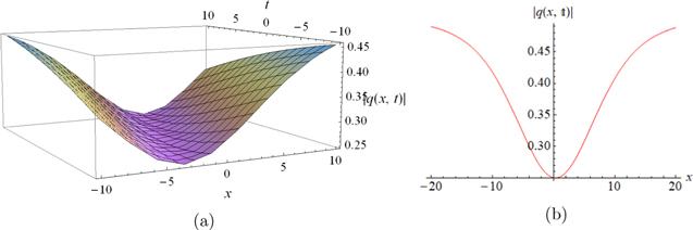
Figure 1. (a) 3D profile of solution (29) with m = a = b1 = b2 = α2 = 1, α4 = −1, k = ω = 1 (b) 2D curve for t = 1.
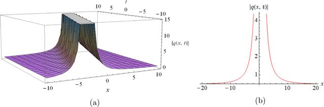
Figure 2. (a) 3D profile of solution (30) with m = a = b1 = b2 = α2 = 1, α4 = −1, k = ω = 1 (b) 2D curve for t = 1.
Type 2. If ${c}_{0}=\tfrac{{c}_{4}^{3}\left(1-{m}^{2}\right)}{32{c}_{6}^{2}},\,{c}_{2}=\tfrac{{c}_{4}^{2}\left(5-{m}^{2}\right)}{16{c}_{6}},\,{c}_{6}\gt 0,$ then the JEFs solutions of equation (1) as:
$\begin{eqnarray}\begin{array}{l}q(x,t)=\displaystyle \frac{1}{12}\left[-\displaystyle \frac{5{b}_{1}}{{b}_{2}}+\displaystyle \frac{{\alpha }_{2}^{2}}{{\alpha }_{4}}\left(\Space{0ex}{3.05ex}{0ex}-1-{m}^{2}\right.\right.\\ \left.\left.+3{m}^{2}{\mathrm{sn}}^{2}\left(\displaystyle \frac{{\alpha }_{2}}{4}\sqrt{-\displaystyle \frac{{b}_{2}}{5a{\alpha }_{4}}}\,\zeta \right)\right)\right]{{\rm{e}}}^{{\rm{i}}(\psi (\zeta )+\omega t)},\end{array}\end{eqnarray}$
or
$\begin{eqnarray}\begin{array}{l}q(x,t)=\displaystyle \frac{1}{12}\left[-\displaystyle \frac{5{b}_{1}}{{b}_{2}}+\displaystyle \frac{{\alpha }_{2}^{2}}{{\alpha }_{4}}\left(\Space{0ex}{5.05ex}{0ex}-1-{m}^{2}\right.\right.\\ \left.\left.+\displaystyle \frac{3}{{\mathrm{sn}}^{2}\left(\tfrac{{\alpha }_{2}}{4}\sqrt{-\tfrac{{b}_{2}}{5a{\alpha }_{4}}}\,\zeta \right)}\right)\right]{{\rm{e}}}^{{\rm{i}}(\psi (\zeta )+\omega t)},\end{array}\end{eqnarray}$
with ab2α4 < 0. If m tends to 0, then $\mathrm{sn}(\zeta )$ tends to $\sin (\zeta )$, and on account of this from solution (32), we acquire the singular periodic wave solution
$\begin{eqnarray}\begin{array}{l}q(x,t)=\displaystyle \frac{1}{12}\left[-\displaystyle \frac{5{b}_{1}}{{b}_{2}}+\displaystyle \frac{{\alpha }_{2}^{2}}{{\alpha }_{4}}\right.\\ \left.\times \left(-1+3\,{\csc }^{2}\left(\displaystyle \frac{{\alpha }_{2}}{4}\sqrt{-\displaystyle \frac{{b}_{2}}{5a{\alpha }_{4}}}\,\zeta \right)\right)\right]{{\rm{e}}}^{{\rm{i}}(\psi (\zeta )+\omega t)}.\end{array}\end{eqnarray}$
If m tends to 1, then $\mathrm{sn}(\zeta )$ tends to $\tanh (\zeta )$, and hence from solution (31) and (32) we recover solutions (29) and (30), respectively.
The dynamical behaviors of solution (33) are presented in figure 3.
Figure 3. (a) 3D profile of the solution (33) with m = a = b1 = b2 = α2 = 1, α4 = −1, k = ω = 1 (b) 2D curve for t = 1.
Type 3. If ${c}_{0}=\tfrac{{c}_{4}^{3}}{32{c}_{6}^{2}{m}^{2}},\,{c}_{2}=\tfrac{{c}_{4}^{2}\left(4{m}^{2}+1\right)}{16{c}_{6}{m}^{2}},\,{c}_{6}\lt 0,$ then the JEFs solutions of equation (1) as:
$\begin{eqnarray}\begin{array}{l}q(x,t)=\displaystyle \frac{1}{12}\left[-\displaystyle \frac{5{b}_{1}}{{b}_{2}}+\displaystyle \frac{{\alpha }_{2}^{2}}{{m}^{2}{\alpha }_{4}}\left(1-2{m}^{2}\right.\right.\\ \left.\left.+3{m}^{2}{\mathrm{cn}}^{2}\left(\displaystyle \frac{{\alpha }_{2}}{4m}\sqrt{\displaystyle \frac{{b}_{2}}{5a{\alpha }_{4}}}\,\zeta \right)\right)\right]{{\rm{e}}}^{{\rm{i}}(\psi (\zeta )+\omega t)},\end{array}\end{eqnarray}$
or
$\begin{eqnarray}\begin{array}{l}q(x,t)=\displaystyle \frac{1}{12}\left[-\displaystyle \frac{5{b}_{1}}{{b}_{2}}+\displaystyle \frac{{\alpha }_{2}^{2}}{{m}^{2}{\alpha }_{4}}\left(\left(1-2{m}^{2}\right)\right.\right.\\ \left.\left.-3{m}^{2}\left(-1+{m}^{2}\right)\displaystyle \frac{{\mathrm{sn}}^{2}\left(\tfrac{{\alpha }_{2}}{4m}\sqrt{\tfrac{{b}_{2}}{5a{\alpha }_{4}}}\,\zeta \right)}{{\mathrm{dn}}^{2}\left(\tfrac{{\alpha }_{2}}{4m}\sqrt{\tfrac{{b}_{2}}{5a{\alpha }_{4}}}\,\zeta \right)}\right)\right]{{\rm{e}}}^{{\rm{i}}(\psi (\zeta )+\omega t)},\end{array}\end{eqnarray}$
with ab2α4 > 0. If m tends to 1, then $\mathrm{cn}(\zeta )$ tends to ${\rm{sech}} (\zeta )$, and on account of this from (34) we acquire the bright soliton solution:
$\begin{eqnarray}\begin{array}{l}q(x,t)=\displaystyle \frac{1}{12}\left[-\displaystyle \frac{5{b}_{1}}{{b}_{2}}+\displaystyle \frac{{\alpha }_{2}^{2}}{{\alpha }_{4}}\right.\\ \left.\times \left(-1+3\,{{\rm{sech}} }^{2}\left(\displaystyle \frac{{\alpha }_{2}}{4}\sqrt{\displaystyle \frac{{b}_{2}}{5a{\alpha }_{4}}}\,\zeta \right)\right)\right]{{\rm{e}}}^{{\rm{i}}(\psi (\zeta )+\omega t)}.\end{array}\end{eqnarray}$
The dynamical behaviors of solution (36) is presented in figure 4.
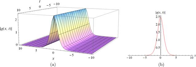
Figure 4. (a) 3D profile of the solution (36) with a = −0.1, b2 = −0.5, α4 = 0.1, b1 = 1, α2 = 1, k = ω = 1 (b) 2D curve for t = 1.
Type 4. If ${c}_{0}=\tfrac{{c}_{4}^{3}{m}^{2}}{32{c}_{6}^{2}\left({m}^{2}-1\right)},\,{c}_{2}=\tfrac{{c}_{4}^{2}\left(5{m}^{2}-4\right)}{16{c}_{6}\left({m}^{2}-1\right)},\,{c}_{6}\lt 0,$ then the equation (1) has the JEFs solutions:
$\begin{eqnarray}\begin{array}{l}q(x,t)=\displaystyle \frac{1}{12}\left[-\displaystyle \frac{5{b}_{1}}{{b}_{2}}+\displaystyle \frac{{\alpha }_{2}^{2}}{\left(1-{m}^{2}\right){\alpha }_{4}}\left(\Space{0ex}{3.20ex}{0ex}-2+{m}^{2}\right.\right.\\ \left.\left.+3{\mathrm{dn}}^{2}\left(-\displaystyle \frac{{\alpha }_{2}}{4}\sqrt{\displaystyle \frac{{b}_{2}}{5a\left(1-{m}^{2}\right){\alpha }_{4}}}\,\zeta \right)\right)\right]{{\rm{e}}}^{{\rm{i}}(\psi (\zeta )+\omega t)},\end{array}\end{eqnarray}$
or
$\begin{eqnarray}\begin{array}{l}q(x,t)=\displaystyle \frac{1}{12}\left[-\displaystyle \frac{5{b}_{1}}{{b}_{2}}+\displaystyle \frac{{\alpha }_{2}^{2}}{\left(1-{m}^{2}\right){\alpha }_{4}}\left(\Space{0ex}{5.25ex}{0ex}-2+{m}^{2}\right.\right.\\ \left.\left.+\displaystyle \frac{3\left(1-{m}^{2}\right)}{{\mathrm{dn}}^{2}\left(-\tfrac{{\alpha }_{2}}{4}\sqrt{\tfrac{{b}_{2}}{5a\left(1-{m}^{2}\right){\alpha }_{4}}}\,\zeta \right)}\right)\right]{{\rm{e}}}^{{\rm{i}}(\psi (\zeta )+\omega t)},\end{array}\end{eqnarray}$
with ab2α4 > 0. If m tends to 0, then $\mathrm{dn}(\zeta )$ tends to 1, and from solutions (37) and (38) become constants.
Type 5. If ${c}_{0}=\tfrac{{c}_{4}^{3}}{32{c}_{6}^{2}\left(1-{m}^{2}\right)},\,{c}_{2}=\tfrac{{c}_{4}^{2}\left(4{m}^{2}-5\right)}{16{c}_{6}\left({m}^{2}-1\right)},\,{c}_{6}\gt 0,$ then the JEFs solutions of equation (1) as:
$\begin{eqnarray}\begin{array}{l}q(x,t)=\displaystyle \frac{1}{12}\left[-\displaystyle \frac{5{b}_{1}}{{b}_{2}}+\displaystyle \frac{{\alpha }_{2}^{2}}{{\alpha }_{4}}\left(\displaystyle \frac{\left(1-2{m}^{2}\right)}{\left(-1+{m}^{2}\right)}\right.\right.\\ \left.\left.+\displaystyle \frac{3}{{\mathrm{cn}}^{2}\left(-\tfrac{{\alpha }_{2}}{4}\sqrt{-\tfrac{{b}_{2}}{5a\left(1-{m}^{2}\right){\alpha }_{4}}}\,\zeta \right)}\right)\right]{{\rm{e}}}^{{\rm{i}}(\psi (\zeta )+\omega t)},\end{array}\end{eqnarray}$
or
$\begin{eqnarray}\begin{array}{l}q(x,t)=\displaystyle \frac{1}{12}\left[-\displaystyle \frac{5{b}_{1}}{{b}_{2}}+\displaystyle \frac{{\alpha }_{2}^{2}}{{\alpha }_{4}}\left(\displaystyle \frac{\left(1-2{m}^{2}\right)}{\left(-1+{m}^{2}\right)}\right.\right.\\ \left.\left.+\displaystyle \frac{3{\mathrm{dn}}^{2}\left(-\tfrac{{\alpha }_{2}}{4}\sqrt{-\tfrac{{b}_{2}}{5a\left(1-{m}^{2}\right){\alpha }_{4}}}\,\zeta \right)}{\left(1-{m}^{2}\right){\mathrm{sn}}^{2}\left(-\tfrac{{\alpha }_{2}}{4}\sqrt{-\tfrac{{b}_{2}}{5a\left(1-{m}^{2}\right){\alpha }_{4}}}\,\zeta \right)}\right)\right]{{\rm{e}}}^{{\rm{i}}(\psi (\zeta )+\omega t)},\end{array}\end{eqnarray}$
with ab2α4 < 0. If m tends to 0, then $\mathrm{dn}(\zeta )$ tends to 1, $\mathrm{cn}(\zeta )$ tends to $\cos (\zeta )$, $\mathrm{sn}(\zeta )$ tends to $\sin (\zeta )$ and so from solution (40), we acquire the singular periodic wave solution (33). From (39), we obtain the periodic wave solution
$\begin{eqnarray}\begin{array}{l}q(x,t)=\displaystyle \frac{1}{12}\left[-\displaystyle \frac{5{b}_{1}}{{b}_{2}}+\displaystyle \frac{{\alpha }_{2}^{2}}{{\alpha }_{4}}\left(\Space{0ex}{3.05ex}{0ex}-1\right.\right.\\ \left.\left.+3\,{\sec }^{2}\left(-\displaystyle \frac{{\alpha }_{2}}{4}\sqrt{-\displaystyle \frac{{b}_{2}}{5a{\alpha }_{4}}}\,\zeta \right)\right)\right]{{\rm{e}}}^{{\rm{i}}(\psi (\zeta )+\omega t)}.\end{array}\end{eqnarray}$
The dynamical behaviors of solution (41) is presented in figure 5.
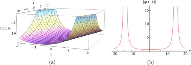
Figure 5. (a) 3D profile of the solution (41) with m = a = b1 = b2 = α2 = 1, α4 = −1, k = ω = 1 (b) 2D curve for t = 1.
Type 6. If ${c}_{0}=\tfrac{{c}_{4}^{3}{m}^{2}}{32{c}_{6}^{2}},\,{c}_{2}=\tfrac{{c}_{4}^{2}\left({m}^{2}+4\right)}{16{c}_{6}},\,{c}_{6}\lt 0,$ then the JEFs solutions of equation (1) as:
$\begin{eqnarray}\begin{array}{l}q(x,t)=\displaystyle \frac{1}{12}\left[-\displaystyle \frac{5{b}_{1}}{{b}_{2}}+\displaystyle \frac{{\alpha }_{2}^{2}}{{\alpha }_{4}}\left(-2+{m}^{2}\right.\right.\\ \left.\left.+3{\mathrm{dn}}^{2}\left(\displaystyle \frac{{\alpha }_{2}}{4}\sqrt{\displaystyle \frac{{b}_{2}}{5a{\alpha }_{4}}}\,\zeta \right)\right)\right]{{\rm{e}}}^{{\rm{i}}(\psi (\zeta )+\omega t)},\end{array}\end{eqnarray}$
or
$\begin{eqnarray}\begin{array}{l}q(x,t)=\displaystyle \frac{1}{12}\left[-\displaystyle \frac{5{b}_{1}}{{b}_{2}}+\displaystyle \frac{{\alpha }_{2}^{2}}{{\alpha }_{4}}\left(\Space{0ex}{4.75ex}{0ex}-2+{m}^{2}\right.\right.\\ \left.\left.-\displaystyle \frac{3\left(-1+{m}^{2}\right)}{{\mathrm{dn}}^{2}\left(\tfrac{{\alpha }_{2}}{4}\sqrt{\tfrac{{b}_{2}}{5a{\alpha }_{4}}}\,\zeta \right)}\right)\right]{{\rm{e}}}^{{\rm{i}}(\psi (\zeta )+\omega t)},\end{array}\end{eqnarray}$
with ab2α4 > 0. If m tends to 1, then $\mathrm{dn}(\zeta )$ tends to ${\rm{sech}} $, and on account of this from solution (42), we recover bright solitary wave solution (36).

5. Linear stability analysis

According to the linear stability analysis [32, 33], the constant solutions of equation (1) of the form:
$\begin{eqnarray}q={q}_{0}\,{{\rm{e}}}^{{\rm{i}}({kx}+\omega t)},\end{eqnarray}$
where q0 is the real constant-amplitudes (initial incidence power) while k and ω are the wave number and perturbation frequency. Substituting equation (44) into equation (1), we get
$\begin{eqnarray}\omega ={b}_{2}{q}_{0}^{2}-{{ak}}^{2}{q}_{0}+{b}_{1}{q}_{0}.\end{eqnarray}$
Assume that the perturbed solution of equation (1) of the form:
$\begin{eqnarray}q=\left[{q}_{0}+\theta \tilde{q}(x,t)\right]\,{{\rm{e}}}^{{\rm{i}}({kx}+\omega t)},\end{eqnarray}$
where θ << 1 is a perturbation parameter and $\tilde{q}$ can be expressed as
$\begin{eqnarray}\tilde{q}(x,t)={q}_{1}\,{{\rm{e}}}^{{\rm{i}}\left(\hat{k}x-\hat{\omega }t\right)}+{q}_{2}{{\rm{e}}}^{-{\rm{i}}\left(\hat{k}x-\hat{\omega }t\right)},\end{eqnarray}$
where q1 and q2 are the constant while $\hat{k}$ and $\hat{\omega }$ are the wave number and perturbation frequency. Inserting equation (46) into equation (1), we obtain
$\begin{eqnarray}2m\tilde{q}(x,t)+2i{\tilde{q}}_{t}+6{\rm{i}}{{akq}}_{0}{\tilde{q}}_{x}+3{{aq}}_{0}{\tilde{q}}_{{xx}}+2m\tilde{\mathrm{qc}}+2{\rm{i}}{{akq}}_{0}{\tilde{\mathrm{qc}}}_{x}+{{aq}}_{0}{\tilde{\mathrm{qc}}}_{{xx}}=0,\end{eqnarray}$
here $m=\tfrac{1}{2}{q}_{0}\left(-{{ak}}^{2}+{b}_{1}+2{b}_{2}{q}_{0}\right)$. Substituting equation (47) into equation (48) and linearizing equations about q1 and q2, we get:
$\begin{eqnarray*}{\psi }_{11}{q}_{1}+{\psi }_{12}{q}_{2}=0,\end{eqnarray*}$
$\begin{eqnarray}{\psi }_{21}{q}_{1}+{\psi }_{22}{q}_{2}=0,\end{eqnarray}$
where
$\begin{eqnarray*}\begin{array}{l}{\psi }_{11}=2m+a\hat{k}\left(2k-\hat{k}\right){q}_{0},\\ {\psi }_{12}=2\left(m-\hat{\omega }\right)+3a\hat{k}\left(2k-\hat{k}\right){q}_{0},\\ {\psi }_{21}=2\left(m+\hat{\omega }\right)-3a\hat{k}\left(2k+\hat{k}\right){q}_{0},\\ {\psi }_{22}=2m-a\hat{k}\left(2k+\hat{k}\right){q}_{0}.\end{array}\end{eqnarray*}$
Equation (49) has nonzero solutions if and only if
$\begin{eqnarray}\left|\begin{array}{ll}{\psi }_{11} & {\psi }_{12}\\ {\psi }_{21} & {\psi }_{22}\end{array}\right|=0.\end{eqnarray}$
Solving the above determinant, the following dispersion relation can be obtained:
$\begin{eqnarray}\hat{\omega }=3{ak}\hat{k}{q}_{0}\pm \sqrt{{\rm{\Delta }}},\end{eqnarray}$
where ${\rm{\Delta }}=a{\hat{k}}^{2}{q}_{0}\left[-2m+a\left({k}^{2}+2{\hat{k}}^{2}\right){q}_{0}\right]$.
If Δ ≥ 0, then $\hat{\omega }$ is real and hence the state for equation (1) is stable. Contrarily, if Δ < 0, then $\hat{\omega }$ is imaginary and the state for equation (1) becomes unstable. The growth rate of modulation instability gain spectrum G(k) can be derived as follows:
$\begin{eqnarray}G(k)=2\mathrm{Im}(\hat{\omega })=2\mathrm{Im}\left[3{ak}\hat{k}{q}_{0}\pm \sqrt{{\rm{\Delta }}}\right].\end{eqnarray}$
From figure 6, one can see that the MI growth rate increases with the increase of the incidence power q0.
Figure 6. G(k) for equation (1) when a = b1 = b2 = 0.1, k = 0.2 and q0 = 1, 2, 3 (from bottom to up).

6. Graphical interpretations

In this section, we present, the chirped soliton solutions of equation (1) are described graphically. Some of the obtained solutions are depicted by selecting different values of parameters to understand the physical meaning. In each figure, we display the 3D plot of the modulus and the 2D plot of their corresponding chirp. For example, the plots of the modulus of chirped dark soliton solution (29) and the chirped singular soliton solution (30) are represented with different values of parameters in figures 1 and 2 respectively. Figure 3 demonstrates the plot of the modulus of chirped singular periodic wave solution (33). The modulus of chirped bright soliton solution (36) is depicted in figure 4 while the modulus of the periodic wave solution (41) is presented in figure 5. On the other hand, figure 6, shows the MI gain spectra in normal dispersion regime.

7. Conclusions

In this paper, we have considered a nonlinear Schrödinger equation with nonlinear chromatic dispersion and quadratic-cubic law of refractive index. The NEAE method is utilized to obtain chirped optical soliton solutions of the considered model. Consequently, various types of chirped soliton solutions including dark, bright, singular and periodic soliton solutions are extracted from the JEF solutions when the modulus m → 1 or m → 0. The stability of the suggested model is shown by practicing the modulation instability analysis which verifies that the model is stable and confirms that all the obtained solutions are explicit, exact, reliable and stable. It is very clear that our promoted technique is effective, reliable, powerful, and friendly applicable and delivers sufficient well-matched explanations to NLPDEs arise in engineering, applied mathematics, nonlinear dynamics and mathematical physics. Further, the obtained results are illustrated in the form of a 3D plot and 2D curve by choosing proper parametric values to interpret the dynamics of wave profiles. So, by allotting appropriate quantities to the parameters, uncommon types of chirped soliton solutions are shown graphically. In future work, we aim to recover chirped optical soliton solutions for different forms of the nonlinear refractive index of an optical fiber when the corresponding CD is rendered to be nonlinear.
1
Iqbal M A Wang Y Miah M M Osman M S 2022 Study on Date–Jimbo–Kashiwara–Miwa equation with conformable derivative dependent on time parameter to find the exact dynamic wave solutions Fractal Fract. 6 4

DOI

2
Chu Y-M Nazir U Sohail M Selim M M Lee J-R 2021 Enhancement in thermal energy and solute particles using hybrid nanoparticles by engaging activation energy and chemical reaction over a parabolic surface via finite element approach Fractal Fract. 5 119

DOI

3
He Z-Y Abbes A Jahanshahi H Alotaibi N D Wang Y 2022 Fractional-order discrete-time SIR epidemic model with vaccination: Chaos and complexity Mathematics 10 165

DOI

4
Hashemi M S Darvishi E Baleanu D 2016 A geometric approach for solving the density-dependent diffusion Nagumo equation Adv. Diff. Equ. 2016 1 13

DOI

5
Mathanaranjan T 2022 New optical solitons and modulation instability analysis of generalized coupled nonlinear Schrödinger–KdV system Opt. Quantum Electron. 54 336

DOI

6
Park C Nuruddeen R I Ali K K Muhammad L Osman M S Baleanu D 2020 Novel hyperbolic and exponential ansatz methods to the fractional fifth-order Korteweg–de Vries equations Adv. Diff. Equ. 2020 1 12

DOI

7
Arnous A H Mirzazadeh M 2016 Application of the generalized Kudryashov method to the Eckhaus equation Nonlinear Anal.: Model Control 21 577 586

DOI

8
Yusuf A Sulaiman T A Inc M Bayram M 2020 Breather wave, lump-periodic solutions and some other interaction phenomena to the Caudrey–Dodd–Gibbon equation Eur. Phys. J. Plus 135 1 8

DOI

9
Lei Z-Q Liu J-G Rezazadeh H Khater M M A Inc M 2021 Research of lump dynamics on the (3+1)-dimensional B-type Kadomtsev–Petviashvili–Boussinesq equation Mod. Phys. Lett. B 35 2150474

DOI

10
Matveen V B Salle M A 1991 Darboux Transformations and Solitons Berlin Springer

11
Wang X-B Tian S-F 2022 Exotic vector freak waves in the nonlocal nonlinear Schrödinger equation Physica D 442 133528

DOI

12
Zhou Q Ekici M Sonmezoglu A Mirzazadeh M Eslami M 2016 Optical solitons with Biswas–Milovic equation by extended trial equation method Nonlinear Dyn. 84 1883 1900

DOI

13
Akbulut A Mirzazadeh M Hashemi M S Hosseini K Salahshour S Park C 2023 Triki–Biswas model: its symmetry reduction, Nucci's reduction and conservation laws Int. J. Mod. Phys. B 37 2350063

DOI

14
Hosseini K Akbulut A Baleanu D Salahshour S 2022 The Sharma–Tasso–Olver–Burgers equation: its conservation laws and kink solitons Commun. Theor. Phys. 74 025001

DOI

15
Mirzazadeh M Akbulut A Taşcan F Akinyemi L 2022 A novel integration approach to study the perturbed Biswas-Milovic equation with Kudryashov's law of refractive index Optik 252 168529

DOI

16
Hashemi M S 2018 Some new exact solutions of (2+1)-dimensional nonlinear Heisenberg ferromagnetic spin chain with the conformable time fractional derivative Opt. Quantum Electron. 50 1 11

DOI

17
Hashemi M S 2021 A novel approach to find exact solutions of fractional evolution equations with non-singular kernel derivative Chaos, Solitons Fractals 152 111367

DOI

18
Mathanaranjan T 2023 Optical solitons and stability analysis for the new (3+1)-dimensional nonlinear Schrödinger equation J. Nonlinear Opt. Phys. Mater. 32 2350016

DOI

19
Zayed E M E Alurrfi K A E 2016 New extended auxiliary equation method and its applications to nonlinear Schrödinger-type equations Optik 127 9131 9151

DOI

20
Zayed E M Alngar M E El-Horbaty M Biswas A Yıldırım Y Alshomrani A S Belic M R 2020 Chirped and chirp-free optical solitons having generalized anti-cubic nonlinearity with a few cutting-edge integration technologies Optik 206 163745

DOI

21
Mia R Miah M M Osman M S 2023 A new implementation of a novel analytical method for finding the analytical solutions of the (2+1)-dimensional KP-BBM equation Heliyon 9 e15690

DOI

22
Siddique I Jaradat M M Zafar A Mehdi K B Osman M S 2021 Exact traveling wave solutions for two prolific conformable M-Fractional differential equations via three diverse approaches Results Phys. 28 104557

DOI

23
Ashik Iqbal M Baleanu D Mamun Miah M Shahadat Ali H M Hashim Alshehri M Osman M S 2023 New soliton solutions of the mZK equation and the Gerdjikov-Ivanov equation by employing the double $G^{\prime} /G,1/G$-expansion method Results Phys. 47 106391

DOI

24
Nisar K S Ilhan O A Abdulazeez S T Manafian J Mohammed S A Osman M S 2021 Novel multiple soliton solutions for some nonlinear PDEs via multiple Exp-function method Results Phys. 21 103769

DOI

25
Mathanaranjan T 2022 An effective technique for the conformable space-time fractional cubic-quartic nonlinear Schrodinger equation with different laws of nonlinearity Comput. Methods Diff. Equ. 10 701 715

DOI

26
Az-Zobi E Al-Maaitah A F Tashtoush M A Osman M S 2022 New generalised cubic-quintic-septic NLSE and its optical solitons Pramana 96 184

DOI

27
Mathanaranjan T 2020 Solitary wave solutions of the Camassa–Holm nonlinear Schrödinger equation Results Phys. 19 103549

DOI

28
Chu Y Rashid S Kubra K T Inc M Hammouch Z Osman M S 2023 CMES-Comput. Model. Eng. Sci. 136 3025 3060

DOI

29
Mathanaranjan T Himalini K 2019 Analytical solutions of the time-fractional non-linear Schrödinger equation with zero and non zero trapping potential through the Sumudu Decomposition method J. Sci. Univ. Kelaniya 12 21 33

DOI

30
Adem A R Ekici M Biswas A Asma M Zayed E M Alzahrani A K Belic M R 2020 Stationary optical solitons with nonlinear chromatic dispersion having quadratic-cubic law of refractive index Phys. Lett. A 384 126606

DOI

31
Bouzida A Triki H Ullah M Z Zhou Q Biswas A Belic M 2017 Chirped optical solitons in nano optical fibers with dual-power law nonlinearity Optik 142 77 81

DOI

32
Agrawal G P 2013 Nonlinear fiber optics Cambridge, MA Academic Press 44

DOI

33
Liu W Zhang Y 2019 Optical soliton solutions, explicit power series solutions and linear stability analysis of the quintic derivative nonlinear Schrödinger equation Opt. Quantum Electron. 51 1 13

DOI

Outlines

/