


1. Introduction
Symmetry study has been widely studied in nonlinear science. The Lie group method plays an important role in seeking solutions of nonlinear partial differential equations (NLPEs) [1, 2]. The special solutions of a given equation can be obtained in terms of solutions of lower dimensional equations [3]. Compared with Lie point symmetry, many nonlocal symmetries and corresponding group invariant solutions are obtained by the Painlevé analysis and Lax pair [4–7]. Lie point symmetries and the related Kac–Moody–Virasoro algebra of the Kadomtsev–Petviashvili equation have been constructed by using the standard classical Lie approach [8]. The generalized symmetries and the generalized W∞ symmetry algebra are derived through the formal series symmetry approach [9–11]. The generalized W∞ symmetry algebra will reduce to the Virasoro algebra with certain parameters [10]. An isomorphic centerless Virasoro symmetry algebra is found in the (2+1)-dimensional and the (3+1)-dimensional integrable models [12–16]. The formal series symmetry approach [9, 10] and the master symmetry approach [17, 18] can be successfully applied to find infinitely many generalized symmetries. The related topics of symmetry have triggered interest in (2+1)-dimensional soliton systems. Naturally, an important problem is whether other (2+1)-dimensional systems possess the Kac–Moody–Virasoro algebra and the centerless Virasoro symmetry algebra.
Recently, a (2+1)-dimensional Korteweg–de Vries–Sawada–Kotera–Ramani (KdVSKR) equation is proposed to describe the resonances of solitons in shallow water [19, 20]. The (2+1)-dimensional KdVSKR equation reads as [19]1 ) reduces to the standard KdV equation and the (2+1)-dimensional SK equation with β = 0 and α = 0, respectively. The KdVSKR equation (1 ) possesses a rich physical meaning in nonlinear science. The standard KdV equation and the (2+1)-dimensional SK equation are completely integrable by means of the inverse scattering transform method [21]. Soliton molecules and full symmetry groups of the (1+1)-dimensional KdVSKR equation are obtained by the Hirota bilinear and the symmetry group direct methods [22]. The soliton molecules, the multi-breathers, and the interactions between the soliton molecule and breathers/lumps of (1 ) are explored by the velocity mechanism [20].
$\begin{eqnarray}\begin{array}{l}{u}_{t}+\alpha ({u}_{{xxx}}+6{{uu}}_{x})-\beta ({u}_{{xxxxx}}+45{u}^{2}{u}_{x}\\ \quad +15{{uu}}_{y}+15{{uu}}_{{xxx}}+15{u}_{x}{u}_{{xx}}\end{array}\end{eqnarray}$
$\begin{eqnarray*}+5{u}_{{xxy}}-5{w}_{y}+15{u}_{x}w)=0,\end{eqnarray*}$
$\begin{eqnarray}{u}_{y}={w}_{x},\end{eqnarray}$
where α and β are arbitrary constants. The (2+1)-dimensional KdVSKR equation (The purpose of this work is to study the integrable property and the symmetry group of the KdVSKR equation. The outline of the paper is arranged as follows. In section 2 , the Painlevé property of the (2+1)-dimensional KdVSKR equation is studied by the standard singularity analysis. In section 3 , the symmetry algebra and the infinite-dimensional symmetry group of the model are established by the Lie point symmetry. In section 4 , some physical meanings of the finite-dimensional algebras are obtained by restricting the arbitrary functions of t to first degree polynomials. By selecting the Laurent polynomials in t, the commutation relations of the subalgebra are calculated. In section 5 , the group invariant solutions are obtained by the corresponding symmetry reductions. The conclusions are discussed in section 6 .
2. Painlevé analysis of the KdVSKR equation
The integrability of the NLPEs is studied by various methods. Among these methods, the standard Painlevé method, i.e. the Weiss–Tabor–Carnevale (WTC) method [23], is widely used to verify the integrable conditions of given NLPEs [23–25]. In this section, we shall study the integrability of the (2+1)-dimensional KdVSKR equation (1 ) with the WTC method.
According to the WTC approach, the Painlevé test includes three steps: the leading order analysis, resonant point determination and resonance condition verification. While all the movable singularities of their solutions are only poles, the model is called the Painlevé integrable system. The fields u and w are expanded about the singularity manifold φ(x, y, t) = 0 as5 ) into (1 ), the coefficients of (φj−7, φj−3) are1 ) passes the Painlevé test in the sense of the WTC method.
$\begin{eqnarray}u=\displaystyle \sum _{j=0}^{\infty }{u}_{j}{\phi }^{j-{\alpha }_{1}},\qquad w=\displaystyle \sum _{j=0}^{\infty }{w}_{j}{\phi }^{j-{\alpha }_{2}},\end{eqnarray}$
where uj and wj are the arbitrary functions of x, y, t. By the leading order analysis, the constants α1 and α2 are positive integers. The values of α1 and α2 read $\begin{eqnarray}{\alpha }_{1}=2,\qquad {\alpha }_{2}=2,\end{eqnarray}$
and the functions u0 and w0 are $\begin{eqnarray}{u}_{0}=-2{\phi }_{x}^{2},\qquad {w}_{0}=2{\phi }_{x}{\phi }_{y}.\end{eqnarray}$
The Laurent expansion of the solution in the neighbourhood of the singular manifold becomes $\begin{eqnarray}\begin{array}{rcl}u & = & \displaystyle \frac{-2{\phi }_{x}^{2}}{{\phi }^{2}}+\displaystyle \frac{{u}_{1}}{\phi }+\displaystyle \sum _{j=1}^{\infty }{u}_{j}{\phi }^{j-1},\\ w & = & \displaystyle \frac{-2{\phi }_{x}{\phi }_{y}}{{\phi }^{2}}+\displaystyle \frac{{w}_{1}}{\phi }+\displaystyle \sum _{j=2}^{\infty }{w}_{j}{\phi }^{j-2}.\end{array}\end{eqnarray}$
By substituting ( $\begin{eqnarray}\begin{array}{l}\left(\begin{array}{cc}(j+1)(j-2)(j-3)(j-6)(j-10)\beta {\phi }_{x}^{5} & 0\\ -(j-2){\phi }_{y} & (j-2){\phi }_{x}\end{array}\right)\\ \quad \times \,\left(\begin{array}{c}{u}_{j}\\ {w}_{j}\end{array}\right)\,=\,0.\end{array}\end{eqnarray}$
The values of the resonances are $\begin{eqnarray}j=-1,2,2,3,6,10.\end{eqnarray}$
The resonance at j = −1 represents the arbitrariness of the singularity manifold φ(x, y, t) = 0. The functions of u1 and w1 read as u1 = 2φxx, w1 = 2φxy by selecting the coefficients of (φ−6, φ−2). To verify the existence of arbitrary functions at other resonance values, we proceed with the coefficients of (φ−5, φ−1). The resonances at j = 2, 2 represent the arbitrary functions u1 and w1. By collecting the coefficients of (φ−4, φ0), the functions of u2 and w2 satisfy the relation w3φx − u3φy + w2x + u2y = 0. Either of the functions u3 and w3 is thus an arbitrary function. The functions w4 and w6 are arbitrary at the resonances j = 6 and j = 10, respectively. From the above analysis, the number of arbitrary functions is the same as the number of resonances and (3. Lie point symmetry of the KdVSKR equation
Based on the Lie point symmetry method [1], the KdVSKR equation is invariance under transformation1 )11 ) into the symmetry equations (10 ) and taking u and w to satisfy the KdVSKR system. Solving the over-determined equations leads to the infinitesimals
$\begin{eqnarray}u\to u+\epsilon {\sigma }^{u},\qquad w\to w+\epsilon {\sigma }^{w},\end{eqnarray}$
where ε is the infinitesimal parameter. The general vector field reads $\begin{eqnarray}V=T\displaystyle \frac{\partial }{\partial t}+X\displaystyle \frac{\partial }{\partial x}+Y\displaystyle \frac{\partial }{\partial y}+U\displaystyle \frac{\partial }{\partial u}+W\displaystyle \frac{\partial }{\partial w},\end{eqnarray}$
where T, X, Y, U and W are the functions of t, x, y, u and w. The symmetry equations for σu and σw are expressed as a solution of the linearized system ( $\begin{eqnarray}\begin{array}{l}{\sigma }_{\,t}^{u}-\alpha [6{\left({\sigma }^{u}u\right)}_{x}+{\sigma }_{{xxx}}^{u}]-\beta [45{\left({u}^{2}{\sigma }^{u}\right)}_{x}\\ \quad +15{\left(u{\sigma }_{{xx}}^{u}\right)}_{x}+15{\left({\sigma }^{u}w\right)}_{x}+15{\left({\sigma }^{u}u\right)}_{y}\end{array}\end{eqnarray}$
$\begin{eqnarray*}+15{\left({\sigma }^{u}{u}_{{xx}}\right)}_{x}-5{\sigma }_{\,y}^{w}+{\sigma }_{{xxy}}^{u}+{\sigma }_{{xxxxx}}^{u}]=0,\end{eqnarray*}$
$\begin{eqnarray}{\sigma }_{\,y}^{u}={\sigma }_{\,x}^{w}.\end{eqnarray}$
The corresponding symmetries of σu and σw are $\begin{eqnarray}\begin{array}{rcl}{\sigma }^{u} & = & {{Tu}}_{t}+{{Xu}}_{x}+{{Yu}}_{y}-U,\\ {\sigma }^{w} & = & {{Tw}}_{t}+{{Xw}}_{x}+{{Yw}}_{y}-W.\end{array}\end{eqnarray}$
Over-determined equations of the KdVSKR system can be obtained by substituting ( $\begin{eqnarray}\begin{array}{rcl}T & = & f(t),\qquad X=\displaystyle \frac{1}{5}\dot{f}(t)x-\displaystyle \frac{2\alpha }{75\beta }\dot{f}(t)y\\ & & -\displaystyle \frac{1}{50\beta }\ddot{f}(t){y}^{2}-\displaystyle \frac{1}{15\beta }\dot{g}(t)y+h(t),\\ Y & = & \displaystyle \frac{3}{5}\dot{f}(t)y+g(t),\qquad U=-\displaystyle \frac{2}{5}\dot{f}(t)u\\ & & +\displaystyle \frac{4\alpha }{225\beta }\dot{f}(t)-\displaystyle \frac{1}{75\beta }\ddot{f}(t)y-\displaystyle \frac{1}{45\beta }\dot{g}(t),\\ W & = & -\displaystyle \frac{4}{5}\dot{f}(t)w+\displaystyle \frac{1}{25\beta }\ddot{f}(t){yu}+\displaystyle \frac{2\alpha }{75\beta }\dot{f}(t)u\\ & & -\displaystyle \frac{4\alpha }{1125{\beta }^{2}}\ddot{f}(t)y-\displaystyle \frac{1}{75\beta }\ddot{f}(t)x+\displaystyle \frac{1}{15\beta }\dot{g}(t)u\\ & & +\displaystyle \frac{8{\alpha }^{2}}{1125{\beta }^{2}}\dot{f}(t)+\displaystyle \frac{1}{750{\beta }^{2}}\dddot{f}(t){y}^{2}-\displaystyle \frac{2\alpha }{225{\beta }^{2}}\dot{g}(t)\\ & & +\displaystyle \frac{1}{225{\beta }^{2}}\ddot{g}(t)y-\displaystyle \frac{1}{15\beta }\dot{h}(t),\end{array}\end{eqnarray}$
where f(t), g(t) and h(t) are the arbitrary functions of t and the dots indicate derivatives with respect to t. The corresponding vector is $\begin{eqnarray}V=P(f)+Q(g)+R(h),\end{eqnarray}$
with P(f), Q(g) and R(h) $\begin{eqnarray}\begin{array}{l}P(f)=f(t)\displaystyle \frac{\partial }{\partial t}+\left[\displaystyle \frac{1}{5}\dot{f}(t)x-\displaystyle \frac{2\alpha }{75\beta }\dot{f}(t)y-\displaystyle \frac{1}{50\beta }\ddot{f}(t){y}^{2}\right]\\ \,\times \displaystyle \frac{\partial }{\partial x}+\displaystyle \frac{3}{5}\dot{f}(t)y\displaystyle \frac{\partial }{\partial y}+\left[-\displaystyle \frac{2}{5}u\dot{f}(t)+\displaystyle \frac{4\alpha }{225\beta }\dot{f}(t)-\displaystyle \frac{1}{75\beta }\ddot{f}(t)y\right]\\ \quad \times \displaystyle \frac{\partial }{\partial u}+\left[-\displaystyle \frac{4}{5}\dot{f}(t)w+\displaystyle \frac{1}{25\beta }\ddot{f}(t){uy}+\displaystyle \frac{2\alpha }{75\beta }\dot{f}(t)u\right.\end{array}\end{eqnarray}$
$\begin{eqnarray}\begin{array}{l}\quad +\displaystyle \frac{8{\alpha }^{2}}{1125{\beta }^{2}}\dot{f}(t)-\displaystyle \frac{4\alpha }{1125{\beta }^{2}}\ddot{f}(t)y-\displaystyle \frac{1}{75\beta }\ddot{f}(t)x\\ \quad \left.+\displaystyle \frac{1}{750{\beta }^{2}}\dddot{f}(t){y}^{2}\right]\displaystyle \frac{\partial }{\partial w},\\ Q(g)=-\displaystyle \frac{1}{15\beta }\dot{g}(t)\displaystyle \frac{\partial }{\partial x}+g(t)\displaystyle \frac{\partial }{\partial y}-\displaystyle \frac{1}{45\beta }\dot{g}(t)\displaystyle \frac{\partial }{\partial u}\\ \quad +\left[\displaystyle \frac{1}{15\beta }\dot{g}(t)u-\displaystyle \frac{2\alpha }{225{\beta }^{2}}\dot{g}(t)+\displaystyle \frac{1}{225{\beta }^{2}}\ddot{g}(t)y\right]\displaystyle \frac{\partial }{\partial w},\\ R(h)=h(t)\displaystyle \frac{\partial }{\partial x}-\displaystyle \frac{1}{15\beta }\dot{h}(t)\displaystyle \frac{\partial }{\partial w}.\end{array}\end{eqnarray}$
4. Symmetry group of KdVSKR equation
The commutation relations of the infinite-dimensional Lie algebra (14 ) are15 ). The KdVSKR system possesses the Virasoro symmetry structure.
$\begin{eqnarray}\left[P({f}_{1}),P({f}_{2})\right]=P({f}_{1}\dot{{f}_{2}}-{f}_{2}\dot{{f}_{1}}),\end{eqnarray}$
$\begin{eqnarray}\left[P(f),Q(g)\right]=Q(f\dot{g}-\displaystyle \frac{3}{5}g\dot{f}),\end{eqnarray}$
$\begin{eqnarray}\left[P(f),R(h)\right]=R(f\dot{h}-\displaystyle \frac{1}{5}h\dot{f}),\end{eqnarray}$
$\begin{eqnarray}\left[Q({g}_{1}),Q({g}_{2})\right]=\displaystyle \frac{1}{15\beta }Q(\dot{{g}_{1}}{g}_{2}-{g}_{1}\dot{{g}_{2}}),\end{eqnarray}$
$\begin{eqnarray}\left[Q(g),R(h)\right]=[R({h}_{1}),R({h}_{2})]=0.\end{eqnarray}$
It is shown that each term of P(f), Q(g) and R(h) constitutes Kac–Moody–Virasoro type algebra. The subalgebra for P(f) is just the Virasoro symmetry algebra from (Some physical symmetries of the KdVSKR equation can be obtained by restricting the arbitrary functions f(t), g(t) and h(t) to be first-order polynomials in t. By restricting the arbitrary functions f(t), g(t) and h(t) to be first-order polynomials in t, a finite-dimensional subalgebra of physical transformations can be obtained
$\begin{eqnarray}\begin{array}{rcl}M & = & P(1)={\partial }_{t},\\ N & = & P(t)=t{\partial }_{t}+\left(\displaystyle \frac{x}{5}-\displaystyle \frac{2\alpha }{75\beta }y\right){\partial }_{x}+\displaystyle \frac{3}{5}y{\partial }_{y}\\ & & +\left(\displaystyle \frac{4\alpha }{225\beta }-\displaystyle \frac{2}{5}u\right){\partial }_{u}+\left(\displaystyle \frac{2\alpha }{75\beta }u\right.\left.-\displaystyle \frac{4}{5}w+\displaystyle \frac{8{\alpha }^{2}}{1125{\beta }^{2}}\right){\partial }_{w},\\ L & = & Q(1)={\partial }_{y},\qquad H=Q(t)=-\displaystyle \frac{1}{15\beta }y{\partial }_{x}\\ & & +t{\partial }_{y}-\displaystyle \frac{1}{45\beta }{\partial }_{u}+\left(\displaystyle \frac{1}{15\beta }u-\displaystyle \frac{2\alpha }{225{\beta }^{2}}\right){\partial }_{w},\\ K & = & R(1)={\partial }_{x},\qquad D=R(t)=t{\partial }_{x}-\displaystyle \frac{1}{15\beta }{\partial }_{w},\end{array}\end{eqnarray}$
where M, L and K are generated translations in the t, y and x, respectively, N is the generated dilations and a Galilei boost in the x direction, H has some properties of a rotation and a Galilei boost in the y direction, and D yields a Galilei transformation in the x direction.By using the functions f(t), g(t) and h(t) to be Laurent polynomials in t, the subalgebra reads
$\begin{eqnarray}\begin{array}{l}P({t}^{n})={t}^{n}\displaystyle \frac{\partial }{\partial t}+\displaystyle \frac{{{nt}}^{n}}{5}\left(\displaystyle \frac{x}{t}-\displaystyle \frac{2\alpha y}{15\beta t}-\displaystyle \frac{{{ny}}^{2}}{10\beta {t}^{2}}+\displaystyle \frac{{y}^{2}}{10\beta {t}^{2}}\right)\displaystyle \frac{\partial }{\partial x}\\ \quad +\displaystyle \frac{3}{5}{{nt}}^{n-1}y\displaystyle \frac{\partial }{\partial y}+\displaystyle \frac{{{nt}}^{n}}{5}\left(\displaystyle \frac{4\alpha }{45\beta t}-\displaystyle \frac{2u}{t}-\displaystyle \frac{{ny}}{15\beta {t}^{2}}\right.\\ \quad \left.+\displaystyle \frac{y}{15\beta {t}^{2}}\right)\displaystyle \frac{\partial }{\partial u}+\displaystyle \frac{{{nt}}^{n}}{1125{\beta }^{2}}\left[\displaystyle \frac{3{y}^{2}(n-1)(n-2)}{2{t}^{3}}+\displaystyle \frac{1}{{t}^{2}}(n-1)\right.\\ \quad \times (45y\beta u-4\alpha y-15\beta x)\\ \quad \left.+\displaystyle \frac{2}{t}(15\alpha \beta u-450{\beta }^{2}w+4{\alpha }^{2})\right]\displaystyle \frac{\partial }{\partial w},\\ Q({t}^{n})=-\displaystyle \frac{{{nt}}^{n-1}y}{15\beta }\displaystyle \frac{\partial }{\partial x}+{t}^{n}\displaystyle \frac{\partial }{\partial y}-\displaystyle \frac{{{nt}}^{n-1}}{45\beta }\displaystyle \frac{\partial }{\partial u}\\ \quad +\displaystyle \frac{{{nt}}^{n-2}}{225{\beta }^{2}}(15\beta {tu}-2\alpha t+{ny}-y)\displaystyle \frac{\partial }{\partial w},\\ R({t}^{n})={t}^{n}\displaystyle \frac{\partial }{\partial x}-\displaystyle \frac{{{nt}}^{n-1}}{15\beta }\displaystyle \frac{\partial }{\partial w},\end{array}\end{eqnarray}$
with n ∈ Z. The commutation relations of this subalgebra are $\begin{eqnarray}\begin{array}{rcl}\left[P({t}^{n}),P({t}^{m})\right] & = & (m-n)P({t}^{n+m-1}),\\ \left[P({t}^{n}),Q({t}^{m})\right] & = & \left(m-\displaystyle \frac{3}{5}n\right)Q({t}^{n+m-1}),\\ \left[P({t}^{n}),R({t}^{m})\right] & = & \left(m-\displaystyle \frac{1}{5}n\right)R({t}^{n+m-1}),\\ \left[Q({t}^{n}),Q({t}^{m})\right] & = & \displaystyle \frac{1}{15\beta }(m-n)Q({t}^{n+m-1}),\\ \left[Q({t}^{n}),R({t}^{m})\right] & = & [R({t}^{n}),R({t}^{m})]=0.\end{array}\end{eqnarray}$
The above symmetry constitutes a centerless Virasoro algebra which has been widely used in the field of physics [26].5. Similarity reductions of KdVSKR equation
The Lie symmetries, a one-dimensional optimal system and symmetry reductions of the nonlinear systems are presented in a systematic review [27–29]. The explicit solutions are obtained by solving the related characteristics equations. Based on the Lie group method, the group invariant solutions of the KdVSKR system can be obtained by solving the following characteristic equations
$\begin{eqnarray}\displaystyle \frac{{\rm{d}}t}{T}=\displaystyle \frac{{\rm{d}}x}{X}=\displaystyle \frac{{\rm{d}}y}{Y}=\displaystyle \frac{{\rm{d}}u}{U}=\displaystyle \frac{{\rm{d}}w}{W}.\end{eqnarray}$
For the similarity group solutions, three cases are listed.Case I. For the simplification form of the reduction system, we select f(t) = 1. The similarity solution is given by solving the characteristic equations25 ), the group invariant solution can be obtained by using (24 ).
$\begin{eqnarray}\begin{array}{rcl}u & = & U(\xi ,\eta )-\displaystyle \frac{g(t)}{45\beta },\\ w & = & \exp \left(\displaystyle \frac{-4t}{5}\right)W(\xi ,\eta )+\displaystyle \frac{2{\alpha }^{2}}{225{\beta }^{2}}+\displaystyle \frac{\exp \left(-\tfrac{4t}{5}\right)}{225\beta }\end{array}\end{eqnarray}$
$\begin{eqnarray}\begin{array}{rcl} & & \times {\int }_{0}^{t}\exp \left(\displaystyle \frac{4s}{5}\right)\left[\Space{0ex}{3ex}{0ex}15\dot{g}(s)U(\xi ,\eta )+6\alpha U(\xi ,\eta )\right.\\ & & -\displaystyle \frac{1}{3\beta }\dot{g}(s)g(s)-\displaystyle \frac{2\alpha }{\beta }\dot{g}(s)-\displaystyle \frac{2\alpha }{15\beta }g(s)\\ & & \left.-15\dot{h}(s)+\displaystyle \frac{\ddot{g}(s)}{\beta }\eta +\displaystyle \frac{\ddot{g}(s)}{\beta }{\int }_{0}^{s}g(m){dm}\right]{ds},\end{array}\end{eqnarray}$
with the similarity variables $\xi =\tfrac{g(t)y}{15\beta }-{\int }_{0}^{t}h(s){ds}+x$ and $\eta =y-{\int }_{0}^{t}g(s){ds}$. The group invariant functions U and W satisfy $\begin{eqnarray}\begin{array}{l}\left[\displaystyle \frac{g(t)}{15\beta }-\displaystyle \frac{\alpha }{30\beta }-\displaystyle \frac{\exp \left(-\tfrac{4t}{5}\right)}{15\beta }{\int }_{0}^{t}\exp \left(\displaystyle \frac{4s}{5}\right)\dot{g}(s){ds}\right]{U}_{\xi }\\ \quad -\exp \left(-\displaystyle \frac{4t}{5}\right){W}_{\xi }+{U}_{\eta }=0,\\ \quad \left[15\beta U+\displaystyle \frac{2}{3}g(t)\right]{U}_{\eta }+15\beta {U}_{\xi }{U}_{\xi \xi }-\exp \left(-\displaystyle \frac{4t}{5}\right)\\ \quad \times \left[5\beta {W}_{\eta }+\displaystyle \frac{g(t)}{3}{W}_{\xi }\right]+5\beta {U}_{\xi \xi \eta }+(15\beta U-\alpha ){U}_{\xi \xi \xi }\\ \quad +\beta {U}_{\xi \xi \xi \xi \xi }+\displaystyle \frac{g(t)}{45\beta }+15\exp \left(-\displaystyle \frac{4t}{5}\right)\beta {U}_{\xi }W+45\beta {U}_{\xi }{U}^{2}\\ \quad -[6\alpha +g(t)]{{UU}}_{\xi }-\displaystyle \frac{{U}_{\xi }}{15\beta }\left[\eta \dot{g}(t)-2{\alpha }^{2}\right.\\ \quad \left.+\dot{g}(t){\int }_{0}^{t}g(s){ds}-2\alpha g(t)-15\beta h(t)\right]-\displaystyle \frac{\exp \left(-\tfrac{4t}{5}\right)}{45}\\ \quad \times {\int }_{0}^{t}\exp \left(\displaystyle \frac{4s}{5}\right)\left[\dot{g}(s)g(t){U}_{\xi }+15\beta \dot{g}(s){U}_{\eta }\right.\\ \quad \left.+\displaystyle \frac{2\alpha }{15}g(s){U}_{\xi }+2\alpha \beta {U}_{\eta }+\ddot{g}(s)\right]{ds}+\exp \left(-\displaystyle \frac{4t}{5}\right){U}_{\xi }\\ \quad \times {\int }_{0}^{t}\exp \left(\displaystyle \frac{4s}{5}\right)\left[\dot{g}(s)U+\displaystyle \frac{2\alpha }{5}U-\displaystyle \frac{1}{45\beta }g(s)\dot{g}(s)\right.\\ \quad -\displaystyle \frac{2\alpha }{15\beta }\dot{g}(s)-\displaystyle \frac{2\alpha }{225\beta }g(s)+\displaystyle \frac{1}{15}\ddot{g}(s){\int }_{0}^{s}g(m){dm}\\ \quad \left.+\beta \dot{h}(s)+\displaystyle \frac{\eta }{15\beta }\ddot{g}(s)\right]{ds}=0.\end{array}\end{eqnarray}$
If we get the solution of (Case II. The similarity solution is derived by solving out the characteristic equations with f(t) = 026 ) into (1 ) satisfies the following equations
$\begin{eqnarray}\begin{array}{rcl}u & = & U(t,\eta )+\displaystyle \frac{{Mcsgn}(M)}{45\beta g(t)},\\ w & = & W(t,\eta )+\displaystyle \frac{{Mcsgn}(M)}{15\beta g(t)}U(t,\eta )+\displaystyle \frac{{Mcsgn}(M)}{15\beta g(t)}\\ & & \times \left(\displaystyle \frac{\ddot{g}(t)h(t)}{{\dot{g}}^{2}(t)}-\displaystyle \frac{\dot{h}(t)}{\dot{g}(t)}-\displaystyle \frac{2\alpha }{15\beta }\right)\\ & & +\displaystyle \frac{x}{15\beta }\left(\displaystyle \frac{\dot{g}(t)}{3g(t)}-\displaystyle \frac{\ddot{g}(t)}{\dot{g}(t)}\right),\end{array}\end{eqnarray}$
with $M=15\beta h(t)-y\dot{g}(t)$, the symbolic function csgn(M), the similarity variable $\eta =-\tfrac{\dot{g}(t)}{30\beta g(t)}{y}^{2}+\tfrac{h(t)}{g(t)}y-x$ and the group invariant functions U and W. Substituting ( $\begin{eqnarray}\begin{array}{l}{U}_{t}+\left[45\beta {U}^{2}-\left(6\alpha +\displaystyle \frac{M}{g(t)}+\displaystyle \frac{M}{g(t){csgn}(M)}\right)U\right.\\ \quad +15\beta W+\displaystyle \frac{2{M}^{2}({csgn}(M)+1)}{45\beta g{\left(t\right)}^{2}{csgn}(M)}+\displaystyle \frac{\eta (3\ddot{g}(t)g(t)-{\dot{g}}^{2}(t))}{3g(t)\dot{g}}\\ \quad \times \displaystyle \frac{M({csgn}(M)+1)(h(t)\ddot{g}(t)-\dot{g}(t)\dot{h}(t))}{{\dot{g}}^{2}(t)g(t){csgn}(M)}-\displaystyle \frac{15\beta {h}^{2}(t)\ddot{g}(t)}{g(t){\dot{g}}^{2}(t)}\\ \quad \left.-\displaystyle \frac{5\beta {h}^{2}(t)}{{g}^{2}(t)}+\displaystyle \frac{15\beta h(t)\dot{h}(t)}{g(t)\dot{g}(t)}\right]{U}_{\eta }+15\beta {U}_{\eta \eta }\\ \quad +\left(15\beta U-\alpha -\displaystyle \frac{M}{3g(t)}-\displaystyle \frac{M}{3g(t){csgn}(M)}\right){U}_{\eta \eta \eta }\\ \quad +\beta {U}_{\eta \eta \eta \eta \eta }+\displaystyle \frac{M}{3g(t)}{W}_{\eta }+\displaystyle \frac{\dot{g}(t)M}{135{g}^{2}(t)\beta }\\ \quad -\displaystyle \frac{2\dot{g}(t)U}{3g(t){csgn}(M)}+\displaystyle \frac{2\alpha \dot{g}}{45\beta g(t){csgn}(M)}\\ \quad -\displaystyle \frac{M\ddot{g}(t)}{45\beta \dot{g}(t)g(t){csgn}(M)}+\displaystyle \frac{\dot{g}(t)M}{45\beta g{\left(t\right)}^{2}{csgn}(M)}=0,\\ \quad {W}_{\eta }-\left[\displaystyle \frac{{csgn}(M)h(t)}{g(t)}+\displaystyle \frac{M}{15\beta g(t)}-\displaystyle \frac{y\dot{g}(t){csgn}(M)}{15\beta g(t)}\right]{U}_{\eta }\\ \quad -\displaystyle \frac{\dot{g}(t){csgn}(M)}{45\beta g(t)}+\displaystyle \frac{{\dot{g}}^{2}(t)-3g(t)\ddot{g}(t)}{45\beta g(t)\dot{g}(t)}=0.\end{array}\end{eqnarray}$
Case III. With the case f(t) = 0 and g(t) = 0, the group invariable solution is29 ) and using (28 ), the solution of (1 ) is expressed as1 ) are studied by means of the Hirota bilinear method [19, 20]. The dynamics for multi-soliton solutions, lump waves, and their interactions of the nonlinear systems are analyzed by the Hirota technique [30–32]. The multi-solitary waves of the non-autonomous Zakharov-Kuznetsov equation are studied by utilizing Hirota's bilinear method [33]. Based on the Lie point symmetry method, the dynamical behaviors of the invariant solutions are discussed through three-and two-dimensional profiles [27–29]. Here one demonstrates the invariant solution graphically in case III. The constant β and arbitrary functions h(t), B(t), C(t) are taken as30 ) and parameters as (31 ). The basic application of the trigonometric function on the timescale and the wave-propagation pattern of the wave along t is periodic from figure 1.
$\begin{eqnarray}u=U(y,t),\qquad w=-\displaystyle \frac{\dot{h}(t)x}{15\beta h(t)}+W(y,t),\end{eqnarray}$
the solutions U(y, t) and W(y, t) satisfy the reduction systems $\begin{eqnarray}{U}_{t}+5\beta {W}_{y}-15\beta {{UU}}_{y}=0,\qquad {U}_{y}+\displaystyle \frac{\dot{h}(t)}{15\beta h(t)}=0.\end{eqnarray}$
By solving ( $\begin{eqnarray}\begin{array}{rcl}u & = & A(t)-\displaystyle \frac{\dot{h}(t)y}{15\beta h(t)},\qquad w=-\displaystyle \frac{\dot{h}(t)x}{15\beta h(t)}-\displaystyle \frac{\dot{B}(t)y}{5\beta }\\ & & -\displaystyle \frac{B(t)\dot{h}(t)y}{5\beta h(t)}+\displaystyle \frac{\ddot{h}(t){y}^{2}}{150{\beta }^{2}h(t)}+C(t).\end{array}\end{eqnarray}$
The multi-breathers, the multi-lumps, and the interactions between the soliton molecule and breathers/lumps of ( $\begin{eqnarray}\begin{array}{rcl}\beta & = & 1,\qquad h(t)=\cos (t),\\ B(t) & = & t,\qquad C(t)=\sin (t).\end{array}\end{eqnarray}$
Figure 1 depicts the dynamical wave structures of w in (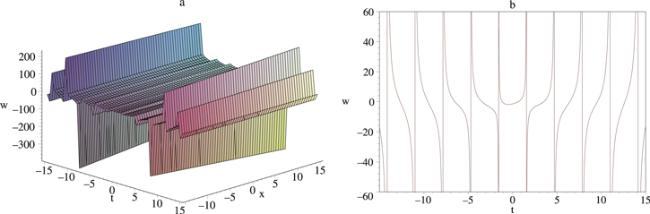
Figure 1. (a) The three-dimensional of the invariant solution at y = 6. (b) The wave-propagation pattern of the wave along t axis at x = 6 and y = 6. |
6. Summary and conclusion
In summary, the Painlevé analysis and the symmetry reductions of the (2+1)-dimensional KdVSKR equation are systematically studied. The Lie group of the KdVSKR equation is the transformations for acting on the independent variables x, y, t and the dependent variables u, w. The symmetry group of the KdVSKR equation is infinite-dimensional due to the existence of three arbitrary functions. The infinite-dimensional Lie groups and Lie algebras, in particular, Kac–Moody–Virasoro algebras are constructed by the Lie point symmetry method. A finite-dimensional subalgebra of physical transformations is studied by selecting first-order polynomials in t. The commutation relations of the subalgebra, which are obtained by selecting the Laurent polynomials in t, have been constructed. From the commutation relations, the symmetry constitutes a centerless Virasoro algebra. Furthermore, symmetry reductions are performed by using the Lie point symmetry method. Three types of similarity reduction equations are studied in the implementation of the method. The Lie point method has generated many reductions and exact solutions in a number of physically important NLPEs [34, 35]. The study of symmetry reductions would be valuable help in work on the nonlinear fields.