


1. Introduction
In a quantum sense, vacuum fluctuates all the time and vacuum fluctuations are responsible for various well-known phenomena, for instance, the interaction potential between two neutral polarizable atoms (molecules) [1–3]. When an atom is perturbed by electromagnetic vacuum fluctuations, an instantaneous electric dipole is induced which then emits a radiative field acting on the other atom, and thus the two atoms are correlated and an interaction potential is resulted. It is now textbook knowledge that the interaction between two inertial atoms in a vacuum is always attractive, and its separation-dependence in the far region L ≫ λ is, due to the effect of retardation, one order higher than that in the near region L ≪ λ, where L and λ are respectively the interatomic separation and the atomic transition wavelength [2]. Usually, the interatomic interactions in the two regions L ≪ λ and L ≫ λ are referred to as the van der Waals (vdW) and the Casimir–Polder (CP) interactions, respectively.
During the past decades, the interatomic interaction has been extensively studied in various circumstances, such as for atoms in a thermal bath [4–12], in synchronous accelerated motion in a vacuum [13, 14], and in the vicinity of boundaries [10, 15, 16]. In almost all aforementioned studies, the potential is analyzed for atoms with almost the same transition frequency and so the role of different frequencies of the atoms is rarely much studied. Although the situation of natural atoms with remarkably different principal transition wavelengths is not very common, there in principle exist some special cases in which the atomic transition wavelengths differ obviously, for example, a hydrogen atom in the vicinity of a Cesium atom, whose first transition wavelengths are respectively ∼1218 Å and ∼8946 Å. Let us note that when two nonidentical atoms with dramatically different transition frequencies ωA ≫ ωB are considered, three rather than two length parameters single out, i.e. L and ${\lambda }_{\xi }=2\pi {\omega }_{\xi }^{-1}$ with ξ = A, B, so that the full region of the interatomic separation L can be divided into three typical regions L ≪ λA ≪ λB, λA ≪ L ≪ λB, and λA ≪ λB ≪ L. Then interesting questions arise as to how the interatomic interaction will behave in different regions. Intuitively, one may anticipate that the interaction in regions L ≪ λA ≪ λB and λA ≪ λB ≪ L behaves similarly to their counterparts in regions L ≪ λ and L ≫ λ in the two-identical-atom case. But for the intermediate region λA ≪ L ≪ λB which does not exist in the two-identical-atom case, one may not be so sure about the answer since there seems to be at least three possibilities: it may exhibit a vdW-like behavior because L ≪ λB, or a CP-like behavior since λA ≪ L, or a new behavior completely distinctive from both the vdW and the CP interactions since L is not simultaneously much smaller or larger than both λA and λB.
In this work, we try to answer these questions by examining the interaction potential of two ground-state atoms with remarkably distinctive transition frequencies. For this purpose, we first consider the potential of two atoms in interaction with a scalar field in a free space and then that of two atoms near an infinite reflecting boundary. Concerning the boundary effects, it is worth re-mentioning that although there have already been some related discussions on the interaction potential of two ground-state atoms in a vacuum near a boundary, i.e. [15, 16], they are incomplete, since the interaction potentials were considered in only a few regions, let alone the role of atomic distinctive transition frequency. In our present work, we will fill this gap by giving a complete discussion for the interaction potential in full regions. As we shall demonstrate, we find some unique behaviors for the interaction potential in both the two-identical-atom and the two-nonidentical-atom cases. To the best of our knowledge, even those results for the two-identical-atom case have never been reported before. We exploit the model of atoms in interaction with a scalar field, which although less realistic as compared with the model of atoms in interaction with an electromagnetic field, helps to reduce, to a large extent, the complexity of calculation and meanwhile still preserves the essential physics as the underlying mechanism of atomic radiative properties in both the scalar and electromagnetic field cases is similar. That is also the reason why it was frequently utilized for the study of atom-field interaction [13, 14, 17–23].
We evaluate the interaction potential with an approach distinctive from those exploited in [15, 16], i.e. the DDC formalism (the formalism proposed by Dalibard, Dupont-Roc and Cohen-Tannoudji) [17, 24, 25], which is a powerful method for the study of radiative properties of atoms in interaction with various quantum fields. The original DDC formalism was established for the study of evolution of a small quantum system in interaction with a large reservoir [24, 25], and then it was widely exploited to study various atomic radiative phenomena, such as the excitation rate and energy shifts of a noninertial atom [18–22, 26, 27] (just to name a few), which are all second-order perturbation effects. Recently, it was generalized from the second order to the fourth order in an attempt to deal with the interaction between two ground-state atoms which is of the fourth order [17]. It was found that the interaction potential is generally ascribed to the contributions of vacuum fluctuations and those of the radiation reaction of the atoms, i.e. the contributions of the free field which exists even when there is no coupling between the atoms and the field and those of the source field which is induced by the atom-field interaction. With this approach, we will show how the interaction potential of two nonidentical atoms has resulted from joint contributions of the vacuum fluctuations and the radiation reaction of atoms, discuss how remarkable discrepancy in the atomic transition frequency affects the interatomic interaction potential, and demonstrate the boundary effects.
The paper is organized as follows. Section 2 is devoted to the interaction potential of two atoms in a free space, for which we first derive general expressions and then analyze in detail the potential in three typical regions. Then in section 3 , we demonstrate the boundary effects by concretely considering the potential of two nonidentical atoms in parallel or vertical alignment to the boundary. The effects of large discrepancy in the atomic transition frequency will also be analyzed detailedly. We give a summary of our work in section 4 . Throughout the paper, we exploit units that ℏ = c = 1.
2. Interatomic interaction potential in a free space
We now consider the interaction potential of two static ground-state atoms A and B in a free space. Assume that the atoms are two-level ones and their ground and excited states are denoted by ∣gξ⟩ and ∣eξ⟩ respectively with ξ = A, B, and then the Hamiltonian of the two-atom system can be expressed as
$\begin{eqnarray}{H}_{S}(t)={\omega }_{A}{R}_{3}^{A}(t)+{\omega }_{B}{R}_{3}^{B}(t)\end{eqnarray}$
with t the coordinate time, ωξ the transition frequency of atom ξ, and ${R}_{3}^{\xi }=\tfrac{1}{2}(| {{e}}_{\xi }\rangle \langle {{e}}_{\xi }| -| {g}_{\xi }\rangle \langle {g}_{\xi }| )$. In a vacuum, the atoms are inevitably perturbed by the fluctuating field $\begin{eqnarray}\phi (x)\equiv \phi (t,{\boldsymbol{x}})=\int {{\rm{d}}}^{3}{\boldsymbol{k}}\ {g}_{{\boldsymbol{k}}}[{a}_{{\boldsymbol{k}}}(t){{\rm{e}}}^{{\rm{i}}{\boldsymbol{k}}\cdot {\boldsymbol{x}}}+{\rm{H}}.{\rm{c}}.],\end{eqnarray}$
where k is the wave vector of field modes, ${g}_{{\boldsymbol{k}}}={\left[2{\omega }_{{\boldsymbol{k}}}{\left(2\pi \right)}^{3}\right]}^{-\tfrac{1}{2}}$, ak denotes the annihilation operator with momentum k, and ‘H.c.' represents the Hermitian conjugate, respectively. Then the Hamiltonian of the scalar field reads $\begin{eqnarray}{H}_{F}(t)=\int {{\rm{d}}}^{3}{\boldsymbol{k}}\ {\omega }_{{\boldsymbol{k}}}{a}_{{\boldsymbol{k}}}^{\dagger }(t){a}_{{\boldsymbol{k}}}(t),\end{eqnarray}$
and that describing the atom-field interaction can be depicted by $\begin{eqnarray}{H}_{I}(t)=\mu {R}_{2}^{A}(t)\phi ({x}_{A})+\mu {R}_{2}^{B}(t)\phi ({x}_{B}),\end{eqnarray}$
where μ is a small coupling constant, ${R}_{2}^{\xi }=\tfrac{{\rm{i}}}{2}({R}_{-}^{\xi }-{R}_{+}^{\xi })$ is the monopole moment operator of atom ξ with ${R}_{+}^{\xi }=| {{e}}_{\xi }\rangle \langle {g}_{\xi }| $ and ${R}_{-}^{\xi }=| {g}_{\xi }\rangle \langle {{e}}_{\xi }| $.As a result of the interaction between the atoms and the field, each atom is endowed with a monopole and meanwhile emits a radiative field superimposed on the free field which exists even when there is no coupling between the atoms and the field, and thus both the free and the atomic radiative fields contribute to the interatomic interaction. As we have mentioned in the introduction, the fourth-order DDC formalism [17] provides a general framework to evaluate the interaction potential by separately calculating the contributions of the free field and those of the atomic radiative field. Here we evaluate the interatomic interaction potential in that way.
2.1. General results
Following [17] and as we have detailedly demonstrated in appendix A.1 , we first derive the symmetric correlation function and linear susceptibility of the field at the two positions of the atoms as well as the two statistical functions of the atoms, use them in the basic formulas describing the vf- and rr-contributions (equations (64) and (66) of [17]), do some simplifications, and then obtain
$\begin{eqnarray}\begin{array}{l}{\left(\delta E\right)}_{\mathrm{vf}}^{(0)}=-\displaystyle \frac{{\mu }^{4}\left[{\omega }_{B}\cos \left(2{\omega }_{A}L\right)-{\omega }_{A}\cos \left(2{\omega }_{B}L\right)\right]}{512{\pi }^{2}{L}^{2}\left({\omega }_{A}^{2}-{\omega }_{B}^{2}\right)}\\ \quad -\displaystyle \frac{{\mu }^{4}{\omega }_{A}{\omega }_{B}}{256{\pi }^{3}{L}^{2}}{\int }_{0}^{\infty }{\rm{d}}u\displaystyle \frac{{{\rm{e}}}^{-2{uL}}}{({\omega }_{A}^{2}+{u}^{2})({\omega }_{B}^{2}+{u}^{2})},\end{array}\end{eqnarray}$
$\begin{eqnarray}\begin{array}{l}{\left(\delta E\right)}_{\mathrm{rr}}^{(0)}=\displaystyle \frac{{\mu }^{4}\left[{\omega }_{B}\cos \left(2{\omega }_{A}L\right)-{\omega }_{A}\cos \left(2{\omega }_{B}L\right)\right]}{512{\pi }^{2}{L}^{2}\left({\omega }_{A}^{2}-{\omega }_{B}^{2}\right)}\\ \quad -\displaystyle \frac{{\mu }^{4}{\omega }_{A}{\omega }_{B}}{256{\pi }^{3}{L}^{2}}{\int }_{0}^{\infty }{\rm{d}}u\displaystyle \frac{{{\rm{e}}}^{-2{uL}}}{({\omega }_{A}^{2}+{u}^{2})({\omega }_{B}^{2}+{u}^{2})},\end{array}\end{eqnarray}$
which are the contributions of the free field in vacuum (vf-contribution) and those of the radiation reaction of the atoms (rr-contribution), respectively. The total interaction potential is then given by the sum of the two contributions $\begin{eqnarray}{\left(\delta E\right)}_{\mathrm{tot}}^{(0)}=-\displaystyle \frac{{\mu }^{4}{\omega }_{A}{\omega }_{B}}{128{\pi }^{3}{L}^{2}}{\int }_{0}^{\infty }{\rm{d}}u\ \displaystyle \frac{{{\rm{e}}}^{-2{uL}}}{({\omega }_{A}^{2}+{u}^{2})({\omega }_{B}^{2}+{u}^{2})}.\quad \end{eqnarray}$
The above equation is the general expression of the total interaction potential of two nonidentical atoms with an arbitrary separation L in a free space while equations (5 ) and (6 ) are those of the vf- and rr-contribution to it. Obviously, although both the vf- and the rr-contributions contain oscillatory terms with respect to L, the total interaction potential exhibits a monotonic decreasing behavior with the increase of L, as a result of the perfect cancellation of oscillatory terms in ${\left(\delta E\right)}_{\mathrm{vf}}^{(0)}$ and ${\left(\delta E\right)}_{\mathrm{rr}}^{(0)}$. In addition, equation (7 ) suggests that the total interaction potential is always negative.
Further simplifications of these results with general values of L are formidable, however, we can still obtain some simple analytical results in some limiting cases which are of particular physical interest, i.e. regions where the interatomic separation L is much smaller or larger than the transition wavelengths of the atoms ${\lambda }_{\xi }=2\pi {\omega }_{\xi }^{-1}$. In the following, we assume ωA ≫ ωB and then the three characteristic lengths L, λA and λB in this problem naturally divide the full region of L into three typical regions, i.e. L ≪ λA ≪ λB, λA ≪ L ≪ λB, and λA ≪ λB ≪ L. We next first analyze the interaction potentials in the two regions L ≪ λA ≪ λB and λA ≪ λB ≪ L which reduce to the vdW region L ≪ λ and the CP region L ≫ λ for two identical atoms with the same transition wavelength λ, and then the region λA ≪ L ≪ λB which does not exist for two identical atoms.
2.2. Interaction potential in limiting cases
When L ≪ λA ≪ λB, we find that equations (5 ) and (6 ) are approximated by8 ) and (9 ) is characterized by the coefficient c1 or c2 closely related to ρ.
$\begin{eqnarray}{\left(\delta E\right)}_{\mathrm{vf}}^{(0)}\simeq \displaystyle \frac{{\mu }^{4}{c}_{1}}{256{\pi }^{3}L},\end{eqnarray}$
$\begin{eqnarray}{\left(\delta E\right)}_{\mathrm{rr}}^{(0)}\simeq -\displaystyle \frac{{\mu }^{4}{c}_{2}}{512{\pi }^{2}\omega {L}^{2}}+\displaystyle \frac{{\mu }^{4}{c}_{1}}{256{\pi }^{3}L},\end{eqnarray}$
with ${c}_{1}=\tfrac{2\mathrm{ln}\rho }{\rho }$ and ${c}_{2}=2\left(\tfrac{1}{\rho }-\tfrac{1}{{\rho }^{2}}\right)$. Hereafter, we abbreviate ωB by ω and introduce a new parameter $\rho =\tfrac{{\omega }_{A}}{\omega }\gg 1$. These results show that the leading-order vf-contribution and the subleading-order rr-contribution are identical and they scale as L−1, while the leading-order rr-contribution scales as L−2, which are qualitatively the same as their counterparts in the two-identical-atom case (see equations (5) and (6) of [14]). However, quantitatively speaking, their strengths are altered due to the discrepancy in the atomic transition frequency, since every term in equations (Comparing the absolute values of the above ${\left(\delta E\right)}_{\mathrm{vf}}^{(0)}$ and ${\left(\delta E\right)}_{\mathrm{rr}}^{(0)}$, we find that $| {\left(\delta E\right)}_{\mathrm{rr}}^{(0)}| \gg | {\left(\delta E\right)}_{\mathrm{vf}}^{(0)}| $, which is qualitatively similar to those of two identical atoms in a free space, and thus
$\begin{eqnarray}{\left(\delta E\right)}_{\mathrm{tot}}^{(0)}\simeq {\left(\delta E\right)}_{\mathrm{rr}}^{(0)}\simeq -\displaystyle \frac{{\mu }^{4}{c}_{2}}{512{\pi }^{2}\omega {L}^{2}},\end{eqnarray}$
which exhibits the L−2-dependence and is c2 times of that of two identical ones with the transition frequency ω.When λA ≪ λB ≪ L, equations (5 ) and (6 ) reduce to
$\begin{eqnarray}\begin{array}{rcl}{\left(\delta E\right)}_{\mathrm{vf}}^{(0)} & \simeq & \displaystyle \frac{{\mu }^{4}[{c}_{3}\cos (2\omega L)-{c}_{3}^{2}\cos (2\rho \omega L)]}{512{\pi }^{2}\omega {L}^{2}}\\ & & -\displaystyle \frac{{\mu }^{4}{c}_{3}}{512{\pi }^{3}{\omega }^{2}{L}^{3}},\end{array}\end{eqnarray}$
$\begin{eqnarray}\begin{array}{rcl}{\left(\delta E\right)}_{\mathrm{rr}}^{(0)} & \simeq & -\displaystyle \frac{{\mu }^{4}[{c}_{3}\cos (2\omega L)-{c}_{3}^{2}\cos (2\rho \omega L)]}{512{\pi }^{2}\omega {L}^{2}}\\ & & -\displaystyle \frac{{\mu }^{4}{c}_{3}}{512{\pi }^{3}{\omega }^{2}{L}^{3}},\end{array}\end{eqnarray}$
with ${c}_{3}=\tfrac{1}{\rho }$. Obviously, both ${\left(\delta E\right)}_{\mathrm{vf}}^{(0)}$ and ${\left(\delta E\right)}_{\mathrm{rr}}^{(0)}$ contain oscillatory and non-oscillatory terms, and they solely oscillate obviously with L, since the amplitudes of oscillatory terms are much greater than absolute values of the non-oscillatory terms. These oscillation behaviors remind us that both the vf- and rr-contributions to the interaction potential of two identical atoms in the region L ≫ λ, as shown in equations (8) and (9) of [14], also oscillate obviously with L. However, the oscillation behaviors in these two cases are distinctive in that here the amplitude of oscillation for two nonidentical atoms scales as L−2, while that for two identical atoms scales as L−1, suggesting that dramatic discrepancy in the atomic transition frequency leads to an obvious change for the sole oscillation behavior of the vf- and rr-contributions. This change, however, does not carry onto the total interaction potential due to the perfect cancellation of oscillatory terms from both the vf- and rr-contributions, and thus we have $\begin{eqnarray}{\left(\delta E\right)}_{\mathrm{tot}}^{(0)}\simeq -\displaystyle \frac{{\mu }^{4}{c}_{3}}{256{\pi }^{3}{\omega }^{2}{L}^{3}},\end{eqnarray}$
which shows the L−3-dependence one order higher than that in the near region L ≪ λA ≪ λB. This phenomenon is a result of retardation and it also happens in the two-identical-atom case, i.e. the interaction potential of two identical atoms in regions L ≪ λ and L ≫ λ also respectively displays the L−2- and L−3-dependence. However, despite this similarity, let us note that the strength of this potential for two nonidentical atoms, as compared with that of two identical ones, is modified by the coefficient c3 characterizing the discrepancy in the atomic transition frequency.Now let us turn our attention to the interaction potential in the region λA ≪ L ≪ λB which does not exist for the two-identical-atom case. We find that when λA ≪ L ≪ λB, equations (5 ) and (6 ) are respectively simplified into
$\begin{eqnarray}{\left(\delta E\right)}_{\mathrm{vf}}^{(0)}\simeq -\displaystyle \frac{{\mu }^{4}{c}_{3}\mathrm{ln}\left(\omega L\right)}{128{\pi }^{3}L},\end{eqnarray}$
$\begin{eqnarray}{\left(\delta E\right)}_{\mathrm{rr}}^{(0)}\simeq -\displaystyle \frac{{\mu }^{4}{c}_{3}}{256{\pi }^{2}\omega {L}^{2}}-\displaystyle \frac{{\mu }^{4}{c}_{3}\mathrm{ln}\left(\omega L\right)}{128{\pi }^{3}L}.\end{eqnarray}$
Obviously, the separation-dependence of these results is very different from those in the far region λA ≪ λB ≪ L; while they resemble, to some extent, those in the near region L ≪ λA ≪ λB (equations (8 ) and (9 )) in the sense that both the vf-contribution in the present region and that in L ≪ λA ≪ λB lead to a positive potential although the separation-dependences in two regions are not identical, the leading terms of the rr-contributions in both regions are identical, and the rr-contribution dominates over the vf-contribution. As a result, the total potential which mainly comes from the rr-contribution is approximated by
$\begin{eqnarray}{\left(\delta E\right)}_{\mathrm{tot}}^{(0)}\simeq -\displaystyle \frac{{\mu }^{4}{c}_{3}}{256{\pi }^{2}\omega {L}^{2}}-\displaystyle \frac{{\mu }^{4}{c}_{3}\mathrm{ln}\left(\omega L\right)}{64{\pi }^{3}L}.\end{eqnarray}$
This potential in the leading order is identical to that in the near region L ≪ λA ≪ λB, and distinctions in the total interaction potential in these two regions appear from the subleading order (see equations (8 ) and (9 )). Further comparing this result with equations (10 ) and (13 ), it is obvious that retardation for the interaction potential of two nonidentical atoms never appears in the region λA ≪ L ≪ λB; it shows up only when the interatomic separation is much larger than the transition wavelengths of both atoms.
So far, we have analyzed the interaction potential of two nonidentical atoms in a free space. We next focus on that of two atoms near a boundary.
3. Interatomic interaction potential near a boundary
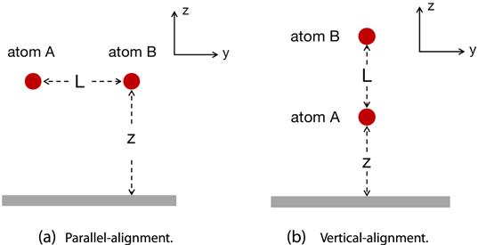
As shown in figure 1, we now consider the interaction potential of two nonidentical atoms A and B fixed near a perfectly reflecting boundary in two different configurations, i.e. atoms aligned with a separation L parallel (‘∥') or perpendicular (‘⊥') to the boundary.
Figure 1. Sketch of two static atoms in parallel or vertical alignment with respect to an infinite boundary. |
Following similar procedures as we demonstrated in section 2 and appendix A.2 , we find that the vf- and rr-contributions to the interaction potential of the two atoms near the boundary can be expressed as a sum of their counterparts in a free space ${\left(\delta E\right)}_{\mathrm{vf},\mathrm{rr}}^{(0)}$ and other terms crucially dependent on the relative position of the two-atom system to the boundary and denoted by ${\left(\delta E\right)}_{\mathrm{vf},\mathrm{rr}}^{\alpha ,(b)}$, i.e.
$\begin{eqnarray}{\left(\delta E\right)}_{\mathrm{vf},\mathrm{rr}}^{\alpha }={\left(\delta E\right)}_{\mathrm{vf},\mathrm{rr}}^{(0)}+{\left(\delta E\right)}_{\mathrm{vf},\mathrm{rr}}^{\alpha ,(b)}\end{eqnarray}$
with $\begin{eqnarray}\begin{array}{rcl}{\left(\delta E\right)}_{\mathrm{vf}}^{\alpha ,(b)} & = & \displaystyle \frac{{\mu }^{4}{H}_{+}({\omega }_{A},{\omega }_{B},{R}_{\alpha })}{512{\pi }^{2}{R}_{\alpha }^{2}}\\ & & -\displaystyle \frac{{\mu }^{4}{H}_{+}\left({\omega }_{A},{\omega }_{B},\tfrac{L+{R}_{\alpha }}{2}\right)}{256{\pi }^{2}{{LR}}_{\alpha }},\end{array}\end{eqnarray}$
$\begin{eqnarray}\begin{array}{rcl}{\left(\delta E\right)}_{\mathrm{rr}}^{\alpha ,(b)} & = & \displaystyle \frac{{\mu }^{4}{H}_{-}({\omega }_{A},{\omega }_{B},{R}_{\alpha })}{512{\pi }^{2}{R}_{\alpha }^{2}}\\ & & -\displaystyle \frac{{\mu }^{4}{H}_{-}\left({\omega }_{A},{\omega }_{B},\tfrac{L+{R}_{\alpha }}{2}\right)}{256{\pi }^{2}{{LR}}_{\alpha }}.\end{array}\end{eqnarray}$
Here α = ∥ or ⊥ is introduced to identify the two distinctive alignments, ${R}_{\parallel }=\sqrt{{L}^{2}+4{z}^{2}}$, R⊥ = (L + 2z), and
$\begin{eqnarray}\begin{array}{l}{H}_{\pm }({\omega }_{A},{\omega }_{B},s)=\mp \displaystyle \frac{{\omega }_{B}\cos \left(2{\omega }_{A}s\right)-{\omega }_{A}\cos \left(2{\omega }_{B}s\right)}{{\omega }_{A}^{2}-{\omega }_{B}^{2}}\\ \quad -\displaystyle \frac{2}{\pi }{\int }_{0}^{\infty }{\rm{d}}u\ \displaystyle \frac{{\omega }_{A}{\omega }_{B}{{\rm{e}}}^{-2{us}}}{({\omega }_{A}^{2}+{u}^{2})({\omega }_{B}^{2}+{u}^{2})}.\end{array}\end{eqnarray}$
Hereafter, z denotes the separation between the boundary and the atoms in the parallel-alignment case or the separation between the boundary and the atom closer to the boundary (atom A) in the vertical-alignment case. Then the total interaction potential follows
$\begin{eqnarray}{\left(\delta E\right)}_{\mathrm{tot}}^{\alpha }={\left(\delta E\right)}_{\mathrm{tot}}^{(0)}+{\left(\delta E\right)}_{\mathrm{tot}}^{\alpha ,(b)}\end{eqnarray}$
with ${\left(\delta E\right)}_{\mathrm{tot}}^{(0)}$ the total interaction potential of two atoms in a free space and $\begin{eqnarray}\begin{array}{l}{\left(\delta E\right)}_{\mathrm{tot}}^{\alpha ,(b)}=\displaystyle \frac{{\mu }^{4}{\omega }_{A}{\omega }_{B}}{64{\pi }^{3}{{LR}}_{\alpha }}{\int }_{0}^{\infty }\quad {\rm{d}}u\\ \quad \,\times \displaystyle \frac{{{\rm{e}}}^{-u(L+{R}_{\alpha })}-\tfrac{L}{2{R}_{\alpha }}{{\rm{e}}}^{-2{{uR}}_{\alpha }}}{({\omega }_{A}^{2}+{u}^{2})({\omega }_{B}^{2}+{u}^{2})}\end{array}\end{eqnarray}$
boundary-induced modifications. Now one can easily judge that there are four characteristic lengths in this problem, i.e. L, ${\lambda }_{\xi }=2\pi {\omega }_{\xi }^{-1}$ with ξ = A, B, and z. Since the above expressions are generally difficult to simplify, we next analyze them in some limited cases. Similar to the previous section, we still assume that λA ≪ λB, then the four parameters L, λA, λB, and z divide the full region of L into twelve regions. As we shall demonstrate, the potentials in some of these regions, as compared with that in a free space, are slightly modified while those in the other regions are severely altered.3.1. Weak effects of the boundary
We find that the total interaction potential of the two nonidentical atoms as well as the vf- and rr-contributions to it are slightly modified in both the parallel- and vertical-alignment cases when L ≪ z, i.e. when the interatomic separation is much smaller than z characterizing the relative position of the two-atom system to the boundary. Particularly when z and λξ further satisfy z ≫ λξ, the modifications in the total interaction potential equally come from the vf- and rr-contributions; while if z is much smaller than at least one of λA and λB, they mainly come from the rr-contribution.
3.1.1. Slight modifications equally from the vf- and rr-contribution
When L ≪ λA ≪ λB ≪ z or λA ≪ L ≪ λB ≪ z or λA ≪ λB ≪ L ≪ z, the boundary induces slight modifications for both the vf- and rr-contributions to the interaction potential of atoms in both the parallel- and vertical-alignment cases, i.e. ${\left(\delta E\right)}_{\mathrm{vf},\mathrm{rr}}^{\alpha ,(b)}\ll {\left(\delta E\right)}_{\mathrm{vf},\mathrm{rr}}^{(0)}$. And to the leading order, they are identical in the two alignment cases, i.e.
$\begin{eqnarray}\begin{array}{rcl}{\left(\delta E\right)}_{\mathrm{vf}}^{\alpha ,(b)} & \simeq & -\displaystyle \frac{{\mu }^{4}[{c}_{3}\cos (2\omega z)-{c}_{3}^{2}\cos (2\rho \omega z)]}{512{\pi }^{2}\omega {zL}}\\ & & +\displaystyle \frac{{\mu }^{4}{c}_{3}}{512{\pi }^{3}{\omega }^{2}{z}^{2}L},\end{array}\end{eqnarray}$
$\begin{eqnarray}\begin{array}{rcl}{\left(\delta E\right)}_{\mathrm{rr}}^{\alpha ,(b)} & \simeq & \displaystyle \frac{{\mu }^{4}[{c}_{3}\cos (2\omega z)-{c}_{3}^{2}\cos (2\rho \omega z)]}{512{\pi }^{2}\omega {zL}}\\ & & +\displaystyle \frac{{\mu }^{4}{c}_{3}}{512{\pi }^{3}{\omega }^{2}{z}^{2}L},\end{array}\end{eqnarray}$
which manifest obvious oscillation behaviors with respect to z. Since the amplitudes of oscillatory terms in these two equations are much greater than the non-oscillatory terms, both ${\left(\delta E\right)}_{\mathrm{vf}}^{\alpha ,(b)}$ and ${\left(\delta E\right)}_{\mathrm{rr}}^{\alpha ,(b)}$ can be positive or negative and even null, depending on the concrete values of ρ and z, suggesting that both the vf- and rr-contributions can either be enhanced or weakened or even unaltered by the presence of the boundary. However, their joint contribution leads to a non-oscillatory modification, i.e. $\begin{eqnarray}{\left(\delta E\right)}_{\mathrm{tot}}^{\alpha ,(b)}\simeq \displaystyle \frac{{\mu }^{4}{c}_{3}}{256{\pi }^{3}{\omega }^{2}{z}^{2}L}.\end{eqnarray}$
Noteworthily, this modification is positive, while the interaction potential in a free space ${\left(\delta E\right)}_{\mathrm{tot}}^{(0)}$ is definitely negative with the absolute value much larger (see equations (10 ), (13 ) and (16 )), and thus the presence of the boundary in these regions only slightly weakens the interaction between the two nonidentical atoms.
The above results are about the interaction potential of two nonidentical atoms with remarkably distinct frequencies. Then does there exist any essential differences between this potential and that of two identical atoms? Note that the region λA ≪ L ≪ λB ≪ z makes no sense for two identical atoms, while the other two regions L ≪ λA ≪ λB ≪ z and λA ≪ λB ≪ L ≪ z for two nonidentical atoms respectively correspond to L ≪ λ ≪ z and λ ≪ L ≪ z for two identical ones, in which the boundary-induced modifications for the vf- and rr-contributions are
$\begin{eqnarray}{\left(\overline{\delta E}\right)}_{\mathrm{vf}}^{\alpha ,(b)}\approx -\displaystyle \frac{{\mu }^{4}\sin (2\omega z+\theta )}{512{\pi }^{2}L}+\displaystyle \frac{{\mu }^{4}}{512{\pi }^{3}{\omega }^{2}{z}^{2}L},\end{eqnarray}$
$\begin{eqnarray}{\left(\overline{\delta E}\right)}_{\mathrm{rr}}^{\alpha ,(b)}\approx \displaystyle \frac{{\mu }^{4}\sin (2\omega z+\theta )}{512{\pi }^{2}L}+\displaystyle \frac{{\mu }^{4}}{512{\pi }^{3}{\omega }^{2}{z}^{2}L}\end{eqnarray}$
with $\theta =\arcsin {\left(\sqrt{1+4{\omega }^{2}{z}^{2}}\right)}^{-1}$. Hereafter, $\overline{\delta E}$ refers to the interaction potential of two identical atoms. Similar to those for two nonidentical atoms, both ${\left(\overline{\delta E}\right)}_{\mathrm{vf}}^{\alpha ,(b)}$ and ${\left(\overline{\delta E}\right)}_{\mathrm{rr}}^{\alpha ,(b)}$ oscillate with z, and the amplitudes of the oscillatory terms are much larger than the non-oscillatory terms. However, different from those in the two-nonidentical-atom case, here the amplitudes of oscillatory terms in the two-identical-atom case are independent of the atomic frequency ω and the parameter z characterizing the relative position between the atom-system and the boundary. This distinction suggests that dramatic discrepancy in the atomic transition frequency can also change the oscillation behaviors of both the vf- and rr-contributions when two atoms are near a boundary.Adding the above two equations up, we obtain25 )). And in comparison, boundary-induced modifications for the total interaction potential of two nonidentical atoms in region L ≪ λA ≪ λB ≪ z or λA ≪ L ≪ λB ≪ z or λA ≪ λB ≪ L ≪ z, as demonstrated by equation (25 ), is ${c}_{3}=\tfrac{1}{\rho }$ times of that of two identical ones with frequency ω in regions L ≪ λ ≪ z and λ ≪ L ≪ z, i.e. remarkable discrepancy in the atomic transition frequency rescales the strength of boundary-induced modifications for the total interaction potential but never changes its separation-dependence.
$\begin{eqnarray}{\left(\overline{\delta E}\right)}_{\mathrm{tot}}^{\alpha ,(b)}\approx \displaystyle \frac{{\mu }^{4}}{256{\pi }^{3}{\omega }^{2}{z}^{2}L},\end{eqnarray}$
which is the boundary-induced modification for the total interaction potential of two identical atoms, exhibiting the same monotonic separation-dependence of L−1 as that of the interaction potential of two nonidentical atoms in a free space (see equation (3.1.2. Slight modifications mainly from the rr-contribution
We find that when L ≪ λA ≪ z ≪ λB or L ≪ z ≪ λA ≪ λB or λA ≪ L ≪ z ≪ λB, the vf-contributions in the leading order behave quite the same in both the parallel- or vertical-alignment cases and they are all z-dependent:
$\begin{eqnarray}{\left(\delta E\right)}_{\mathrm{vf}}^{\alpha }\simeq \left\{\begin{array}{ll}\displaystyle \frac{{\mu }^{4}{c}_{3}\mathrm{ln}(\rho \omega z)}{128{\pi }^{3}L}, & L\ll {\lambda }_{A}\ll z\ll {\lambda }_{B},\\ \displaystyle \frac{{\mu }^{4}\rho {\omega }^{2}{z}^{2}\mathrm{ln}(\rho \omega z)}{192{\pi }^{3}L}, & L\ll z\ll {\lambda }_{A}\ll {\lambda }_{B},\\ \displaystyle \frac{{\mu }^{4}{c}_{3}\mathrm{ln}(\tfrac{z}{L})}{128{\pi }^{3}L}, & {\lambda }_{A}\ll L\ll z\ll {\lambda }_{B},\end{array}\right.\end{eqnarray}$
which in regions L ≪ λA ≪ z ≪ λB and λA ≪ L ≪ z ≪ λB are partly from ${\left(\delta E\right)}_{\mathrm{vf}}^{(0)}$ and partly from ${\left(\delta E\right)}_{\mathrm{vf}}^{\alpha ,(b)}$, while in region L ≪ z ≪ λA ≪ λB is actually the leading-order z-dependent term of ${\left(\delta E\right)}_{\mathrm{vf}}^{\alpha ,(b)}$ which is singled out since those stronger z-independent terms in ${\left(\delta E\right)}_{\mathrm{vf}}^{(0)}$ and ${\left(\delta E\right)}_{\mathrm{vf}}^{\alpha ,(b)}$ cancel out completely. The rr-contribution to the leading order is, however, not altered by the presence of the boundary, i.e. ${\left(\delta E\right)}_{\mathrm{rr}}^{\alpha ,(b)}\ll {\left(\delta E\right)}_{\mathrm{rr}}^{(0)}$, and boundary-induced modifications for it in the three regions are identical in the leading order with distinctions showing up at the subleading order: $\begin{eqnarray}{\left(\delta E\right)}_{\mathrm{rr}}^{\alpha }\simeq -\displaystyle \frac{{\mu }^{4}{c}_{3}}{256{\pi }^{2}\omega {L}^{2}}+\displaystyle \frac{{\mu }^{4}{c}_{3}}{256{\pi }^{2}\omega {zL}}.\end{eqnarray}$
Notice that here the second term is the leading-order ${\left(\delta E\right)}_{\mathrm{rr}}^{\alpha ,(b)}$, which behaves quite the same in three regions, in sharp contrast to the leading-order ${\left(\delta E\right)}_{\mathrm{vf}}^{\alpha ,(b)}$ behaving distinctively in the three regions (see equation (29 )).
Comparing the absolute value of equation (30 ) with that of equation (29 ), one finds that the former is much greater, and thus the total interaction potential is approximated by
$\begin{eqnarray}{\left(\delta E\right)}_{\mathrm{tot}}^{\alpha }\simeq {\left(\delta E\right)}_{\mathrm{rr}}^{\alpha }\simeq -\displaystyle \frac{{\mu }^{4}{c}_{3}}{256{\pi }^{2}\omega {L}^{2}}+\displaystyle \frac{{\mu }^{4}{c}_{3}}{256{\pi }^{2}\omega {zL}}.\end{eqnarray}$
So, as a result of the presence of the boundary, the interaction potential of two nonidentical atoms in regions L ≪ λA ≪ z ≪ λB, L ≪ z ≪ λA ≪ λB, and λA ≪ L ≪ z ≪ λB is slightly weakened with modifications mainly from the rr-contribution.
At the end of this subsection, it is worth pointing out that although the leading-order ${\left(\delta E\right)}_{\mathrm{vf}}^{\alpha ,(b)}$ and ${\left(\delta E\right)}_{\mathrm{rr}}^{\alpha ,(b)}$ for two nonidentical atoms, as we have shown in equations (23 ), (24 ), (29 ), and (30 ), are identical in every region we have sofar considered for both the parallel- and vertical-alignment cases, i.e. regions L ≪ λA ≪ λB ≪ z, λA ≪ L ≪ λB ≪ z, λA ≪ λB ≪ L ≪ z, L ≪ λA ≪ z ≪ λB, L ≪ z ≪ λA ≪ λB and λA ≪ L ≪ z ≪ λB, they actually differ in higher orders. As we shall show in the next subsection, things become quite different in the other six regions where boundary-induced modifications become very important, and distinctions in ${\left(\delta E\right)}_{\mathrm{vf}}^{\alpha ,(b)}$ and ${\left(\delta E\right)}_{\mathrm{rr}}^{\alpha ,(b)}$ in two alignment cases exist even in the leading order.
3.2. Strong effects of the boundary
We find that when z ≪ L, i.e. when the separation between the two-atom system and the boundary is much smaller than the interatomic separation, the boundary induces remarkable modifications for the interaction potential. As a result, the total potential in the leading order is z-dependent, and it should be mainly attributed to the rr-contribution if L is further much smaller than at least one of λA and λB, and to equal vf- and rr-contributions if L is much larger than both λA and λB.
3.2.1. Remarkable modifications mainly from the rr-contribution
When the atoms are in parallel alignment to the boundary in region z ≪ L ≪ λA ≪ λB or λA ≪ z ≪ L ≪ λB or z ≪ λA ≪ L ≪ λB, the vf-contribution in the leading order behaves differently in three regions as
$\begin{eqnarray}{\left(\delta E\right)}_{\mathrm{vf}}^{\parallel }\simeq \left\{\begin{array}{ll}\displaystyle \frac{{\mu }^{4}\rho {\omega }^{2}{z}^{4}}{96{\pi }^{3}{L}^{3}}\mathrm{ln}\left(\rho \omega L\right), & z\ll L\ll {\lambda }_{A}\ll {\lambda }_{B},\\ \displaystyle \frac{3{\mu }^{4}{z}^{4}}{128{\pi }^{3}\rho {L}^{5}}, & {\lambda }_{A}\ll z\ll L\ll {\lambda }_{B},\\ \displaystyle \frac{3{\mu }^{4}{z}^{4}}{128{\pi }^{3}\rho {L}^{5}}\left[1-\displaystyle \frac{\pi \rho \omega L}{3}\sin (2\rho \omega L-\phi )\right], & z\ll {\lambda }_{A}\ll L\ll {\lambda }_{B}\end{array}\right.\end{eqnarray}$
with $\phi =\arctan \left(\tfrac{\rho \omega L}{2}\right)$, and it leads to an attractive interaction force in the first region z ≪ L ≪ λA ≪ λB, a repulsive force in the second region λA ≪ z ≪ L ≪ λB, and either attractive or repulsive force in the third region z ≪ λA ≪ L ≪ λB. The rr-contribution in the leading order in these three regions, however, behaves quite the same as $\begin{eqnarray}{\left(\delta E\right)}_{\mathrm{rr}}^{\parallel }\simeq -\displaystyle \frac{{\mu }^{4}{c}_{3}{z}^{4}}{64{\pi }^{2}\omega {L}^{6}},\end{eqnarray}$
and it is much greater than ${\left(\delta E\right)}_{\mathrm{vf}}^{\parallel }$. As a result, the interaction potential in these three regions should be mainly ascribed to the rr-contribution, and thus we have $\begin{eqnarray}{\left(\delta E\right)}_{\mathrm{tot}}^{\parallel }\simeq {\left(\delta E\right)}_{\mathrm{rr}}^{\parallel }\simeq -\displaystyle \frac{{\mu }^{4}{c}_{3}{z}^{4}}{64{\pi }^{2}\omega {L}^{6}}.\end{eqnarray}$
As compared to $-\tfrac{{\mu }^{4}{c}_{3}}{256{\pi }^{2}\omega {L}^{2}}$, which is the leading-order interaction potential of two atoms in region L ≪ λA ≪ λB or λA ≪ L ≪ λB in a free space, this potential of two atoms near a boundary is much weaker. Particularly, when the atoms are located in regions z ≪ L ≪ λA ≪ λB and z ≪ λA ≪ L ≪ λB and if z → 0, this interaction is vanishingly small. This is physically understandable: since z ∼ 0 means that the atoms are fixed on the boundary where the field strength is null, the atoms are never perturbed by the field and no radiative field is emitted, thus the correlation between the two atoms cannot be established and the two atoms appear to be isolated from each other.
The above results are about the interaction potential of two atoms in parallel alignment in region z ≪ L ≪ λA ≪ λB or λA ≪ z ≪ L ≪ λB or z ≪ λA ≪ L ≪ λB. Then how about the results in these regions in the vertical-alignment case? We find that both the leading-order vf- and rr-contributions as well as the total interaction potential in the vertical-alignment case are accurately z−2L2 times of their counterparts in the parallel-alignment case (equations (32 )–(34 )), and thus characters of the interaction potential in both cases are qualitatively the same. However, since z−2L2 ≫ 1, the interatomic interaction potential in the vertical-alignment case scales as z2L−4 and it is much stronger than that in the parallel-alignment case.
3.2.2. Remarkable modifications equally from the vf- and rr-contributions
When the two atoms are located in regions where L ≫ z and meanwhile L ≫ λA and L ≫ λB, i.e. λA ≪ λB ≪ z ≪ L or λA ≪ z ≪ λB ≪ L or z ≪ λA ≪ λB ≪ L, boundary-induced modifications are also very remarkable, but the interaction potential is no longer mainly contributed by the radiation reaction of the atoms as we have demonstrated in the previous sub-subsection, but equally contributed by the vacuum fluctuations and the radiation reaction of the atoms. To be specific, if the atoms are in parallel alignment to the boundary, the vf- and rr-contributions are respectively
$\begin{eqnarray}\begin{array}{rcl}{\left(\delta E\right)}_{\mathrm{vf}}^{\parallel } & \simeq & \displaystyle \frac{{\mu }^{4}{z}^{4}\left[{c}_{3}\cos (2\omega L)-{c}_{3}^{2}\cos (2\rho \omega L)\right]}{128{\pi }^{2}\omega {L}^{6}}\\ & & -\displaystyle \frac{5{\mu }^{4}{c}_{3}{z}^{4}}{256{\pi }^{3}{\omega }^{2}{L}^{7}},\end{array}\end{eqnarray}$
$\begin{eqnarray}\begin{array}{rcl}{\left(\delta E\right)}_{\mathrm{rr}}^{\parallel } & \simeq & -\displaystyle \frac{{\mu }^{4}{z}^{4}\left[{c}_{3}\cos (2\omega L)-{c}_{3}^{2}\cos (2\rho \omega L)\right]}{128{\pi }^{2}\omega {L}^{6}}\\ & & -\displaystyle \frac{5{\mu }^{4}{c}_{3}{z}^{4}}{256{\pi }^{3}{\omega }^{2}{L}^{7}},\end{array}\end{eqnarray}$
which solely oscillate with the interatomic separation L. However, their summation gives rise to a total interaction potential scaling monotonically with L as $\begin{eqnarray}{\left(\delta E\right)}_{\mathrm{tot}}^{\parallel }\simeq -\displaystyle \frac{5{\mu }^{4}{c}_{3}{z}^{4}}{128{\pi }^{3}{\omega }^{2}{L}^{7}}.\end{eqnarray}$
Note that this L−7-dependence of the interaction potential is sharply different from the ∼L−3-dependence in a free space (equation (13 )), and as compared with the interaction potential in region z ≪ L ≪ λA ≪ λB or λA ≪ z ≪ L ≪ λB or z ≪ λA ≪ L ≪ λB discussed in the previous sub-subsection, it is one order higher, and this is retardation. In addition, let us also point out that here we have only preserved in equation (37 ) the leading-order interaction potential which is identical in three regions, and actually distinctions appear in higher orders.
Now a comparison between this interaction potential of two nonidentical atoms and that of two identical ones is in order. When two identical atoms are considered, the two regions λA ≪ λB ≪ z ≪ L and z ≪ λA ≪ λB ≪ L of two nonidentical atoms reduce to λ ≪ z ≪ L and z ≪ λ ≪ L, where the vf- and rr-contributions are respectively approximated by35 ) and (36 ), while those of non-oscillatory terms are still L−7. So similar to the unbounded case studied in section 2 , here although dramatic discrepancy in the atomic transition frequency obviously modifies the sole oscillatory behaviors of the vf- and rr-contributions in regions where L ≫ z and meanwhile L ≫ λξ, it only alters the strength of the total interaction potential but never changes its separation-dependence, since the oscillatory terms of (δE)vf and (δE)rr are equal in absolute value but opposite in sign (see equations (35 ) and (36 )).
$\begin{eqnarray}{(\overline{\delta E})}_{\mathrm{vf}}\simeq \displaystyle \frac{{\mu }^{4}{z}^{4}\sin (2\omega L+\psi )}{128{\pi }^{2}{L}^{5}}-\displaystyle \frac{5{\mu }^{4}{z}^{4}}{256{\pi }^{3}{\omega }^{2}{L}^{7}},\end{eqnarray}$
$\begin{eqnarray}{(\overline{\delta E})}_{\mathrm{rr}}\simeq -\displaystyle \frac{{\mu }^{4}{z}^{4}\sin (2\omega L+\psi )}{128{\pi }^{2}{L}^{5}}-\displaystyle \frac{5{\mu }^{4}{z}^{4}}{256{\pi }^{3}{\omega }^{2}{L}^{7}}\end{eqnarray}$
with $\psi =\arcsin {\left(\sqrt{1+4{\omega }^{2}{L}^{2}}\right)}^{-1}$. The separation-dependence of the oscillatory terms in the above two equations is quite distinctive from that of two nonidentical atoms displayed in equations (Then how about the interaction potential of two nonidentical atoms in vertical alignment to the boundary in the three regions λA ≪ λB ≪ z ≪ L, λA ≪ z ≪ λB ≪ L and z ≪ λA ≪ λB ≪ L? The answer is that they are qualitatively quite similar to what we have just demonstrated for those of atoms in the parallel-alignment case, i.e. both the vf- and rr-contributions oscillate with L and they solely correspond to an either attractive or repulsive and even vanishing interaction force but jointly give rise to a total interaction potential scaling monotonically with L. However, quantitatively speaking, the interaction potentials in these two alignment cases are distinctive, since37 )), and the former is much stronger. Note also that this L-dependence of the interaction potential in regions λA ≪ λB ≪ z ≪ L, λA ≪ z ≪ λB ≪ L, and z ≪ λA ≪ λB ≪ L in the vertical-alignment case is one order higher than those in regions z ≪ L ≪ λA ≪ λB or λA ≪ z ≪ L ≪ λB or z ≪ λA ≪ L ≪ λB where the interatomic separation L is much smaller than at least one of λA and λB, and this is retardation. This conclusion together with that drawn below equation (37 ) indicates that retardation which happens in a free space also occurs when two atoms are located near a boundary, if the interatomic separation L is much larger than the transition wavelengths of both atoms λA and λB.
$\begin{eqnarray}{\left(\delta E\right)}_{\mathrm{tot}}^{\perp }\simeq -\displaystyle \frac{5{\mu }^{4}{c}_{3}{z}^{2}}{128{\pi }^{3}{\omega }^{2}{L}^{5}},\end{eqnarray}$
which is proportional to z2L−5 while that in the parallel-alignment case is proportional to z4L−7 (see equation (4. Summary
In this paper, we studied the interaction potential of two nonidentical static ground-state atoms A and B with a constant separation L in a free space or in the vicinity of a completely reflecting boundary by calculating the separate contributions of the vacuum fluctuations and the radiation reaction of the atoms. Besides deriving general expressions for the interaction potential of the two atoms in a free space and those of two atoms in parallel or vertical alignment with respect to the boundary, we discussed the interaction potential in detail in various typical regions with special attention paid to the roles of a discrepancy in the atomic transition frequency as well as the presence of the boundary.
Assuming that λA ≪ λB, i.e. the transition wavelength of atom A is much smaller than that of atom B, then for the two atoms in a free space, three characteristic length parameters L, λA, and λB divide the full region of L into three typical regions L ≪ λA ≪ λB, λA ≪ L ≪ λB and λA ≪ λB ≪ L. We found that the separation-dependence of both the vf- and rr-contributions as well as the total interaction potential of the two atoms in region L ≪ λA ≪ λB are the same as their counterparts of two identical atoms in the region L ≪ λ, and the discrepancy in the atomic transition frequency only modifies the strength of the interaction. As a result, the total interaction potential mainly comes from the rr-contribution scales as L−2. In contrast, both the vf- and rr-contributions to the interaction potential of the two atoms in region λA ≪ λB ≪ L which solely oscillate with the interatomic separation L are obviously altered as compared with that of two identical atoms in region λ ≪ L. The total interaction potential which equally comes from the vf- and rr-contributions, however, displays the same L−3-dependence as that of two identical atoms in region L ≫ λ, and it is one order higher than that in the region L ≪ λA ≪ λB. So in this region, the dramatic discrepancy in the atomic transition frequency also only rescales the strength of the total interatomic interaction but never alters its separation-dependence. In the region λA ≪ L ≪ λB which does not exist for two identical atoms, the interaction potential which mainly comes from the rr-contribution behaves in the leading order quite the same as that in the region L ≪ λA ≪ λB, though the leading-order vf-contribution and the subleading-order rr-contribution are obviously distinctive from their counterparts in the region L ≪ λA ≪ λB. These results suggest that retardation for the interaction potential of two nonidentical atoms in a free space appears only when the interatomic separation is much greater than the transition wavelengths of both atoms.
For two atoms near a boundary, we found that boundary-induced modifications are negligible when z ≫ L and remarkable when z ≪ L, with z characterizing the atom-boundary separation in the parallel-alignment case and the separation between the boundary and the atom closer to the boundary (atom A) in the vertical-alignment case. Similar to that in a free space, although a remarkable discrepancy in the atomic transition frequency may lead to obvious change for the sole separation-dependence of the vf- and rr-contribution, it only rescales the strength of the total potential but never alters its separation-dependence.
To be specific, when z ≫ L, the four length parameters L, z, λA, and λB with λA ≪ λB divide the full region of L into six regions which we classify into two sets with the first set including regions L ≪ λA ≪ λB ≪ z, λA ≪ L ≪ λB ≪ z, and λA ≪ λB ≪ L ≪ z, and the second set including L ≪ λA ≪ z ≪ λB, L ≪ z ≪ λA ≪ λB, and λA ≪ L ≪ z ≪ λB. In the first set of regions which are in common that z ≫ L and meanwhile, z is much larger than both λA and λB, boundary-induced modifications for both the vf- and rr-contributions exhibit obvious distinctive oscillation behaviors from those in regions L ≪ λ ≪ z and λ ≪ L ≪ z in the two-identical-atom case, and they equally slightly weaken the interaction potential, as compared with those in a free space. While in the second set of regions which are in common that z ≫ L and z is much smaller than at least one of λA and λB, boundary-induced modifications for the rr-contribution are much larger than those for the vf-contribution, and as a result, the interatomic interaction potential is also slightly weakened as compared with that in a free space. These conclusions are valid for both the parallel- and vertical-alignment cases.
When z ≪ L, the four parameters L, z, λA, and λB with λA ≪ λB also divide the full region of L into two sets of typical regions with z ≪ L ≪ λA ≪ λB, λA ≪ z ≪ L ≪ λB and z ≪ λA ≪ L ≪ λB the first set and λA ≪ λB ≪ z ≪ L, λA ≪ z ≪ λB ≪ L and z ≪ λA ≪ λB ≪ L the second set. We find that in both sets of regions, boundary-induced modifications for both the vf- and rr-contributions in the leading order are z-dependent. As a result, the total interaction potential in the first set of regions mainly comes from the rr-contribution scales as z4L−6 in the parallel-alignment case and as z2L−4 in the vertical-alignment case; while that in the second set which equally comes from the vf- and rr-contributions scales as z4L−7 in the parallel-alignment case and as z2L−5 in the vertical-alignment case. These results suggest that retardation happens for two nonidentical atoms only when the interatomic separation is much greater than both λA and λB.
Appendix. Derivations for the interatomic interaction potential
According to [17], the vf- and rr-contributions to the interaction potential of two static ground-state atoms in vacuum can be expressed as
$\begin{eqnarray}\begin{array}{rcl}{\left(\delta E\right)}_{\mathrm{vf}} & = & 2{\rm{i}}{\mu }^{4}{\int }_{{t}_{0}}^{t}{\rm{d}}{t}_{1}{\int }_{{t}_{0}}^{{t}_{1}}{\rm{d}}{t}_{2}{\int }_{{t}_{0}}^{{t}_{2}}{\rm{d}}{t}_{3}{C}^{F}({x}_{A}(t),{x}_{B}({t}_{3}))\\ & & \times {\chi }^{F}({x}_{A}({t}_{1}),{x}_{B}({t}_{2})){\chi }^{A}(t,{t}_{1}){\chi }^{B}({t}_{2},{t}_{3})+A\iff B\,\mathrm{term}\end{array}\end{eqnarray}$
and $\begin{eqnarray}\begin{array}{l}{\left(\delta E\right)}_{\mathrm{rr}}=2{\rm{i}}{\mu }^{4}{\int }_{{t}_{0}}^{t}{\rm{d}}{t}_{1}{\int }_{{t}_{0}}^{{t}_{1}}{\rm{d}}{t}_{2}{\int }_{{t}_{0}}^{{t}_{2}}{\rm{d}}{t}_{3}\ \\ \times \,{\chi }^{F}({x}_{A}(t),{x}_{B}({t}_{3})){\chi }^{F}({x}_{A}({t}_{1}),{x}_{B}({t}_{2})){C}^{A}(t,{t}_{1}){\chi }^{B}({t}_{2},{t}_{3})\\ +\,2{\rm{i}}{\mu }^{4}{\int }_{{t}_{0}}^{t}{\rm{d}}{t}_{1}{\int }_{{t}_{0}}^{{t}_{1}}{\rm{d}}{t}_{2}{\int }_{{t}_{0}}^{{t}_{2}}{\rm{d}}{t}_{3}\ \\ \times \,{\chi }^{F}({x}_{A}({t}_{1}),{x}_{B}({t}_{3})){\chi }^{F}({x}_{B}({t}_{2}),{x}_{A}(t)){C}^{A}(t,{t}_{1}){\chi }^{B}({t}_{2},{t}_{3})\\ +\,2{\rm{i}}{\mu }^{4}{\int }_{{t}_{0}}^{t}{\rm{d}}{t}_{1}{\int }_{{t}_{0}}^{{t}_{1}}{\rm{d}}{t}_{2}{\int }_{{t}_{0}}^{{t}_{2}}{\rm{d}}{t}_{3}\ \\ \times \,{\chi }^{F}({x}_{A}({t}_{3}),{x}_{B}({t}_{2})){\chi }^{F}({x}_{B}({t}_{1}),{x}_{A}(t)){C}^{A}(t,{t}_{3}){\chi }^{B}({t}_{1},{t}_{2})\\ +\,2{\rm{i}}{\mu }^{4}{\int }_{{t}_{0}}^{t}{\rm{d}}{t}_{1}{\int }_{{t}_{0}}^{t}{\rm{d}}{t}_{2}{\int }_{{t}_{0}}^{{t}_{2}}{\rm{d}}{t}_{3}\ \\ \times \,{\chi }^{F}({x}_{A}({t}_{2}),{x}_{B}({t}_{3})){\chi }^{F}({x}_{A}(t),{x}_{B}({t}_{1})){\chi }^{A}(t,{t}_{2}){C}^{B}({t}_{1},{t}_{3})\\ +\,2{\rm{i}}{\mu }^{4}{\int }_{{t}_{0}}^{t}{\rm{d}}{t}_{1}{\int }_{{t}_{0}}^{{t}_{1}}{\rm{d}}{t}_{2}{\int }_{{t}_{0}}^{t}{\rm{d}}{t}_{3}\ \\ \times \,{C}^{F}({x}_{B}({t}_{2}),{x}_{A}({t}_{3})){\chi }^{F}({x}_{B}({t}_{1}),{x}_{A}(t)){\chi }^{A}({t}_{3},t){\chi }^{B}({t}_{1},{t}_{2})\\ +\,2{\rm{i}}{\mu }^{4}{\int }_{{t}_{0}}^{t}{\rm{d}}{t}_{1}{\int }_{{t}_{0}}^{{t}_{1}}{\rm{d}}{t}_{2}{\int }_{{t}_{0}}^{{t}_{1}}{\rm{d}}{t}_{3}\ \\ \times \,{\chi }^{F}({x}_{A}(t),{x}_{B}({t}_{3})){\chi }^{F}({x}_{A}({t}_{1}),{x}_{B}({t}_{2})){C}^{A}(t,{t}_{1}){\chi }^{B}({t}_{3},{t}_{2})\\ +\,A\iff B\,\mathrm{terms},\end{array}\end{eqnarray}$
where ${C}^{F}({x}_{A}(t),{x}_{B}(t^{\prime} ))$ and ${\chi }^{F}({x}_{A}(t),{x}_{B}(t^{\prime} ))$ are respectively the symmetric correlation function and the linear susceptibility of the field defined as $\begin{eqnarray}{C}^{F}({x}_{A}(t),{x}_{B}(t^{\prime} ))\equiv \displaystyle \frac{1}{2}\langle 0| \{{\phi }^{f}({x}_{A}(t)),{\phi }^{f}({x}_{B}(t^{\prime} ))\}| 0\rangle ,\end{eqnarray}$
$\begin{eqnarray}{\chi }^{F}({x}_{A}(t),{x}_{B}(t^{\prime} ))\equiv \displaystyle \frac{1}{2}\langle 0| [{\phi }^{f}({x}_{A}(t)),{\phi }^{f}({x}_{B}(t^{\prime} ))]| 0\rangle ,\end{eqnarray}$
with ∣0⟩ denoting the vacuum state and $\begin{eqnarray}{\phi }^{f}(x)=\int {{\rm{d}}}^{3}{\boldsymbol{k}}\,{g}_{{\boldsymbol{k}}}[{a}_{{\boldsymbol{k}}}({t}_{0}){{\rm{e}}}^{-{\rm{i}}{\omega }_{{\boldsymbol{k}}}(t-{t}_{0})}{{\rm{e}}}^{{\rm{i}}{\boldsymbol{k}}\cdot {\boldsymbol{x}}}+{\rm{H}}.{\rm{c}}.]\end{eqnarray}$
the free field operator with ${g}_{{\boldsymbol{k}}}={\left[{\left(2\pi \right)}^{3}2{\omega }_{{\boldsymbol{k}}}\right]}^{-1/2}$ and ωk = k, and $\begin{eqnarray}{C}^{\xi }(t,t^{\prime} )\equiv \displaystyle \frac{1}{2}\langle {g}_{\xi }| \{{R}_{2}^{\xi ,f}(t),{R}_{2}^{\xi ,f}(t^{\prime} )\}| {g}_{\xi }\rangle ,\end{eqnarray}$
$\begin{eqnarray}{\chi }^{\xi }(t,t^{\prime} )\equiv \displaystyle \frac{1}{2}\langle {g}_{\xi }| [{R}_{2}^{\xi ,f}(t),{R}_{2}^{\xi ,f}(t^{\prime} )]| {g}_{\xi }\rangle \end{eqnarray}$
are respectively the symmetric and antisymmetric statistical functions of atom ξ with $\begin{eqnarray}{R}_{2}^{\xi ,f}(t)=\displaystyle \frac{{\rm{i}}}{2}[{R}_{-}^{\xi ,f}({t}_{0}){{\rm{e}}}^{-{\rm{i}}{\omega }_{\xi }(t-{t}_{0})}-{R}_{+}^{\xi ,f}({t}_{0}){{\rm{e}}}^{{\rm{i}}{\omega }_{\xi }(t-{t}_{0})}].\end{eqnarray}$
The two statistical functions equations (A6 ) and (A7 ), after the insertion of equation (A8 ), can be further simplified into
$\begin{eqnarray}{C}^{\xi }(t,t^{\prime} )=\displaystyle \frac{1}{8}({{\rm{e}}}^{-{\rm{i}}{\omega }_{\xi }(t-t^{\prime} )}+{{\rm{e}}}^{{\rm{i}}{\omega }_{\xi }(t-t^{\prime} )}),\end{eqnarray}$
$\begin{eqnarray}{\chi }^{\xi }(t,t^{\prime} )=\displaystyle \frac{1}{8}({{\rm{e}}}^{-{\rm{i}}{\omega }_{\xi }(t-t^{\prime} )}-{{\rm{e}}}^{{\rm{i}}{\omega }_{\xi }(t-t^{\prime} )}).\end{eqnarray}$
So to obtain the vf- and rr-contributions, we should first calculate the symmetric correlation function and the linear susceptibility of field ${C}^{F}({x}_{A}(t),{x}_{B}(t^{\prime} ))$ and ${\chi }^{F}({x}_{A}(t),{x}_{B}(t^{\prime} ))$.
A.1. Interaction potential of two atoms in a free space: derivations for equations (5 ) and (6 )
Using equations (A5 ) in (A3 ) and (A4 ) and doing some simplifications, we getA9 )–(A12 ) into (A1 ) and (A2 ), perform the triple integrations with respect to t3, t2 and t1 with the assumption of a sufficiently long time interval t − t0 → ∞ , and we obtain5 ) and (6 ) in section 2 .
$\begin{eqnarray}\begin{array}{rcl}{C}^{F}({x}_{A}(t),{x}_{B}({t}^{{\rm{{\prime} }}})) & = & \displaystyle \frac{1}{8{\pi }^{2}L}{\int }_{0}^{\infty }{\rm{d}}{\omega }^{{\rm{{\prime} }}}{\unicode{x000A0}}\sin ({\omega }^{{\rm{{\prime} }}}L)\\ & \times & ({{\rm{e}}}^{\left.-{\rm{i}}{\omega }^{{\rm{{\prime} }}}(t-{t}^{{\rm{{\prime} }}}\right)}+{{\rm{e}}}^{\left.{\rm{i}}{\omega }^{{\rm{{\prime} }}}(t-{t}^{{\rm{{\prime} }}}\right)}),\end{array}\end{eqnarray}$
$\begin{eqnarray}\begin{array}{l}{\chi }^{F}({x}_{A}(t),{x}_{B}(t^{\prime} ))=\displaystyle \frac{1}{8{\pi }^{2}L}{\int }_{0}^{\infty }{\rm{d}}\omega ^{\prime} \sin (\omega ^{\prime} L)\\ \ \times \,({{\rm{e}}}^{-{\rm{i}}\omega ^{\prime} (t-t^{\prime} )}-{{\rm{e}}}^{{\rm{i}}\omega ^{\prime} (t-t^{\prime} )})\end{array}\end{eqnarray}$
with L the interatomic separation. Now insert equations ( $\begin{eqnarray}\begin{array}{l}{\left(\delta E\right)}_{\mathrm{vf}}^{(0)}=-\displaystyle \frac{{\mu }^{4}{\omega }_{A}{\omega }_{B}}{64{\pi }^{4}{L}^{2}}{\int }_{0}^{\infty }{\rm{d}}{\omega }_{1}{\int }_{0}^{\infty }{\rm{d}}{\omega }_{2}\\ \quad \times \,\displaystyle \frac{{\omega }_{2}\sin ({\omega }_{1}L)\sin ({\omega }_{2}L)}{({\omega }_{1}^{2}-{\omega }_{A}^{2})({\omega }_{1}^{2}-{\omega }_{B}^{2})({\omega }_{2}^{2}-{\omega }_{1}^{2})},\end{array}\end{eqnarray}$
$\begin{eqnarray}\begin{array}{l}{\left(\delta E\right)}_{\mathrm{rr}}^{(0)}=-\displaystyle \frac{{\mu }^{4}}{64{\pi }^{4}{L}^{2}}{\int }_{0}^{\infty }{\rm{d}}{\omega }_{1}{\int }_{0}^{\infty }{\rm{d}}{\omega }_{2}\\ \quad \times \,\displaystyle \frac{{\omega }_{2}[2{\omega }_{1}^{3}-2{\omega }_{1}({\omega }_{A}^{2}+{\omega }_{A}{\omega }_{B}+{\omega }_{B}^{2})+{\omega }_{A}{\omega }_{B}({\omega }_{A}+{\omega }_{B})]}{({\omega }_{A}+{\omega }_{B})({\omega }_{1}^{2}-{\omega }_{A}^{2})({\omega }_{1}^{2}-{\omega }_{B}^{2})({\omega }_{2}^{2}-{\omega }_{1}^{2})}\\ \quad \times \,\sin ({\omega }_{1}L)\sin ({\omega }_{2}L),\end{array}\end{eqnarray}$
which are respectively the vf- and rr-contributions to the interaction potential of two nonidentical atoms in a free space in a vacuum. Further performing the ω2-integration in these two equations, we then obtain equations (A.2. Interaction potential of two atoms near a boundary: derivations for equations (18 ) and (19 )
For two atoms near the boundary, we choose coordinates such that the ‘xoy' plane coincides with the boundary (see figure 1), and label the atom closer to the boundary in the vertical-alignment case by A. The interaction potential then can be derived by following similar procedures as we have demonstrated in appendix A.1 . Here to derive the symmetric correlation function and the linear susceptibility of field ${C}^{F}({x}_{A}(t),{x}_{B}(t^{\prime} ))$ and ${\chi }^{F}({x}_{A}(t),{x}_{B}(t^{\prime} ))$, let us note that the two-point correlation function of the scalar field $\langle 0| {\phi }^{f}(x){\phi }^{f}(x^{\prime} )| 0\rangle $ at two arbitrary positions x and $x^{\prime} $ near a boundary is [28]A3 ) and (A4 ), do the Fourier transform, and we arrive at
$\begin{eqnarray}\begin{array}{l}\langle 0| {\phi }^{f}(x){\phi }^{f}(x^{\prime} )| 0\rangle =-\displaystyle \frac{1}{4{\pi }^{2}}\\ \times \,\left[\displaystyle \frac{1}{{\left(t-t^{\prime} -{\rm{i}}\epsilon \right)}^{2}-| {\rm{\Delta }}{{\boldsymbol{x}}}_{-}{| }^{2}},-\displaystyle \frac{1}{{\left(t-t^{\prime} -{\rm{i}}\epsilon \right)}^{2}-| {\rm{\Delta }}{{\boldsymbol{x}}}_{+}{| }^{2}}\right],\end{array}\end{eqnarray}$
where ε is a positive infinitesimal and $| {\rm{\Delta }}{{\boldsymbol{x}}}_{\mp }| \,=\sqrt{{\left(x-x^{\prime} \right)}^{2}+{\left(y-y^{\prime} \right)}^{2}+{\left(z\mp z^{\prime} \right)}^{2}}$. Now use this relation in equations ( $\begin{eqnarray}\begin{array}{l}{C}_{\alpha }^{F}({x}_{A}(t),{x}_{B}(t^{\prime} ))=\displaystyle \frac{1}{8{\pi }^{2}}\\ \quad \times \,{\int }_{0}^{\infty }{\rm{d}}\omega ^{\prime} \ f(\omega ^{\prime} ,L,{R}_{\alpha })({{\rm{e}}}^{-{\rm{i}}\omega ^{\prime} (t-t^{\prime} )}+{{\rm{e}}}^{{\rm{i}}\omega ^{\prime} (t-t^{\prime} )}),\end{array}\end{eqnarray}$
$\begin{eqnarray}\begin{array}{l}{\chi }_{\alpha }^{F}({x}_{A}(t),{x}_{B}(t^{\prime} ))=\displaystyle \frac{1}{8{\pi }^{2}}\\ \quad \times \,{\int }_{0}^{\infty }{\rm{d}}\omega ^{\prime} \ f(\omega ^{\prime} ,L,{R}_{\alpha })({{\rm{e}}}^{-{\rm{i}}\omega ^{\prime} (t-t^{\prime} )}-{{\rm{e}}}^{{\rm{i}}\omega ^{\prime} (t-t^{\prime} )}),\end{array}\end{eqnarray}$
where the subscript α = ∥, ⊥ is introduced to identify the two distinctive alignments, $f(\omega ^{\prime} ,L,{R}_{\alpha })=\tfrac{\sin (\omega ^{\prime} L)}{L}-\tfrac{\sin (\omega ^{\prime} {R}_{\alpha })}{{R}_{\alpha }}$, ${R}_{\parallel }=\sqrt{{L}^{2}+4{z}^{2}}$ and R⊥ = L + 2z.Next, we insert equations (A16 ), (A17 ), (A9 ), (A10 ) into equations (A1 ) and (A2 ), perform the triple integrations with respect to t3, t2 and t1 with the assumption t − t0 → ∞ , and obtain18 ) and (19 ) in section 3 , respectively.
$\begin{eqnarray}\begin{array}{l}{\left(\delta E\right)}_{\mathrm{vf}}^{\alpha }=-\displaystyle \frac{{\mu }^{4}}{64{\pi }^{4}}{\int }_{0}^{\infty }{\rm{d}}{\omega }_{1}{\int }_{0}^{\infty }{\rm{d}}{\omega }_{2}\\ \quad \ \times \,\displaystyle \frac{{\omega }_{A}{\omega }_{B}{\omega }_{2}f({\omega }_{1},L,{R}_{\alpha })f({\omega }_{2},L,{R}_{\alpha })}{({\omega }_{1}^{2}-{\omega }_{A}^{2})({\omega }_{1}^{2}-{\omega }_{B}^{2})({\omega }_{2}^{2}-{\omega }_{1}^{2})},\end{array}\end{eqnarray}$
$\begin{eqnarray}\begin{array}{l}{\left(\delta E\right)}_{\mathrm{rr}}^{\alpha }=-\displaystyle \frac{{\mu }^{4}}{64{\pi }^{4}}{\int }_{0}^{\infty }{\rm{d}}{\omega }_{1}{\int }_{0}^{\infty }{\rm{d}}{\omega }_{2}\\ \quad \times \,\displaystyle \frac{{\omega }_{2}[2{\omega }_{1}^{3}-2{\omega }_{1}({\omega }_{A}^{2}+{\omega }_{A}{\omega }_{B}+{\omega }_{B}^{2})+{\omega }_{A}{\omega }_{B}({\omega }_{A}+{\omega }_{B})]}{({\omega }_{A}+{\omega }_{B})({\omega }_{1}^{2}-{\omega }_{A}^{2})({\omega }_{1}^{2}-{\omega }_{B}^{2})({\omega }_{2}^{2}-{\omega }_{1}^{2})}\\ \quad \times \,f({\omega }_{1},L,{R}_{\alpha })f({\omega }_{2},L,{R}_{\alpha })\end{array}\end{eqnarray}$
which are the vf- and rr-contributions to the interaction potential. After the evaluation of the ω2-integration, these two equations are then further reduced to $\begin{eqnarray}{\left(\delta E\right)}_{\mathrm{vf},\mathrm{rr}}^{\alpha }={\left(\delta E\right)}_{\mathrm{vf},\mathrm{rr}}^{(0)}+{\left(\delta E\right)}_{\mathrm{vf},\mathrm{rr}}^{\alpha ,(b)}\end{eqnarray}$
with ${\left(\delta E\right)}_{\mathrm{vf}}^{\alpha ,(b)}$ and ${\left(\delta E\right)}_{\mathrm{rr}}^{\alpha ,(b)}$ given by equations (