Welcome to visit Communications in Theoretical Physics,
Mathematical Physics

Modeling the dynamics of information propagation in the temporal and spatial environment

  • Yi Zhang ,
  • Linhe Zhu *
Expand
  • School of Mathematical Sciences, Jiangsu University, Zhenjiang, 212013, China

*Author to whom any correspondence should be addressed.

Received date: 2023-02-07

  Revised date: 2023-04-08

  Accepted date: 2023-06-26

  Online published: 2023-09-01

Copyright

© 2023 Institute of Theoretical Physics CAS, Chinese Physical Society and IOP Publishing

Abstract

In this paper, we try to establish a non-smooth susceptible–infected–recovered (SIR) rumor propagation model based on time and space dimensions. First of all, we prove the existence and uniqueness of the solution. Secondly, we divide the system into two parts and discuss the existence of equilibrium points for each of them. For the left part, we define R0 to study the relationship between R0 and the existence of equilibrium points. For the right part, we classify many different cases by discussing the coefficients of the equilibrium point equation. Then, on this basis, we perform a bifurcation analysis of the non-spatial system and find conditions that lead to the existence of saddle-node bifurcation. Further, we consider the effect of diffusion. We specifically analyze the stability of equilibrium points. In addition, we analyze the Turing instability and Hopf bifurcation occurring at some equilibrium points. According to the Lyapunov number, we also determine the direction of the bifurcation. When I = Ic, we discuss conditions for the existence of discontinuous Hopf bifurcation. Finally, through numerical simulations and combined with the practical meaning of the parameters, we prove the correctness of the previous theoretical theorem.

Cite this article

Yi Zhang , Linhe Zhu . Modeling the dynamics of information propagation in the temporal and spatial environment[J]. Communications in Theoretical Physics, 2023 , 75(9) : 095002 . DOI: 10.1088/1572-9494/ace181

1. Introduction

Rumors are unverified pieces of information that lack authenticity and have been extensively disseminated through various communication channels. In the social realm, rumors possess a significant capacity to mislead, capturing people’s attention to a greater extent than the actual events they concern. Many rumors have a great impact on social stability as they spread in a wider area, and most of these effects are negative; for example, in 2013, the salt looting that followed the nuclear plant leak in Japan was misguided by rumors. At the same time, with the development of science and technology, the rapid development of the Internet media and its widespread impact on Internet users, the influence of rumors has reached an unprecedented level. In order to predict the development of rumor propagation and control the harm of rumor propagation to society, more and more scholars have begun to be engaged in the research of spreading rumors.
Following observations and research on rumor propagation, the prevailing approach involves constructing mathematical models to simulate the process of rumor dissemination. By studying the dynamic characteristics of these mathematical models, researchers aim to predict the tendencies of rumor propagation. Before rumor propagation, infectious disease models we a hot topic of research for many scholars. It has been found that rumor propagation and infectious disease propagation have very similar transmission mechanisms. Therefore, many mathematical models of infectious disease propagation are used in the study of rumor propagation. Daley and Kendall put forward the first rumor spreading model [1, 2], which was called the DK model. It has been widely investigated by many scholars. However, this simple model cannot well reflect the dynamic characteristics of rumor propagation, so many other types of rumor propagation models have been established. For example, the susceptible–infected–recovered (SIR) model [39], which is a common ordinary differential equation model utilized to study rumor propagation, divides a population into three categories: rumor unknowns, rumor spreaders and rumor suppressors. In recent years, people have also considered the influence of the forgetting mechanism, information transmission rate, hesitation mechanism, constraint mechanism and external control on rumor propagation. On this basis, new rumor propagation models have been established [1012]. Moreover, many rumor propagation models have been established based on complex social networks, such as in [1316] and the susceptible–exposed–infected–removed (SEIR) model [1720], which mainly considers the large influence of hesitating constitution mechanisms in the process of rumor spreading. In [21], Li et al proposed a partial differential equation (PDE) based on the rumor propagation model. Li et al believed that in addition to considering the diffusion in space and time dimensions, rumor also had latency, so the delay factor also needed to be discussed. On this basis, Li et al analyzed and studied the dynamic characteristics of the spatial diffusion rumor propagation model with delay. At present, research on the PDE rumor propagation model is still in the development stage and there are many problems waiting to be solved. Therefore, research on this kind of model provides a new research idea for us to analyze the rumor propagation model.
The mathematical models mentioned above are all smooth rumor propagation models. However, similar to the threshold for disease transmission in [22], there is also a threshold for rumor propagation. When a rumor’s influence is not very big, people often take a liberal approach to it, but when the tale number exceeds a predetermined threshold and the rumor’s influence increases gradually, people take the necessary steps to control the rumor. Therefore, there exists a discontinuous function in regard to tales and the threshold. The rumor spreading model also has a non-smooth characteristic. This is an important research point in this paper.
The purpose of this paper is to establish a more realistic non-smooth rumor propagation model and study its dynamic characteristics on the existing basis. The structure of this paper is as follows. In the second part, we establish a mathematical model based on practical significance. In the third part, the existence of the solution of the system is proved. In the fourth part, we discuss the existence of non-spatial bifurcations, mainly including saddle-node bifurcation. In the fifth part, we calculate the Lyapunov number to discuss the stability of equilibrium, Turing instability and the existence of Hopf bifurcation. In the sixth part, we carry out a simulation based on the theory to verify the correctness of the theory.

2. Mathematical modeling

In this part, we will propose an SIR model of rumor propagation. Our model takes into account temporal and spatial differences, which will be reflected in the form of unknowns. Moreover, according to actual people’s attitudes to rumors, we can divide people into three categories: rumor unknown individual S(x, t) who has not been exposed to rumor at position x and time t, rumor propagation individual I(x, t) who comes into contact with rumors and spreads them at position x and time t, and rumor immune individual R(x, t) who is exposed to rumors but will not spread them at position x and time t. In addition, we try to use a non-smooth control function to represent the rumor control process. When rumor spreaders reach a critical value Ic(Ic > 0), then we need to strengthen the control of rumor propagation. Thus, we establish the following rumor control function H(I, Ic), namely
$\begin{eqnarray}H(I,{I}_{c})=\left\{\begin{array}{l}0,\qquad \quad 0\leqslant I\leqslant {I}_{c},\\ \displaystyle \frac{c(I-{I}_{c})}{c+I-{I}_{c}},\quad \quad I\gt {I}_{c},\end{array}\right.\end{eqnarray}$
where c is the conversion rate of rumor spreaders to rumor suppressors. By introducing the threshold control function, we establish the following reaction–diffusion rumor propagation model
$\begin{eqnarray}\left\{\begin{array}{l}\displaystyle \frac{\partial S(x,t)}{\partial t}={d}_{1}\displaystyle \frac{{\partial }^{2}S(x,t)}{\partial {x}^{2}}+(1-r)A-\beta S(x,t)I(x,t)-\mu S(x,t),\,\,\quad x\in {\rm{\Omega }},t\gt 0,\\ \displaystyle \frac{\partial I(x,t)}{\partial t}={d}_{2}\displaystyle \frac{{\partial }^{2}I(x,t)}{\partial {x}^{2}}+{rA}+\beta S(x,t)I(x,t)-\mu I(x,t)-H(I,{I}_{c}),\,x\in {\rm{\Omega }},t\gt 0,\\ \displaystyle \frac{\partial R(x,t)}{\partial t}={d}_{3}\displaystyle \frac{{\partial }^{2}R(x,t)}{\partial {x}^{2}}-\mu R(x,t)+H(I,{I}_{c}),\qquad \qquad \qquad \qquad x\in {\rm{\Omega }},t\gt 0,\end{array}\right.\end{eqnarray}$
with the Neumann boundary conditions
$\begin{eqnarray}\displaystyle \frac{\partial S(x,t)}{\partial \vartheta }=\displaystyle \frac{\partial I(x,t)}{\partial \vartheta }=\displaystyle \frac{\partial R(x,t)}{\partial \vartheta }=0,\ x\in \partial {\rm{\Omega }},\ t\geqslant 0,\end{eqnarray}$
and the initial conditions
$\begin{eqnarray}\left\{\begin{array}{l}S(x,0)={S}_{0}(x)\geqslant 0\quad {\rm{and}}\ \not\equiv 0,\quad (x,t)\in \bar{{\rm{\Omega }}},\\ I(x,0)={I}_{0}(x)\geqslant 0\ \ \quad {\rm{and}}\ \not\equiv 0,\quad (x,t)\in \bar{{\rm{\Omega }}},\\ R(x,0)={R}_{0}(x)\geqslant 0\quad {\rm{and}}\ \not\equiv 0,\quad (x,t)\in \bar{{\rm{\Omega }}},\end{array}\right.\end{eqnarray}$
where di (i = 1, 2, 3) is the diffusion rate of S(x, t), I(x, t) and R(x, t), rA represents the latest increase in the number of rumor spreaders and (1 − r)A represents the newly added rumor unknowns, β is the rumor transmission rate, μ is the rate at which rumors disappear naturally, ${\rm{\Omega }}\in {{\mathbb{R}}}^{n}$ is a bounded domain of rumor diffusion, and $\bar{{\rm{\Omega }}}$ is the closed set of Ω. Moreover, all the parameters of system (2) are positive.
Obviously, R(x, t) is independent of the first and second equations of system (2). Therefore, we can consider the following simplified system instead of system (2)
$\begin{eqnarray}\left\{\begin{array}{l}\displaystyle \frac{\partial S(x,t)}{\partial t}={d}_{1}\displaystyle \frac{{\partial }^{2}S(x,t)}{\partial {x}^{2}}+(1-r)A-\beta S(x,t)I(x,t)-\mu S(x,t),\\ \displaystyle \frac{\partial I(x,t)}{\partial t}={d}_{2}\displaystyle \frac{{\partial }^{2}I(x,t)}{\partial {x}^{2}}+{rA}+\beta S(x,t)I(x,t)-\mu I(x,t)-H(I,{I}_{c}),\end{array}\right.\end{eqnarray}$
with the Neumann boundary conditions
$\begin{eqnarray}\displaystyle \frac{\partial S(x,t)}{\partial \vartheta }=\displaystyle \frac{\partial I(x,t)}{\partial \vartheta }=0,\ x\in \partial {\rm{\Omega }},\ t\geqslant 0,\end{eqnarray}$
where ∂Ω is the boundary of Ω and the initial conditions
$\begin{eqnarray}\left\{\begin{array}{l}S(x,0)={S}_{0}(x)\geqslant 0\quad {\rm{and}}\ \not\equiv 0,\quad (x,t)\in \bar{{\rm{\Omega }}},\\ I(x,0)={I}_{0}(x)\geqslant 0\ \ \quad {\rm{and}}\ \not\equiv 0,\quad (x,t)\in \bar{{\rm{\Omega }}}.\end{array}\right.\end{eqnarray}$
Next, we will focus on the complex dynamical behavior of system (5).

3. The existence of the positive equilibrium points

In this section, we will discuss the distribution of equilibrium points for system (5).
For H(I, Ic), we will discuss it case by case: (i) 0 ≤ IIc, H(I, Ic) = H1(I) = 0; (ii) I > Ic, $H(I,{I}_{c})={H}_{2}(I)=\displaystyle \frac{c(I-{I}_{c})}{c\,+\,I-{I}_{c}}$. We renumber situation (i) as system (5)1 and renumber situation (ii) as system (5)2, respectively.

3.1. The case for 0 ≤ IIc

In this case, the equilibrium points of system (5) satisfy
$\begin{eqnarray}\left\{\begin{array}{l}(1-r)A-\beta {SI}-\mu S=0,\\ {rA}+\beta {SI}-\mu I=0.\end{array}\right.\end{eqnarray}$
For convenience, we define ${R}_{0}=\displaystyle \frac{\beta A}{{\mu }^{2}}$.

When $0\leqslant I\leqslant {I}_{c}$, no matter whether ${R}_{0}\lt 1,{R}_{0}=1$ or ${R}_{0}\gt 1$, system ${(5)}_{1}$ always has one positive equilibrium point.

From the first equation of system $(8)$, we get $S=\displaystyle \frac{(1-r)A}{\beta I+\mu }$. By substituting $S=\displaystyle \frac{(1-r)A}{\beta I+\mu }$ into the second equation of system $(8)$, we have

$\begin{eqnarray}{g}_{1}(I)={a}_{0}{I}^{2}+{a}_{1}I+{a}_{2}=0,\end{eqnarray}$
where ${a}_{0}=-\mu \beta \lt 0,$ ${a}_{1}=\beta A-{\mu }^{2}={\mu }^{2}\left(\displaystyle \frac{\beta A}{{\mu }^{2}}-1\right)\,={\mu }^{2}({R}_{0}-1),$ ${a}_{2}=\mu {rA}\gt 0.$

The discriminant of g1(I) = 0 is ${{\rm{\Delta }}}_{1}={a}_{1}^{2}-4{a}_{0}{a}_{2}\gt 0$, the sign of a1 has to do with R0, so let us consider R0 to discuss the positive roots for equation (9).
Define ${I}_{1}=\displaystyle \frac{-{a}_{1}+\sqrt{{\bigtriangleup }_{1}}}{2{a}_{0}},\,{I}_{2}=\displaystyle \frac{-{a}_{1}-\sqrt{{\bigtriangleup }_{1}}}{2{a}_{0}}$ and their corresponding equilibrium points as E1 = (S1, I1) and E2 = (S2, I2). Moreover, we consider the practical meaning of equilibrium points, which implies that their components need to be positive, thus we have the following conclusions.
(i) If R0 < 1, then a1 < 0, equation (9) has a unique positive root ${I}_{2}=\displaystyle \frac{-{a}_{1}-\sqrt{{\bigtriangleup }_{1}}}{2{a}_{0}}$, thus system (5)1 has a unique positive equilibrium point E2.
(ii) If R0 = 1, then a1 = 0, equation (9) has a unique positive root ${I}_{2}=-\displaystyle \frac{\sqrt{{\bigtriangleup }_{1}}}{2{a}_{0}}$, thus system (5)1 has a unique positive equilibrium point E2.
(iii) If R0 > 1, then a1 > 0, equation (9) has a unique positive root ${I}_{2}=\displaystyle \frac{-{a}_{1}-\sqrt{{\bigtriangleup }_{1}}}{2{a}_{0}}$, thus system (5)1 has a unique positive equilibrium point E2.
Above all, regardless of the value of R0, system (5)1 only has one positive equilibrium point E2, where ${S}_{2}=\displaystyle \frac{(1-r)A}{\beta {I}_{2}+\mu }$. Hence, the theorem is proved.

3.2. The case for 0 < Ic < I

In this case, the equilibrium points of system (5) satisfy
$\begin{eqnarray}\left\{\begin{array}{l}(1-r)A-\beta {SI}-\mu S=0,\\ {rA}+\beta {SI}-\mu I-\displaystyle \frac{c(I-{I}_{c})}{c+I-{I}_{c}}=0.\end{array}\right.\end{eqnarray}$
Similarly, substituting $S=\displaystyle \frac{(1-r)A}{\beta I+\mu }$ into the second equation of system (10), we have
$\begin{eqnarray}{g}_{2}(I)={b}_{0}{I}^{3}+{b}_{1}{I}^{2}+{b}_{2}I+{b}_{3}=0,\end{eqnarray}$
where b0 = − μβ, b1 = βAμβ(cIc) − μ2cβ, b2 = (cIc)(βAμ2) + rAμcμ + cβIc, b3 = μrA(cIc) + μcIc. By taking the derivative of I with respect to g2(I), we get
$\begin{eqnarray*}{g^{\prime} }_{2}(I)=3{b}_{0}{I}^{2}+2{b}_{1}I+{b}_{2}.\end{eqnarray*}$
Letting Δ2 be the discriminant of ${g^{\prime} }_{2}(I)=0$ with respect to I, we obtain ${{\rm{\Delta }}}_{2}=4{b}_{1}^{2}-12{b}_{0}{b}_{2}$. Then we have results as follows.

When $I\gt {I}_{c}$, suppose ${I}_{1}^{* }$, ${I}_{2}^{* }$ (${I}_{1}^{* }\lt {I}_{2}^{* }$) are two roots of ${g^{\prime} }_{2}(I)=3{b}_{0}{I}^{2}\,+\,2{b}_{1}I+{b}_{2}\,=\,0$. Letting the positive equilibria ${E}_{i}=({S}_{i},{I}_{i}),i\,=\,3,4,5,6,7$, then the following results hold.

1.

(1) Suppose ${b}_{2}\gt 0$, then ${{\rm{\Delta }}}_{2}\gt 0$, we have the following results.

(a) If ${b}_{3}\geqslant 0$, system ${(5)}_{2}$ has one positive equilibrium point E5.

(b) If ${b}_{3}\lt 0$ and ${g}_{2}({I}_{2}^{* })=0$, system ${(5)}_{2}$ has one positive equilibrium ${E}_{4}={E}_{5}.$

(c) If ${b}_{3}\lt 0$ and ${g}_{2}({I}_{2}^{* })\gt 0$, system ${(5)}_{2}$ has two positive equilibria E4, E5.

2.

(2) Suppose ${b}_{2}=0$, then ${{\rm{\Delta }}}_{2}\geqslant 0$, we have the following results.

(a) If ${b}_{1}=0$ and ${b}_{3}\gt 0$, then ${{\rm{\Delta }}}_{2}=0$, system ${(5)}_{2}$ has one positive equilibrium E6.

(b) If ${b}_{1}\ne 0$ and ${b}_{3}\gt 0$, then ${{\rm{\Delta }}}_{2}\gt 0$, system ${(5)}_{2}$ has one positive equilibrium E5.

(c) If ${b}_{1}\gt 0$, ${b}_{3}\lt 0$ and ${g}_{2}({I}_{2}^{* })=0$, then ${{\rm{\Delta }}}_{2}\gt 0$, system ${(5)}_{2}$ has one positive equilibrium ${E}_{4}={E}_{5}.$

(d) If ${b}_{1}\gt 0$, ${b}_{3}\lt 0$ and ${g}_{2}({I}_{2}^{* })\gt 0$, then ${{\rm{\Delta }}}_{2}\gt 0$, system ${(5)}_{2}$ has two positive equilibria E4, E5.

3.

(3) Suppose ${b}_{2}\lt 0$, then we have the following results.

(i) If ${{\rm{\Delta }}}_{2}\gt 0$, ${b}_{1}\gt 0$ and ${b}_{3}\gt 0$, we continue to discuss.

(a) If ${g}_{2}({I}_{1}^{* })\gt 0$, system ${(5)}_{2}$ has one positive equilibrium E5.

(b) If ${g}_{2}({I}_{1}^{* })\lt 0,{g}_{2}({I}_{2}^{* })\gt 0$, system ${(5)}_{2}$ has three positive equilibria E3, E4, E5.

(c) If ${g}_{2}({I}_{1}^{* })\lt 0,{g}_{2}({I}_{2}^{* })\lt 0$, system ${(5)}_{2}$ has one positive equilibrium E3.

(d) If ${g}_{2}({I}_{1}^{* })=0,{g}_{2}({I}_{2}^{* })\gt 0$, system ${(5)}_{2}$ has two positive equilibria ${E}_{3}={E}_{4}$, E5.

(e) If ${g}_{2}({I}_{1}^{* })\lt 0,{g}_{2}({I}_{2}^{* })=0$, system ${(5)}_{2}$ has two positive equilibria E3, ${E}_{4}={E}_{5}$.

(ii) If ${{\rm{\Delta }}}_{2}\gt 0$, ${b}_{1}\gt 0$ and ${b}_{3}\leqslant 0$, we continue to discuss.

(a) If ${g}_{2}({I}_{1}^{* })\lt 0,{g}_{2}({I}_{2}^{* })=0$, system ${(5)}_{2}$ has one positive equilibrium ${E}_{4}={E}_{5}.$

(b) If ${g}_{2}({I}_{1}^{* })\lt 0,{g}_{2}({I}_{2}^{* })\gt 0$, system ${(5)}_{2}$ has two positive equilibria E4, E5.

(iii) If ${{\rm{\Delta }}}_{2}\gt 0$, ${b}_{1}=0$ and ${b}_{3}\geqslant 0$, system ${(5)}_{2}$ has one positive equilibrium E5.

(iv) If ${{\rm{\Delta }}}_{2}\gt 0$, ${b}_{1}=0$ and ${b}_{3}\lt 0$, we continue to discuss.

(a) If ${g}_{2}({I}_{2}^{* })=0$, system ${(5)}_{2}$ has one positive equilibrium ${E}_{4}={E}_{5}.$

(b) If ${g}_{2}({I}_{2}^{* })\gt 0$, system ${(5)}_{2}$ has two positive equilibria E4, E5.

(v) If ${{\rm{\Delta }}}_{2}\gt 0$, ${b}_{1}\lt 0$ and ${b}_{3}\gt 0$, system ${(5)}_{2}$ has one positive equilibrium E5.

(vi) If ${{\rm{\Delta }}}_{2}\leqslant 0$ and ${b}_{3}\gt 0$, system ${(5)}_{2}$ has one positive equilibrium E7.

4. Bifurcation analysis without diffusion

In this section, we will analyze the possibility of the existence of bifurcation for the non-spatial system to further explore the dynamic characteristics of system (5). The non-spatial system is as follows
$\begin{eqnarray}\left\{\begin{array}{l}\displaystyle \frac{{\rm{d}}S}{{\rm{d}}t}=(1-r)A-\beta {SI}-\mu S,\\ \displaystyle \frac{{\rm{d}}I}{{\rm{d}}t}={rA}+\beta {SI}-\mu I-{H}_{i}(I),\end{array}\right.\end{eqnarray}$
where Hi(I) has been given in equation (1).
Assume that E* = (S, I*) is any equilibrium of system (12). In order to convert the stability of system (12) at E* to the stability of linearized system at zero, we perform the following linear transformation. Let ${\overline{u}}_{1}=S-{S}^{* }$, ${\overline{u}}_{2}=I-{I}^{* }$, then denoting $\overline{u}=\left[\begin{array}{c}{\overline{u}}_{1}\\ {\overline{u}}_{2}\end{array}\right]$, the linearized system of system (12) at E* can be written as
$\begin{eqnarray*}\displaystyle \frac{{\rm{d}}\overline{u}}{{\rm{d}}t}=J({E}^{* })\overline{u},\end{eqnarray*}$
where
$\begin{eqnarray*}J({E}^{* })=\left[\begin{array}{lc}\ -\beta {I}^{* }-\mu & -\beta {S}^{* }\\ \beta {I}^{* } & \beta {S}^{* }-\mu -{\widehat{H}}_{i}({I}^{* })\end{array}\right],\end{eqnarray*}$
with i = 1 or 2 and
$\begin{eqnarray}\left\{\begin{array}{l}{\widehat{H}}_{1}({I}^{* })=0,0\leqslant I\leqslant {I}_{c},\\ {\widehat{H}}_{2}({I}^{* })=\displaystyle \frac{{c}^{2}}{{\left(c+{I}^{* }-{I}_{c}\right)}^{2}},I\gt {I}_{c}.\end{array}\right.\end{eqnarray}$
Therefore, we have the following characteristic equation
$|\lambda E-J(E^*)|=\left|\begin{array}{cc} \lambda+\beta I^{*}+\mu & \beta S^{*} \\ -\beta I^{*} & \lambda-\beta S^{*}+\mu+\widehat{H}_{i}\left(I^{*}\right) \end{array}\right|=0 .$
Through calculation, we obtain the equation as follows
$\begin{eqnarray}{\lambda }^{2}+{A}_{11}({E}^{* })\lambda +{A}_{22}({E}^{* })=0,\end{eqnarray}$
where
$\begin{eqnarray*}{A}_{11}({E}^{* })=\beta {I}^{* }-\beta {S}^{* }+2\mu +{\widehat{H}}_{i}({I}^{* }),\end{eqnarray*}$
$\begin{eqnarray*}{A}_{22}({E}^{* })=\beta \mu {I}^{* }-\beta \mu {S}^{* }+{\mu }^{2}+(\beta {I}^{* }+\mu ){\widehat{H}}_{i}({I}^{* }).\end{eqnarray*}$
In an attempt to analyse the stability of E*, we just need to analyse the distribution of roots for equation (15). For convenience, when 0 ≤ IIc, we consider system (12) as system (12)1; when I > Ic, we consider system (12) as system (12)2.
From theorem 3.1, we know when 0 ≤ IIc, ${g}_{1}^{\prime} ({I}^{* })\lt 0$ holds. System (12)1 only has one positive equilibrium point, thus collisions at equilibrium points cannot occur. While, from theorem 3.2, we can find conditions that equilibrium points coexist and collide. Therefore, we only consider system (12)2.

Assume the condition that ${b}_{1}\gt 0$, ${b}_{2}\lt 0$, ${b}_{3}\gt 0$, ${{\rm{\Delta }}}_{2}\gt 0$ and ${A}_{11}({E}^{* })\ne 0$. In addition, if $\displaystyle \frac{{p}_{10}({q}_{01}{q}_{11}+{p}_{01}{q}_{11}-{p}_{10}{q}_{02})}{{p}_{10}^{2}+{p}_{01}{q}_{10}}\ne 0$, then system ${(12)}_{2}$ undergoes a saddle-node bifurcation as ${g}_{2}({I}^{* })={g^{\prime} }_{2}({I}^{* })=0$, where

$\begin{eqnarray*}\begin{array}{rcl}{p}_{10} & = & -\beta {I}^{* }-\mu ,{p}_{01}=-\beta {S}^{* },\\ {p}_{11} & = & -\beta ,{q}_{10}=\beta {I}^{* },\end{array}\end{eqnarray*}$
$\begin{eqnarray*}\begin{array}{rcl}{q}_{01} & = & \beta {S}^{* }-\mu -\displaystyle \frac{{c}^{2}}{{\left(c+{I}^{* }-{I}_{c}\right)}^{2}},\\ {q}_{11} & = & \beta ,{q}_{02}=\displaystyle \frac{{c}^{2}}{{\left(c+{I}^{* }-{I}_{c}\right)}^{3}}.\end{array}\end{eqnarray*}$

From Theorem 3.2, we know when ${b}_{1}\gt 0$, ${b}_{2}\lt 0$, ${b}_{3}\gt 0$, ${{\rm{\Delta }}}_{2}\gt 0$, the positive equilibrium point of system ${(12)}_{2}$ may contain some of ${E}_{3},{E}_{4},{E}_{5}$. Moreover, when ${g}_{2}({I}^{* })={g^{\prime} }_{2}({I}^{* })=0$, we know that ${I}^{* }={I}_{1}^{* }$ or ${I}^{* }={I}_{2}^{* }$, meaning that ${E}^{* }={E}_{3}={E}_{4}$ or ${E}^{* }={E}_{4}={E}_{5}$. Next, we combine the theory of [28] and need to prove that system ${(12)}_{2}$ satisfies the condition where the saddle-node bifurcation occurs at E*, for ${E}^{* }={E}_{3}={E}_{4}$ or ${E}^{* }={E}_{4}={E}_{5}$.

From the second equation of system (12)2 and equation (14), we have
$\begin{eqnarray*}\begin{array}{rcl}{A}_{22}({E}^{* }) & = & -(\beta {I}^{* }+\mu )(-{\widehat{H}}_{2}({I}^{* })+\beta {S}^{* }-\mu )+{\beta }^{2}{S}^{* }{I}^{* }\\ & = & -(\beta {I}^{* }+\mu )\left[\displaystyle \frac{c({I}^{* }-{I}_{c})}{{I}^{* }(c+{I}^{* }-{I}_{c})}-\displaystyle \frac{{rA}}{{I}^{* }}\right.\\ & & \left.-\displaystyle \frac{{c}^{2}}{{\left(c+{I}^{* }-{I}_{c}\right)}^{2}}-\displaystyle \frac{{\beta }^{2}{I}^{* }(1-r)A}{{\left(\beta {I}^{* }+\mu \right)}^{2}}\right].\end{array}\end{eqnarray*}$
Denote
$\begin{eqnarray*}{t}_{1}({I}^{* })=\beta {S}^{* }-\mu -\displaystyle \frac{c({I}^{* }-{I}_{c})}{{I}^{* }(c+{I}^{* }-{I}_{c})}+\displaystyle \frac{{rA}}{{I}^{* }},\end{eqnarray*}$
then we get
$\begin{eqnarray*}{A}_{22}({E}^{* })=-(\beta {I}^{* }+\mu ){t^{\prime} }_{1}({I}^{* }){I}^{* }.\end{eqnarray*}$
According to theorem 3.2, we know
$\begin{eqnarray*}{g}_{2}(I)={t}_{1}(I)(c+I-{I}_{c})(\beta I+\mu )I,\,{g}_{2}({I}^{* })=0.\end{eqnarray*}$
Then we get
$\begin{eqnarray*}{t^{\prime} }_{1}({I}^{* })=\displaystyle \frac{1}{{I}^{* }(c+{I}^{* }-{I}_{c})(\beta {I}^{* }+\mu )}{g^{\prime} }_{2}({I}^{* }),\end{eqnarray*}$
$\begin{eqnarray*}{A}_{22}({E}^{* })=-\displaystyle \frac{1}{c+{I}^{* }-{I}_{c}}{g^{\prime} }_{2}({I}^{* }).\end{eqnarray*}$
From ${g^{\prime} }_{2}({I}^{* })=0$, we obtain A22(E*) = 0.
It follows that 0, −A11(E*) are the two eigenvalues of J(E*), the eigenvectors of 0 and −A11(E*) are, respectively, as follows
$\begin{eqnarray*}{V}_{1}=\left[\begin{array}{l}1\\ -\displaystyle \frac{\beta {I}^{* }+\mu }{\beta {S}^{* }}\end{array}\right],{V}_{2}=\left[\begin{array}{l}1\\ -\displaystyle \frac{\beta {I}^{* }}{\beta {I}^{* }+\mu }\end{array}\right].\end{eqnarray*}$
Then, we do the zero transformation x = SS*, y = II*. System (12)2 becomes
$\begin{eqnarray}\left\{\begin{array}{l}\displaystyle \frac{{\rm{d}}x}{{\rm{d}}t}={p}_{10}x+{p}_{01}y+{p}_{11}{xy},\\ \displaystyle \frac{{\rm{d}}y}{{\rm{d}}t}={q}_{10}x+{q}_{01}y+{q}_{11}{xy}+{q}_{02}{y}^{2}+O({y}^{3}),\end{array}\right.\end{eqnarray}$
where ${p}_{10}=-(\beta {I}^{* }+\mu ),{p}_{01}=-\beta {S}^{* }$, ${p}_{11}=-\beta $, ${q}_{10}=\beta {I}^{* }$, ${q}_{01}=\beta {S}^{* }-\mu -\displaystyle \frac{{c}^{2}}{{\left(c+{I}^{* }-{I}_{c}\right)}^{2}}$, ${q}_{11}=\beta $, ${q}_{02}\,=\displaystyle \frac{{c}^{2}}{{\left(c+{I}^{* }-{I}_{c}\right)}^{3}}$.
Next, we assume
$\begin{eqnarray*}\begin{array}{rcl}M & = & {\left({V}_{1},{V}_{2}\right)}^{-1}\\ & = & \displaystyle \frac{\beta {S}^{* }(\beta {I}^{* }+\mu )}{{\left(\beta {I}^{* }+\mu \right)}^{2}-{\beta }^{2}{S}^{* }{I}^{* }}\left[\begin{array}{ll}-\displaystyle \frac{\beta {I}^{* }}{\beta {I}^{* }+\mu } & -1\\ \displaystyle \frac{\beta {I}^{* }+\mu }{\beta {S}^{* }} & 1\end{array}\right]\\ & = & \left[\begin{array}{ll}{w}_{1} & {w}_{2}\\ {w}_{3} & {w}_{4}\end{array}\right],\end{array}\end{eqnarray*}$
where
$\begin{eqnarray*}\begin{array}{rcl}{w}_{1} & = & \displaystyle \frac{{p}_{01}{q}_{10}}{{p}_{10}^{2}+{p}_{01}{q}_{10}},\,{w}_{2}=\displaystyle \frac{-{p}_{01}{p}_{10}}{{p}_{10}^{2}+{p}_{01}{q}_{10}},\\ {w}_{3} & = & \displaystyle \frac{{p}_{10}^{2}}{{p}_{10}^{2}+{p}_{01}{q}_{10}},\,{w}_{4}=\displaystyle \frac{{p}_{01}{p}_{10}}{{p}_{10}^{2}+{p}_{01}{q}_{10}}.\end{array}\end{eqnarray*}$
Let $\left[\begin{array}{l}x\\ y\end{array}\right]=({V}_{1},{V}_{2})\left[\begin{array}{l}X\\ Y\end{array}\right]$, then we translate system (16) to the following form
$\begin{eqnarray}\left\{\begin{array}{l}\displaystyle \frac{{\rm{d}}X}{{\rm{d}}t}=({w}_{1}{p}_{10}+{w}_{2}{q}_{10})x+({w}_{1}{p}_{01}+{w}_{2}{q}_{01})y+({w}_{1}{p}_{11}+{w}_{2}{q}_{11}){xy}+{w}_{2}{q}_{02}{y}^{2}+{w}_{2}O({y}^{2}),\\ \displaystyle \frac{{\rm{d}}Y}{{\rm{d}}t}=({w}_{3}{p}_{10}+{w}_{4}{q}_{10})x+({w}_{3}{p}_{01}+{w}_{4}{q}_{01})y+({w}_{3}{p}_{11}+{w}_{4}{q}_{11}){xy}+{w}_{4}{q}_{02}{y}^{2}+{w}_{4}O({y}^{2}).\end{array}\right.\end{eqnarray}$
We further have $\left[\begin{array}{l}X\\ Y\end{array}\right]=M\left[\begin{array}{l}x\\ y\end{array}\right]=\left[\begin{array}{l}{w}_{1}x+{w}_{2}y\\ {w}_{3}x+{w}_{4}y\end{array}\right]$.
By simplifying, system (17) can be translated into the following form
$\begin{eqnarray}\left\{\begin{array}{l}\displaystyle \frac{{\rm{d}}X}{{\rm{d}}t}=\displaystyle \frac{{p}_{10}^{2}({q}_{01}{q}_{11}+{p}_{01}{q}_{11}-{p}_{10}{q}_{02})}{{p}_{01}({p}_{10}^{2}+{p}_{01}{q}_{10})}{X}^{2}+{XO}(Y)+O(| X,Y{| }^{2},| X,Y{| }^{3}),\\ \displaystyle \frac{{\rm{d}}Y}{{\rm{d}}t}=-{A}_{11}({E}^{* })Y+O(| X,Y{| }^{2}).\end{array}\right.\end{eqnarray}$
It is clear that if $\displaystyle \frac{{p}_{10}({q}_{01}{q}_{11}+{p}_{01}{q}_{11}-{p}_{10}{q}_{02})}{{p}_{10}^{2}+{p}_{01}{q}_{10}}\ne 0$, system (12)2 undergoes a saddle-node bifurcation at E*.

5. Local stability and bifurcation analysis with diffusion

After considering the existence of bifurcation for system (5) without diffusion, we will consider the influence of diffusion coefficients on the system according to [29]. On this basis, the stability of equilibria points and the existence of bifurcations for system (5) will be discussed in detail. Firstly, we will make some conceptual preparation for the theorem proof.

Assume ${E}^{* }=({S}^{* },{I}^{* })$ is any equilibrium point of system (5). Denote

$\begin{eqnarray*}\begin{array}{rcl}u & = & {\left({u}_{1},{u}_{2}\right)}^{T},{u}_{1}=S-{S}^{\ast },{u}_{2}=I-{I}^{\ast },\\ {\rm{\Delta }} & = & {\rm{diag}}\left(\displaystyle \frac{{{\rm{\partial }}}^{2}}{{\rm{\partial }}{x}^{2}},\displaystyle \frac{{{\rm{\partial }}}^{2}}{{\rm{\partial }}{x}^{2}}\right),D={\rm{diag}}({d}_{1},{d}_{2}).\end{array}\end{eqnarray*}$
Let 0 = ${l}_{0}^{2}\lt {l}_{1}^{2}\lt {l}_{2}^{2}\lt ...\lt {l}_{i}^{2}\lt ...\lt +\infty $ be the eigenvalues of $-{\rm{\Delta }}$ on Ω, where $i\in {N}_{0}=\{0,1,2,\ldots \}$. Then the linear system of system (5) at E* is as follows
$\begin{eqnarray*}\dot{u}=D{\rm{\Delta }}u+J({E}^{* })u.\end{eqnarray*}$

Next, we will have the characteristic equation $| \lambda E-J({E}^{* })+{{Dl}}_{i}^{2}| =0$, namely,
$\begin{eqnarray}\left|\begin{array}{ll}\lambda +{d}_{1}{l}_{i}^{2}+\beta {I}^{* }+\mu & \beta {S}^{* }\\ -\beta {I}^{* } & \lambda +{d}_{2}{l}_{i}^{2}-\beta {S}^{* }+\mu +{\widehat{H}}_{i}({I}^{* })\end{array}\right|=0,\end{eqnarray}$
where i = 1, 2. By calculating, we obtain the following equation
$\begin{eqnarray}{\lambda }^{2}+{A}_{1}^{(i)}({E}^{* })\lambda +{A}_{2}^{(i)}({E}^{* })=0,i\in {N}_{0},\end{eqnarray}$
where
$\begin{eqnarray*}\begin{array}{l}{A}_{1}^{(i)}({E}^{* })={A}_{10}({E}^{* }){l}_{i}^{2}+{A}_{11}({E}^{* }),\\ {A}_{2}^{(i)}({E}^{* })={A}_{20}({E}^{* }){l}_{i}^{4}+{A}_{21}({E}^{\star }){l}_{i}^{2}+{A}_{22}({E}^{* }),\\ {A}_{10}({E}^{* })={d}_{1}+{d}_{2},\\ {A}_{11}({E}^{* })=\beta {I}^{* }-\beta {S}^{* }+2\mu +{\widehat{H}}_{i}({I}^{* }),\\ {A}_{20}({E}^{* })={d}_{1}{d}_{2},\\ {A}_{21}({E}^{* })=(\beta {I}^{* }+\mu ){d}_{2}+(-\beta {S}^{* }+\mu +{\widehat{H}}_{i}({I}^{* })){d}_{1},\\ {A}_{22}({E}^{* })=\beta \mu {I}^{* }-\beta \mu {S}^{* }+{\mu }^{2}+(\beta {I}^{* }+\mu ){\widehat{H}}_{i}({I}^{* }).\end{array}\end{eqnarray*}$
Next, we need to discuss three cases: (1) 0 ≤ I < Ic; (2) 0 < Ic < I; (3) I = Ic.
Case 1: 0 ≤ I < Ic

The positive equilibrium E2 of system (5) is locally asymptotically stable.

Whatever R0 is, we find $g{{\prime} }_{1}({I}_{2})\lt 0$ always holds. Moreover, according to the same method in theorem 4.1, we have

$\begin{eqnarray*}\begin{array}{rcl}{A}_{22}({E}_{2}) & = & -g{{\prime} }_{1}({I}_{2})\gt 0,\\ {A}_{11}({E}_{2}) & = & \beta {I}_{2}-\beta {S}_{2}+2\mu \\ & = & \displaystyle \frac{{A}_{22}({E}_{2})}{\mu }+\mu \gt 0.\end{array}\end{eqnarray*}$
For any ${l}_{i}^{2}\geqslant 0,i\in {N}_{0}$, one has that
$\begin{eqnarray*}\begin{array}{rcl}{A}_{1}^{(i)}({E}_{2}) & = & {A}_{10}({E}_{2}){l}_{i}^{2}+{A}_{11}({E}_{2})\\ & = & ({d}_{1}+{d}_{2}){l}_{i}^{2}+{A}_{11}({E}_{2})\gt 0,\\ {A}_{21}({E}_{2}) & = & (\beta {I}_{2}+\mu ){d}_{2}+(-\beta {S}_{2}+\mu ){d}_{1}\\ & = & (\beta {I}_{2}+\mu ){d}_{2}+\displaystyle \frac{{rA}}{{I}_{2}}{d}_{1}\gt 0.\end{array}\end{eqnarray*}$
Then we have
$\begin{eqnarray*}{A}_{2}^{(i)}({E}_{2})={A}_{20}({E}_{2}){l}_{i}^{4}+{A}_{21}({E}_{2}){l}_{i}^{2}+{A}_{22}({E}_{2})\gt 0.\end{eqnarray*}$
Hence, equation (20) has two negative roots, which means that E2 of system (5) is locally asymptotically stable.

Case 2: 0 < Ic < I
When 0 < Ic < I, it follows that ${\widehat{H}}_{i}({I}^{* })\,={\widehat{H}}_{2}({I}^{* })=\displaystyle \frac{{c}^{2}}{{\left(c+{I}^{* }-{I}_{c}\right)}^{2}}$. According to theorem 3.2, the distribution of the positive equilibria point for system (5) needs to be discussed in various cases. While we will only discuss the most common case that system (5) has three different positive equilibrium points E3, E4, E5, because the other cases are simplified and similar situations. Moreover, we find positive equilibrium points E3, E4, E5 exist only when they satisfy the conditions that
$\begin{eqnarray*}\begin{array}{l}({H}_{1})\,{b}_{1}\gt 0,{b}_{2}\lt 0,{b}_{3}\gt 0,{{\rm{\Delta }}}_{2}\gt 0,\\ {g}_{2}({I}_{1}^{\ast })\lt 0\,{\rm{a}}{\rm{n}}{\rm{d}}\,{g}_{2}({I}_{2}^{\ast })\gt 0.\end{array}\end{eqnarray*}$

Assume that $({H}_{1})$ holds. Then, for system (5), we have the following results.

i

(i) E4 is unstable.

ii

(ii) If ${A}_{11}({E}_{3})\gt 0$, then E3 is locally asymptotically stable as $\gamma \gt {\gamma }_{1};$ if ${A}_{11}({E}_{3})\lt 0$, then E3 is unstable.

iii

(iii) If ${A}_{11}({E}_{5})\gt 0$, then E5 is locally asymptotically stable as $\gamma \gt {\gamma }_{3};$ if ${A}_{11}({E}_{5})\lt 0$, then E5 is unstable.

i

(i) According to theorems 3.2 and 4.1, we have

$\begin{eqnarray*}\begin{array}{l}{g^{\prime} }_{2}({I}_{4})\gt 0,\\ {A}_{2}^{(0)}({E}_{4})={A}_{22}({E}_{4})\\ \quad =\,-\displaystyle \frac{1}{c+{I}_{4}-{I}_{c}}{g^{\prime} }_{2}({I}_{4})\lt 0.\end{array}\end{eqnarray*}$
Therefore, equation (20) has at least one positive root without diffusion, which means E4 is unstable.

ii

(ii) Firstly, we denote

$\begin{eqnarray*}\begin{array}{l}\gamma =\displaystyle \frac{{d}_{2}}{{d}_{1}},\\ G({I}_{3})=\displaystyle \frac{{rA}}{{I}_{3}}+\displaystyle \frac{{c}^{2}}{{\left(c+{I}_{3}-{I}_{c}\right)}^{2}}-\displaystyle \frac{c({I}_{3}-{I}_{c})}{{I}_{3}(c+{I}_{3}-{I}_{c})},\\ {\gamma }_{0}=-\displaystyle \frac{1}{\beta {I}_{3}+\mu }G({I}_{3}),\\ {\gamma }_{1}=\displaystyle \frac{4{A}_{22}({E}_{3})-2(\beta {I}_{3}+\mu )G({I}_{3})-\sqrt{\overline{{{\rm{\Delta }}}_{1}}}}{2{\left(\beta {I}_{3}+\mu \right)}^{2}},\\ {\gamma }_{2}=\displaystyle \frac{4{A}_{22}({E}_{3})-2(\beta {I}_{3}+\mu )G({I}_{3})+\sqrt{\overline{{{\rm{\Delta }}}_{1}}}}{2{\left(\beta {I}_{3}+\mu \right)}^{2}}.\end{array}\end{eqnarray*}$

By observing equation (20), we find the stability of E3 is decided by the sign of ${A}_{1}^{(i)}({E}_{3})$ and ${A}_{2}^{(i)}({E}_{3}),i\in {N}_{0}$. Because of the complexity of ${A}_{1}^{(i)}({E}_{3}),{A}_{2}^{(i)}({E}_{3})$, we make classification as follows.
a

(a) Suppose ${A}_{11}({E}_{3})\gt 0$, it is obvious that ${A}_{1}^{(i)}({E}_{3})$ $={A}_{10}({E}_{3}){l}_{i}^{2}$ $+{A}_{11}({E}_{3})$$=({d}_{1}+{d}_{2}){l}_{i}^{2}$ $+{A}_{11}({E}_{3})\gt 0,i\in {N}_{0}$.

Next, we will investigate the sign of ${A}_{2}^{(i)}({E}_{3})\,={A}_{20}({E}_{3}){l}_{i}^{4}+{A}_{21}({E}_{3}){l}_{i}^{2}+{A}_{22}({E}_{3})$. We obviously find A20(E3) = d1d2 > 0. From theorem 3.2, we obtain ${g^{\prime} }_{2}({I}_{3})\lt 0$. Then
$\begin{eqnarray*}{A}_{22}({E}_{3})=-\displaystyle \frac{1}{c+{I}_{3}-{I}_{c}}{g^{\prime} }_{2}({I}_{3})\gt 0.\end{eqnarray*}$
Moreover,
$\begin{eqnarray*}\begin{array}{rcl}{A}_{21}({E}_{3}) & = & (\beta {I}_{3}+\mu ){d}_{2}+(-\beta {S}_{3}+\mu +{\widehat{H}}_{i}({I}_{3})){d}_{1}\\ & = & (\beta {I}_{3}+\mu ){d}_{2}\\ & & +\left(\displaystyle \frac{{rA}}{{I}_{3}}+\displaystyle \frac{{c}^{2}}{{\left(c+{I}_{3}-{I}_{c}\right)}^{2}}-\displaystyle \frac{c({I}_{3}-{I}_{c})}{{I}_{3}(c+{I}_{3}-{I}_{c})}\right){d}_{1}\\ & = & {d}_{1}\left[(\beta {I}_{3}+\mu )\gamma +\displaystyle \frac{{rA}}{{I}_{3}}\right.\\ & & \left.+\displaystyle \frac{{c}^{2}}{{\left(c+{I}_{3}-{I}_{c}\right)}^{2}}-\displaystyle \frac{c({I}_{3}-{I}_{c})}{{I}_{3}(c+{I}_{3}-{I}_{c})}\right]\\ & = & {d}_{1}(\beta {I}_{3}+\mu )(\gamma -{\gamma }_{0}).\end{array}\end{eqnarray*}$
(a1) When γ0 ≤ 0 or γ > γ0 > 0, we have A21(E3) > 0. Thus, ${A}_{2}^{(i)}({E}_{3})\gt 0$ for any iN0, which means equation (20) has two negative roots and E3 is locally asymptotically stable.
(a2) When 0 < γ < γ0, we have A21(E3) < 0. If we want to prove E3 is stable, we should ensure ${A}_{2}^{(i)}({E}_{3})\gt 0$ for any iN0 at the same time. That is to say, we need to ensure the minimum of ${A}_{2}^{(i)}({E}_{3})\gt 0$. It occurs when there exists a ${l}_{{i}_{0}},{i}_{0}\in {N}_{0}$, where
$\begin{eqnarray}{l}_{{i}_{0}}^{2}=-\displaystyle \frac{{A}_{21}({E}_{3})}{2{A}_{20}({E}_{3})}=-\displaystyle \frac{{A}_{21}({E}_{3})}{2{d}_{1}{d}_{2}}.\end{eqnarray}$
Substituting equation (21) into ${A}_{2}^{({i}_{0})}({E}_{3})\gt 0$ and simplifying it, we get an inequality as follows
$\begin{eqnarray}\begin{array}{l}{f}_{1}:{\left(\beta {I}_{3}+\mu \right)}^{2}{\gamma }^{2}+\left[2(\beta {I}_{3}+\mu )G({I}_{3})\right.\\ \ \ \ \left.-4{A}_{22}({E}_{3})\right]\gamma +G{\left({I}_{3}\right)}^{2}\lt 0.\end{array}\end{eqnarray}$
Letting $\overline{{{\rm{\Delta }}}_{1}}$ be the discriminant of f1 = 0 with respect to γ, we obtain that
$\begin{eqnarray*}\begin{array}{rcl}\overline{{{\rm{\Delta }}}_{1}} & = & {\left[2(\beta {I}_{3}+\mu )G({I}_{3})-4{A}_{22}({E}_{3})\right]}^{2}\\ & & -4{\left(\beta {I}_{3}+\mu \right)}^{2}G{\left({I}_{3}\right)}^{2}\\ & = & 16{A}_{22}{\left({E}_{3}\right)}^{2}-16(\beta {I}_{3}+\mu )G({I}_{3}){A}_{22}({E}_{3})\\ & = & 16{A}_{22}({E}_{3})[{A}_{22}({E}_{3})-(\beta {I}_{3}+\mu )G({I}_{3})]\\ & = & -16{A}_{22}({E}_{3})(\beta {I}_{3}+\mu )\\ & & \times [-G({I}_{3})-\displaystyle \frac{{\beta }^{2}{I}_{3}(1-r)A}{{\left(\beta {I}_{3}+\mu \right)}^{2}}+G({I}_{3})]\\ & = & 16{A}_{22}({E}_{3})\displaystyle \frac{{\beta }^{2}{I}_{3}(1-r)A}{\beta {I}_{3}+\mu }\gt 0.\end{array}\end{eqnarray*}$
Since A22(E3) > 0, we have
$\begin{eqnarray*}{A}_{22}({E}_{3})-(\beta {I}_{3}+\mu )G({I}_{3})\gt 0.\end{eqnarray*}$
Then we obtain
$\begin{eqnarray*}\begin{array}{l}2(\beta {I}_{3}+\mu )G({I}_{3})-4{A}_{22}({E}_{3})\lt 2{A}_{22}({E}_{3})\\ \ \ -\ 4{A}_{22}({E}_{3})=-2{A}_{22}({E}_{3})\lt 0.\end{array}\end{eqnarray*}$
Moreover, it is obvious that ${\left(\beta {I}_{3}+\mu \right)}^{2}\gt 0,G{\left({I}_{3}\right)}^{2}\gt 0$. Hence, according to the signs of coefficients of f1, we can easily find that f1 = 0 has two positive roots
$\begin{eqnarray*}\begin{array}{rcl}{\gamma }_{1} & = & \displaystyle \frac{4{A}_{22}({E}_{3})-2(\beta {I}_{3}+\mu )G({I}_{3})-\sqrt{\overline{{{\rm{\Delta }}}_{1}}}}{2{\left(\beta {I}_{3}+\mu \right)}^{2}}\\ & = & \displaystyle \frac{4{A}_{22}({E}_{3})-\sqrt{\overline{{{\rm{\Delta }}}_{1}}}}{2{\left(\beta {I}_{3}+\mu \right)}^{2}}+{\gamma }_{0},\end{array}\end{eqnarray*}$
$\begin{eqnarray*}\begin{array}{rcl}{\gamma }_{2} & = & \displaystyle \frac{4{A}_{22}({E}_{3})-2(\beta {I}_{3}+\mu )G({I}_{3})+\sqrt{\bar{{{\rm{\Delta }}}_{1}}}}{2{\left(\beta {I}_{3}+\mu \right)}^{2}}\\ & = & \displaystyle \frac{4{A}_{22}({E}_{3})+\sqrt{\bar{{{\rm{\Delta }}}_{1}}}}{2{\left(\beta {I}_{3}+\mu \right)}^{2}}+{\gamma }_{0}\gt {\gamma }_{0}.\end{array}\end{eqnarray*}$
From γ0 > 0, we find that G(I3) < 0 and $\sqrt{\overline{{{\rm{\Delta }}}_{1}}}\gt 4{A}_{22}({E}_{3})$. Then γ1 < γ0 holds. Therefore, if 0 < γ < γ0, we have γ1 < γ < γ0, A21(E3) < 0 and for any li2, $i\in {N}_{0},{A}_{2}^{(i)}({E}_{3})\gt 0$, E3 is locally asymptotically stable.
Above all, we have the conclusion that if A11(E3) > 0, γ > γ1, then for any iN0, ${A}_{1}^{(i)}({E}_{3})\gt 0$, ${A}_{2}^{(i)}({E}_{3})\gt 0$, which means that E3 is locally asymptotically stable.
(b) Suppose A11(E3) < 0. It is obvious that ${A}_{1}^{(0)}({E}_{3})={A}_{11}({E}_{3})\lt 0$, then equation (20) has two positive roots. Thus, E3 is unstable.
(iii) We define
$\begin{eqnarray*}G({I}_{5})=\displaystyle \frac{{rA}}{{I}_{5}}+\displaystyle \frac{{c}^{2}}{{\left(c+{I}_{5}-{I}_{c}\right)}^{2}}-\displaystyle \frac{c({I}_{5}-{I}_{c})}{{I}_{5}(c+{I}_{5}-{I}_{c})},\end{eqnarray*}$
$\begin{eqnarray*}{\gamma }_{0}^{\prime} =-\displaystyle \frac{1}{\beta {I}_{5}+\mu }G({I}_{5}),\end{eqnarray*}$
$\begin{eqnarray*}\begin{array}{rcl}\overline{{{\rm{\Delta }}}_{2}} & = & {\left[2(\beta {I}_{5}+\mu )G({I}_{5})-4{A}_{22}({E}_{5})\right]}^{2}\\ & & -4{\left(\beta {I}_{5}+\mu \right)}^{2}G{\left({I}_{5}\right)}^{2},\end{array}\end{eqnarray*}$
$\begin{eqnarray*}{\gamma }_{3}=\displaystyle \frac{4{A}_{22}({E}_{5})-2(\beta {I}_{5}+\mu )G({I}_{5})-\sqrt{\overline{{{\rm{\Delta }}}_{2}}}}{2{\left(\beta {I}_{5}+\mu \right)}^{2}},\end{eqnarray*}$
$\begin{eqnarray*}{\gamma }_{4}=\displaystyle \frac{4{A}_{22}({E}_{5})-2(\beta {I}_{5}+\mu )G({I}_{5})+\sqrt{\overline{{{\rm{\Delta }}}_{2}}}}{2{\left(\beta {I}_{5}+\mu \right)}^{2}}.\end{eqnarray*}$
From theorem 3.2, we have ${g^{\prime} }_{2}({I}_{5})\lt 0$, which implies that the solution for investigating the locally stability of E5 is the same as that of E3. So we omit the proof here.
Next, we will study the Tuning instability of the positive equilibria E3 and E5. We only discuss the Tuning instability of E5, because E3 and E5 have similar dynamic characteristics. The Turing instability occurs when the positive equilibria point satisfies two conditions that are linearly stable in the absence of diffusion and are linearly unstable in the presence of diffusion.

Assume $({H}_{1})$ and ${A}_{11}({E}_{5})\gt 0$ hold. If $\gamma \lt {\gamma }_{3}$, then E5 is Turing unstable.

From theorem 3.2, E5 exists when $({H}_{1})$ holds. Moreover, we obtain that when ${A}_{11}({E}_{5})\gt 0$ and $i=0,{l}_{i}^{2}={l}_{0}^{2}=0$, then we have

$\begin{eqnarray*}\begin{array}{rcl}{A}_{1}^{(0)}({E}_{5}) & = & {A}_{11}({E}_{5})\gt 0,\\ {A}_{2}^{(0)}({E}_{5}) & = & {A}_{22}({E}_{5})\\ & = & -\displaystyle \frac{1}{c+{I}_{5}-{I}_{c}}{g^{\prime} }_{2}({I}_{5})\gt 0.\end{array}\end{eqnarray*}$
Thus equation (20) has two negative roots. Hence, E5 in linearly stable in the absence of diffusion.

Next, we will investigate the stability of E5 for equation (20) in the presence of diffusion. We can easily obtain that
$\begin{eqnarray*}\begin{array}{rcl}{A}_{1}^{(i)}({E}_{5}) & = & {A}_{10}({E}_{5}){l}_{i}^{2}+{A}_{11}({E}_{5})\\ & = & ({d}_{1}+{d}_{2}){l}_{i}^{2}+{A}_{11}({E}_{5})\gt 0,i\in {N}_{0}.\end{array}\end{eqnarray*}$
In order to prove E5 is Turing unstable, we need to prove that E5 is unstable under this condition, which means that we should find a ${l}_{{i}_{0}}^{2},{i}_{0}\in [1,2,3,\ldots ]$ to make ${A}_{2}^{({i}_{0})}({E}_{5})\lt 0$ hold. Moreover, we have
$\begin{eqnarray*}{A}_{21}({E}_{5})=(\beta {I}_{5}+\mu ){d}_{2}+(-\beta {S}_{5}+\mu +{\widehat{H}}_{i}({I}_{5})){d}_{1},\end{eqnarray*}$
$\begin{eqnarray*}{A}_{20}({E}_{5})={d}_{1}{d}_{2}\gt 0,{A}_{22}({E}_{5})=-\displaystyle \frac{1}{c+{I}_{5}-{I}_{c}}{g^{\prime} }_{2}({I}_{5})\gt 0.\end{eqnarray*}$
According to theorem 4.2, we obtain that
$\begin{eqnarray*}{A}_{21}({E}_{5})={d}_{1}(\beta {I}_{3}+\mu )(\gamma -{\gamma }_{0}^{\prime} ).\end{eqnarray*}$
Only when A21(E5) < 0, namely $\gamma \lt {\gamma }_{0}^{\prime} $, the condition that ${A}_{2}^{(i)}({E}_{5})\lt 0$ may occur.
Similar to theorem 4.2, if there exists a certain ${l}_{{i}_{0}},{i}_{0}\in {N}_{0}$
$\begin{eqnarray*}{l}_{{i}_{0}}^{2}=-\displaystyle \frac{{A}_{21}({E}_{5})}{2{A}_{20}({E}_{5})}=-\displaystyle \frac{{A}_{21}({E}_{5})}{2{d}_{1}{d}_{2}},\end{eqnarray*}$
then the minimum of ${A}_{2}^{(i)}({E}_{5})$ appears. Next, substituting ${l}_{{i}_{0}}^{2}$ into ${A}_{2}^{({i}_{0})}({E}_{5})\lt 0$, according to theorem 4.2, we obtain 0 < γ < γ3 or γ > γ4, where γ3 < γ4. When $\gamma \lt {\gamma ^{\prime} }_{0}$, we obtain ${\gamma }_{0}^{\prime} \gt 0$ and G(I5) < 0, thus ${\gamma }_{3}\lt {\gamma ^{\prime} }_{0}\lt {\gamma }_{4}$.
Above all, if γ < γ3, we have ${A}_{2}^{({i}_{0})}({E}_{5})\lt 0$, which means E5 is unstable in the presence of diffusion. Hence, E5 is Turing unstable.
Next, we will discuss the spatially homogeneous Hopf bifurcation at E5 of system (5). The situation for E3 is also similar. So we omit discussing it.

Assume that $({H}_{1})$ and $\gamma \gt {\gamma }_{3}$ hold, moreover, suppose there exists ${\beta }^{* }\gt 0$ satisfying that ${A}_{11}({E}_{5})=0$ at $\beta ={\beta }^{* }$, and $\displaystyle \frac{{\rm{d}}{A}_{11}({E}_{5})}{{\rm{d}}\beta }{| }_{\beta ={\beta }^{* }}\ne 0$. If $\beta ={\beta }^{* }$, then system (5) undergoes a spatially homogeneous Hopf bifurcation at E5. Moreover, if σ > 0, then the direction of Hopf bifurcation is supercritical, that is to say, the periodic solutions are unstable; if $\sigma \lt 0$, then the direction of Hopf bifurcation is subcritical, that is to say, the periodic solutions are locally asymptotically stable, where

$\begin{eqnarray*}\begin{array}{rcl}\sigma & = & \displaystyle \frac{-3\pi }{2\widetilde{{p}_{01}}{{\rm{\Delta }}}^{3/2}}\left[\widetilde{{p}_{10}}\widetilde{{q}_{10}}({\widetilde{{p}_{11}}}^{2}+\widetilde{{p}_{11}}\widetilde{{q}_{02}})\right.\\ & & +\widetilde{{p}_{10}}\widetilde{{p}_{01}}({\widetilde{{q}_{11}}}^{2}+\widetilde{{p}_{11}}\widetilde{{q}_{02}})-2\widetilde{{p}_{10}}\widetilde{{q}_{10}}{\widetilde{{q}_{02}}}^{2}\\ & & +(\widetilde{{p}_{01}}\widetilde{{q}_{10}}-2{\widetilde{{p}_{10}}}^{2})\widetilde{{q}_{11}}\widetilde{{q}_{02}}\\ & & \left.-3\widetilde{{q}_{10}}\widetilde{{q}_{03}}({\widetilde{{p}_{10}}}^{2}+\widetilde{{p}_{01}}\widetilde{{q}_{10}})\right],\end{array}\end{eqnarray*}$
with
$\begin{eqnarray*}\begin{array}{rcl}{\rm{\Delta }} & = & \widetilde{{p}_{10}}\widetilde{{q}_{01}}-\widetilde{{p}_{01}}\widetilde{{q}_{10}},\\ \widetilde{{p}_{10}} & = & -\beta {I}_{5}-\mu ,\widetilde{{p}_{01}}=-\beta {S}_{5},\\ \widetilde{{p}_{11}} & = & -\beta ,\widetilde{{q}_{10}}=\beta {I}_{5},\\ \widetilde{{q}_{01}} & = & \beta {S}_{5}-\mu -\displaystyle \frac{{c}^{2}}{{\left(c+{I}_{5}-{I}_{c}\right)}^{2}},\widetilde{{q}_{11}}=\beta ,\\ \widetilde{{q}_{02}} & = & \displaystyle \frac{{c}^{2}}{{\left(c+{I}_{5}-{I}_{c}\right)}^{3}},\\ \widetilde{{q}_{03}} & = & -\displaystyle \frac{{c}^{2}}{{\left(c+{I}_{5}-{I}_{c}\right)}^{4}}.\end{array}\end{eqnarray*}$

For system (5), under the condition $({H}_{1})$, the positive equilibrium point E5 exists. First, we will prove the existence of Hopf bifurcation at E5. We assume there exists ${\beta }^{* }\gt 0$, when $\beta ={\beta }^{* }$, ${A}_{11}({E}_{5})=0$ holds. Then for i0 = 0, we have

$\begin{eqnarray*}{A}_{1}^{({i}_{0})}({E}_{5})={A}_{1}^{(0)}({E}_{5})={A}_{11}({E}_{5})=0,\end{eqnarray*}$
$\begin{eqnarray*}\begin{array}{rcl}{A}_{2}^{({i}_{0})}({E}_{5}) & = & {A}_{2}^{(0)}({E}_{5})={A}_{22}({E}_{5})\\ & = & -\displaystyle \frac{1}{c+{I}_{5}-{I}_{c}}{g^{\prime} }_{2}({I}_{5})\gt 0.\end{array}\end{eqnarray*}$
Moreover, combining with the proof of theorem 5.2, when $\gamma \gt {\gamma }_{3}$ and ${A}_{11}({E}_{5})=0$ hold, for any iN0 and $i\ne 0$, we have
$\begin{eqnarray*}{A}_{1}^{(i)}({E}_{5})={A}_{10}({E}_{5}){l}_{i}^{2}=({d}_{1}+{d}_{2}){l}_{i}^{2}\gt 0,\end{eqnarray*}$
$\begin{eqnarray*}{A}_{2}^{(i)}({E}_{5})\gt 0.\end{eqnarray*}$

Assume there exists a unique pair of eigenvalues δ(β) ± iω(β) near the imaginary. Taking the derivative of equation (20) with respect to β, referring to the methods of [27], then we obtain
$\begin{eqnarray*}[2\lambda +{A}_{1}^{(i)}({E}_{5})]\displaystyle \frac{{\rm{d}}\lambda }{{\rm{d}}\beta }+\displaystyle \frac{{\rm{d}}{A}_{1}^{(i)}({E}_{5})}{{\rm{d}}\beta }\lambda +\displaystyle \frac{{\rm{d}}{A}_{2}^{(i)}({E}_{5})}{{\rm{d}}\beta }=0.\end{eqnarray*}$
Define
$\begin{eqnarray*}a=\displaystyle \frac{{\rm{d}}{A}_{1}^{(i)}({E}_{5})}{{\rm{d}}\beta },\,b=\displaystyle \frac{{\rm{d}}{A}_{2}^{(i)}({E}_{5})}{{\rm{d}}\beta },\end{eqnarray*}$
then we have
$\begin{eqnarray*}\displaystyle \frac{{\rm{d}}\lambda }{{\rm{d}}\beta }=-\displaystyle \frac{a\lambda +b}{2\lambda +{A}_{1}^{(i)}({E}_{5})}.\end{eqnarray*}$
Thus, there exists β = β* such that
$\begin{eqnarray*}\begin{array}{r}\begin{array}{rcl}\displaystyle \frac{{\rm{d}}\delta (\beta )}{{\rm{d}}\beta }\left|{}_{\beta ={\beta }^{\ast }}\right. & = & {\left.{\rm{R}}{\rm{e}}(\displaystyle \frac{{\rm{d}}\lambda }{{\rm{d}}\beta })\right|}_{\lambda ={\rm{i}}\omega ({\beta }^{\ast })}\\ & = & {\rm{R}}{\rm{e}}(-\displaystyle \frac{{\rm{i}}a\omega +b}{2{\rm{i}}\omega })=-\displaystyle \frac{1}{2}a\\ & = & -\displaystyle \frac{1}{2}\displaystyle \frac{{\rm{d}}{A}_{1}^{({i}_{0})}({E}_{5})}{{\rm{d}}\beta }=-\displaystyle \frac{1}{2}\displaystyle \frac{{\rm{d}}{A}_{11}({E}_{5})}{{\rm{d}}\beta }\ne 0.\end{array}\end{array}\end{eqnarray*}$
Then the transversal condition holds, which means that system (5) undergoes a spatially homogeneous Hopf bifurcation at E5 when β crosses through β*.
Second, we will investigate the direction of spatially homogeneous Hopf bifurcation at E5. We perform the Taylor expansion of system (12) at the equilibrium point E5, then we have
$\begin{eqnarray}\left\{\begin{array}{l}\displaystyle \frac{{\rm{d}}x}{{\rm{d}}t}=\widetilde{{p}_{10}}x+\widetilde{{p}_{01}}y+\widetilde{{p}_{11}}{xy},\\ \displaystyle \frac{{\rm{d}}y}{{\rm{d}}t}=\widetilde{{q}_{10}}x+\widetilde{{q}_{01}}y+\widetilde{{q}_{11}}{xy}+\widetilde{{q}_{02}}{y}^{2}+\widetilde{{q}_{03}}{y}^{3}+O({y}^{3}),\end{array}\right.\end{eqnarray}$
where $\widetilde{{p}_{10}}=-\beta {I}_{5}-\mu $, $\widetilde{{p}_{01}}=-\beta {S}_{5}$, $\widetilde{{p}_{11}}=-\beta $, $\widetilde{{q}_{10}}=\beta {I}_{5}$, $\widetilde{{q}_{01}}=\beta {S}_{5}-\mu -\displaystyle \frac{{c}^{2}}{{\left(c+{I}_{5}-{I}_{c}\right)}^{2}}$, $\widetilde{{q}_{11}}=\beta $, $\widetilde{{q}_{02}}=\displaystyle \frac{{c}^{2}}{{\left(c+{I}_{5}-{I}_{c}\right)}^{3}}$, $\widetilde{{q}_{03}}=-\displaystyle \frac{{c}^{2}}{{\left(c+{I}_{5}-{I}_{c}\right)}^{4}}$. Then we find that the characteristic equation of system (23) is as follows
$\begin{eqnarray}{\lambda }^{2}-(\widetilde{{p}_{10}}+\widetilde{{q}_{01}})\lambda +\widetilde{{p}_{10}}\widetilde{{q}_{01}}-\widetilde{{p}_{01}}\widetilde{{q}_{10}}=0.\end{eqnarray}$
Assuming $\widetilde{{p}_{10}}+\widetilde{{q}_{01}}=0$, then equation (24) has a pair of pure imaginary roots. According to the formula of Lyapunov number in [23] (p 353), we have
$\begin{eqnarray*}\begin{array}{rcl}\sigma & = & \displaystyle \frac{-3\pi }{2\widetilde{{p}_{01}}{{\rm{\Delta }}}^{3/2}}\left[\widetilde{{p}_{10}}\widetilde{{q}_{10}}({\widetilde{{p}_{11}}}^{2}+\widetilde{{p}_{11}}\widetilde{{q}_{02}})\right.\\ & & +\widetilde{{p}_{10}}\widetilde{{p}_{01}}({\widetilde{{q}_{11}}}^{2}+\widetilde{{p}_{11}}\widetilde{{q}_{02}})-2\widetilde{{p}_{10}}\widetilde{{q}_{10}}{\widetilde{{q}_{02}}}^{2}\\ & & +(\widetilde{{p}_{01}}\widetilde{{q}_{10}}-2{\widetilde{{p}_{10}}}^{2})\widetilde{{q}_{11}}\widetilde{{q}_{02}}\\ & & \left.-3\widetilde{{q}_{10}}\widetilde{{q}_{03}}({\widetilde{{p}_{10}}}^{2}+\widetilde{{p}_{01}}\widetilde{{q}_{10}})\right],\end{array}\end{eqnarray*}$
where ${\rm{\Delta }}=\widetilde{{p}_{10}}\widetilde{{q}_{01}}-\widetilde{{p}_{01}}\widetilde{{q}_{10}}$.
Thus, if σ > 0, then the direction of Hopf bifurcation is supercritical, that is to say, the periodic solutions are unstable; if σ < 0, then the direction of Hopf bifurcation is subcritical, that is to say, the periodic solutions are locally asymptotically stable.
Case 3: I = Ic
In this section, we need to investigate the stability of $E^{\prime} $, where $E^{\prime} =({S}_{c},{I}_{c})$ is the positive equilibrium at I = Ic. Since system (5) is not smooth at I = Ic, it is difficult to determine the stability of $E^{\prime} $. Next, we consider the following two systems
$\begin{eqnarray}\left\{\begin{array}{l}\displaystyle \frac{\partial S}{\partial t}={d}_{1}{\rm{\Delta }}S+(1-r)A-\beta {SI}-\mu S,\\ \displaystyle \frac{\partial I}{\partial t}={d}_{2}{\rm{\Delta }}I+{rA}+\beta {SI}-\mu I,\end{array}\right.\end{eqnarray}$
$\begin{eqnarray}\left\{\begin{array}{l}\displaystyle \frac{\partial S}{\partial t}={d}_{1}{\rm{\Delta }}S+(1-r)A-\beta {SI}-\mu S,\\ \displaystyle \frac{\partial I}{\partial t}={d}_{2}{\rm{\Delta }}I+{rA}+\beta {SI}-\mu I-\displaystyle \frac{c(I-{I}_{c})}{c+I-{I}_{c}}.\end{array}\right.\end{eqnarray}$
Obviously, when I = Ic, system (25) is equal to system (26), which means that system (25) and system (26) share the same positive equilibrium $E^{\prime} $. Moreover, from theorem 5.1, we know that system (25) is always stable. Thus, if we can prove system (26) is unstable, then the discontinuous Hopf bifurcation may occur at I = Ic. Moreover, we note ${J}_{-}(E^{\prime} )$ and ${J}_{+}(E^{\prime} )$ be the left and right Jacobian of system (5) at $E^{\prime} $, respectively, where
$\begin{eqnarray*}\begin{array}{rcl}{J}_{-}(E^{\prime} ) & = & \left[\begin{array}{ll}\ -\beta {I}_{c}-\mu & -\beta {S}_{c}\\ \beta {I}_{c} & \beta {S}_{c}-\mu \end{array}\right],\\ {J}_{+}(E^{\prime} ) & = & \left[\begin{array}{ll}\ -\beta {I}_{c}-\mu & -\beta {S}_{c}\\ \beta {I}_{c} & \beta {S}_{c}-\mu -1\end{array}\right],\end{array}\end{eqnarray*}$
Next, we introduce the approximately smooth system as follows
$\begin{eqnarray}\left\{\begin{array}{l}\displaystyle \frac{\partial S}{\partial t}={d}_{1}{\rm{\Delta }}S+(1-r)A-\beta {SI}-\mu S,\\ \displaystyle \frac{\partial I}{\partial t}={d}_{2}{\rm{\Delta }}I+{rA}+\beta {SI}-\mu I-(1-\alpha )\displaystyle \frac{c(I-{I}_{c})}{c+I-{I}_{c}},\end{array}\right.\end{eqnarray}$
where 0 ≤ α ≤ 1, then the Jacobian matrix at $E^{\prime} $ is
$\begin{eqnarray*}J(E^{\prime} )={co}\{{J}_{-},{J}_{+}\}=\{\alpha {J}_{-}+(1-\alpha ){J}_{+}| \alpha \in [0,1]\}.\end{eqnarray*}$
Then we have the characteristic equation of system (27) at $E^{\prime} $ as follows
$\begin{eqnarray}{\lambda }^{2}+{C}_{1}^{(i)}(E^{\prime} )\lambda +{C}_{2}^{(i)}(E^{\prime} )=0,i\in {N}_{0},\end{eqnarray}$
where
$\begin{eqnarray*}\begin{array}{l}{C}_{1}^{(i)}(E^{\prime} )={C}_{10}(E^{\prime} ){l}_{i}^{2}+{C}_{11}(E^{\prime} ),\\ {C}_{2}^{(i)}(E^{\prime} )={C}_{20}(E^{\prime} ){l}_{i}^{4}+{C}_{21}(E^{\prime} ){l}_{i}^{2}+{C}_{22}(E^{\prime} ),\\ {C}_{10}(E^{\prime} )={d}_{1}+{d}_{2},\\ {C}_{11}(E^{\prime} )=\beta {I}_{c}-\beta {S}_{c}+2\mu +1-\alpha ,\\ {C}_{20}(E^{\prime} )={d}_{1}{d}_{2},\\ {C}_{21}(E^{\prime} )=(\beta {I}_{c}+\mu ){d}_{2}+(-\beta {S}_{c}+\mu +1-\alpha ){d}_{1},\\ {C}_{22}(E^{\prime} )=\beta \mu {I}_{c}-\beta \mu {S}_{c}+{\mu }^{2}+(\beta {I}_{c}+\mu )(1-\alpha ).\end{array}\end{eqnarray*}$
It is obvious that when α = 0, equation (28) has two negative roots, which means system (27) is stable; when α = 1 and (H1) hold, equation (28) has at least one positive root, which means system (27) is unstable. Thus, the discontinuous Hopf bifurcation will occur. Moreover, there exists a α*, 0 ≤ α* ≤ 1, when α = α*, equation (28) has a pair of pure imaginary roots λ = ± iω(ω > 0).
Next, we need to find out α* and ω* satisfying our conditions. For $i=0,{l}_{i}^{2}=0$, substituting iω(ω > 0) into equation (28) and separating the real and imaginary parts, we obtain that
$\begin{eqnarray}\left\{\begin{array}{l}{\alpha }^{* }=\beta {S}_{c}-\beta {I}_{c}-2\mu +1,\\ {\omega }^{2}={C}_{22}(E^{\prime} ).\end{array}\right.\end{eqnarray}$
For ω > 0, then we have ${C}_{22}(E^{\prime} )\gt 0$ and equation (29) can be reduced to
$\begin{eqnarray}\left\{\begin{array}{l}{\alpha }^{* }=\beta {S}_{c}-\beta {I}_{c}-2\mu +1,\\ {\omega }^{* }=\sqrt{{\beta }^{2}{S}_{c}{I}_{c}-{\left(\beta {I}_{c}+\mu \right)}^{2}}.\end{array}\right.\end{eqnarray}$
For iN0 and i ≠ 0, when ${C}_{11}(E^{\prime} )\gt 0$ and ${C}_{22}(E^{\prime} )\gt 0$ hold, we have that
$\begin{eqnarray}\left\{\begin{array}{l}{C}_{1}^{(i)}(E^{\prime} )\gt {C}_{1}^{(0)}(E^{\prime} )={\alpha }^{* }-\beta {S}_{c}+\beta {I}_{c}+2\mu =0,\\ {C}_{2}^{(i)}(E^{\prime} )\gt {C}_{2}^{(0)}(E^{\prime} )\gt 0,\end{array}\right.\end{eqnarray}$
Hence, for iN0, when 0 ≤ αα*, system (27) is stable; when α > α*, system (27) is unstable; thus, the spatially homogeneous Hopf bifurcation at $E^{\prime} $ for system (27) occurs. In other words, the discontinuous Hopf bifurcation occurs at $E^{\prime} $ for system (5) when α crosses through α*, so we have the following results.

When $({H}_{1}),{C}_{11}(E^{\prime} )\gt 0$ and ${C}_{22}(E^{\prime} )\gt 0$ hold, system (5) undergoes a discontinuous Hopf bifurcation at $E^{\prime} $.

From Theorem 5.1, we can obtain that the positive equilibrium $E^{\prime} ={E}_{2}$ of system (5) is locally asymptotically stable; when $({H}_{1})$ holds, system (5) has a positive equilibrium $E^{\prime} ={E}_{4}$ and $E^{\prime} $ is unstable. Thus, system (5) undergoes a discontinuous Hopf bifurcation at $E^{\prime} $.

6. Simulation

In this section, we will conduct numerical simulations according to the theories of equilibrium point and some bifurcations. We divide the argument into 0 ≤ I < Ic and 0 < Ic < I.

6.1. Case 1: 0 ≤ I < Ic

When 0 ≤ I < Ic, we mainly verify the stability of equilibrium point E2. According to theorem 5.1, the equilibrium point E2 is always asymptotically stable. Let the parameters of system (5) be A = 0.8, r = 0.3, μ = 0.4, β = 0.1, c = 0.4, Ic = 1 and let d1, d2 vary in [0, 1], we assume d1 = 0.01, d2 = 0.02. By calculating, we get the equilibrium point E2 of system (5) is (1.1561, 0.8439). It is obvious that E2 is locally asymptotically stable as shown in figure 1.
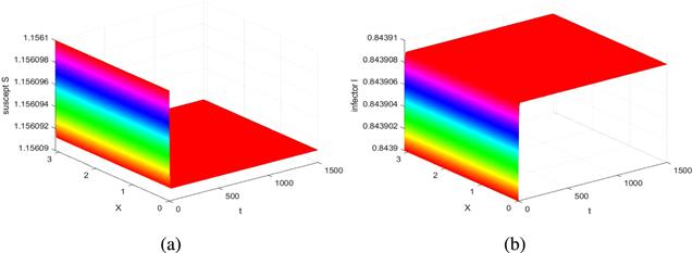
Figure 1. The equilibrium point E2 is locally asymptotically stable.

6.2. Case 2: I > Ic

When I > Ic, we need to verify the dynamic characteristics of the right-semi system. First, we take the parameter of the system (5) with A = 0.5, r = 0.1, μ = 0.1, β = 0.4, c = 0.6, Ic = 0.4, then we obtain b2 = 0.0790 > 0, b3 = 0.0250 > 0, Δ2 = 0.0514 > 0, which satisfies the existence condition of E5. According to equation (11), we have three solutions, one of them is E5 = (0.8743, 1.0367). Next, we need to change the value of diffusion coefficients to prove the stability of equilibria. When we let d1 = 0.01, d2 = 0.03, we find A11(E5) = 0.7361 > 0 and γ = 3 > γ3 = 0.0004. According to theorem 5.2, E5 is locally asymptotically stable as shown in figure 2.
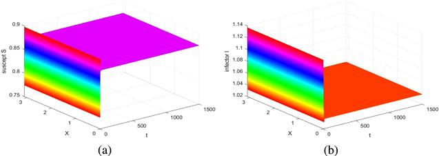
Figure 2. The equilibrium point E5 is locally asymptotically stable.
Moreover, we consider if the rumor spreading rate β changes, whether the positive equilibrium point will change. Fixing A = 0.5, r = 0.01, μ = 0.1, c = 0.55, Ic = 0.001, d1 = 0.01, d2 = 0.02 and only changing β from 0.3 to 0.7. Then as vividly shown in figure 3, we find as the rate of rumor spreading rate β increases, the number of people who spread rumors has also increased, and the stability of the component I for the equilibrium point E5 increases, which is in contradiction with the actual phenomenon.
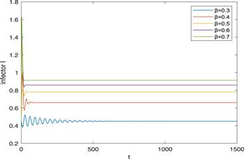
Figure 3. The influence of rumor propagation rate β on rumor spreaders.
Accordingly, we can study the instability of E5. Fixing A = 0.3, r = 0.001, μ = 0.05, β = 0.3, c = 0.8, Ic = 0.01, d1 = 0.01, d2 = 0.02. By simple calculation, we can find A11(E5) = − 0.0035 < 0, then the equilibrium point E5 = (0.2007, 2.7194) is unstable according to theorem 5.2, which is shown in figure 4.
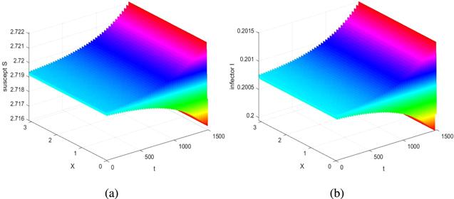
Figure 4. The equilibrium point E5 is unstable.
Next, we think about the Turing instability of E5 for system (5). Letting A = 0.5, r = 0.01, μ = 0.1, β = 0.3, c = 0.59, Ic = 0.01, d1 = 3.05, d2 = 0.1, then we have the equilibrium point E5 = (2.2460, 0.4013). We calculate A11(E5) = 0.0081 > 0, γ = 0.0328 < γ3 = 0.2040. Thus E5 is Turing unstable according to theorem 5.3. Observing the figure below, we can see when t = 100, the (figure 5(b)) is dominated by fuzzy bars. As time t gets bigger by 200, the main pattern of the figure is dotted bars. Then, the strips are separated into blue dots and stabilize in a stable form when t = 300. From figure 5(d), we can find three different values of S(x, t) as ${MAX}\left(S\right),{AVE}\left(S\right),{MIN}\left(S\right)$ stabilize at about 2.25 when t < 40, and then bifurcate from t = 40 and stabilize at a certain value around t = 180, respectively. Turing instability suggests that diffusion will cause an imbalance in the system, which is in line with the practical implications of rumor propagation; when the effects of catalysing rumor outbreaks are not aligned with curbing the spread of rumors, rumors will become uncontrollable.
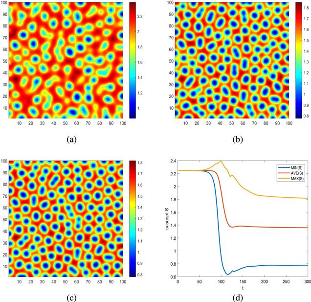
Figure 5. The Turing instability of E5.
Finally, we study the occurrence of Hopf bifurcation at E5 by changing the value of the parameter c. Taking A = 0.5, r = 0.01, μ = 0.1, β = 0.3, Ic = 0.001, d1 = 0.01, d2 = 0.02 at the same time, changing c from 0.5 to 0.9, then we find the stability of equilibrium point E5 switches. When c = 0.5, figure 6 shows that E5 is locally asymptotically stable, while c changes to 0.6, E5 becomes unstable, and it stabilizes again when c = 0.8.
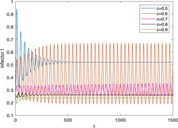
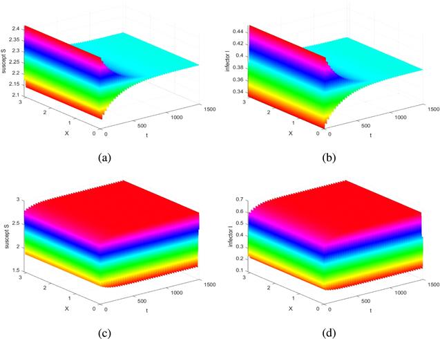
Figure 6. The change of stabilities for the equilibrium point E5.
We now study a concrete example. Taking A = 0.5, r = 0.01, μ = 0.1, β = 0.3, c = 0.6, Ic = 0.01, d1 = 0.01, d2 = 0.02, then we obtain E5 = (2.2764, 0.3915), A11(E5) =0.0082 > 0, and γ = 2 > γ3 = 0.1986. According to theorem 5.2, E5 is locally asymptotically stable, which is shown in figure 7(a) and (b). Then change the value of parameter Ic = 0.001, we have E5 = (2.3478, 0.3695), A11(E5) =−0.0097 < 0, from theorem 5.2, we know E5 is unstable, which is shown in figure 7(c) and (d). In short, Hopf bifurcation will occur at E5 when Ic changes from 0.001 to 0.01.
Figure 7. The Hopf bifurcation at E5.

7. Conclusion

In this article, we observe the actual relationship between I and the threshold Ic to establish a non-smooth rumor spreading model based on the time and space dimensions. Contrary to the smooth rumor propagation model of time delay, the non-smooth system is obviously a new addition to rumor propagation model collection. First of all, we prove the existence and uniqueness of the solution for system (5) according to the existence theorem of solutions. Secondly, we divide the system into two parts according to H(I, Ic) function and discuss the existence of the equilibrium points. For the left half of system (5), we define R0 to study the relationship between R0 and equilibrium points. Then we find that there is always an equilibrium point for the left half of the system. For the right half of system (5), we classify many different cases by discussing the coefficients of the equilibrium point equation. Then, on this basis, we perform a bifurcation analysis for the non-spatial system (12) and find conditions that make saddle-knot bifurcation exist. Further, we consider the effect of diffusion. According to the size relationship between I and Ic, we make specifically analyze the stability of equilibrium points for spatial system (5). In addition, we analyze the Turing instability and Hopf bifurcation occurring at equilibrium point E5. According to Lyapunov number, we determine the direction of the bifurcation. When I = Ic, we analyze and discuss conditions for the existence of discontinuous Hopf bifurcation. Finally, through numerical simulations and combined with the practical meaning of the parameters, we proved the correctness of the previous theoretical theorem.
In real life, rumor propagation is influenced by rumor control means and rumor propagation channels, and the non-smooth rumor propagation system can reflect this characteristic of rumor propagation. In addition, rumor propagation will change with time and the scope of rumor propagation. Therefore, the PDE model has more practical significance [2426].

Acknowledgments

This research is partly supported by the National Natural Science Foundation of China (Grant No. 12002135), China Postdoctoral Science Foundation (Grand No. 2023M731382), and the Young Science and Technology Talents Lifting Project of Jiangsu Association for Science and Technology.

Declaration of Competing Interest

The authors declare that they have no known competing financial interests or personal relationships that could have appeared to influence the work reported in this paper.
1
Daley D J Kendall D G 1964 Epidemics and rumours Nature 204 1118

DOI

2
Daley D J Kendall D G 1965 Stochastic rumours IMA J. Appl. Math. 1 42 55

DOI

3
Saikh A Gazi N H 2021 The effect of the force of infection and treatment on the disease dynamics of an SIS epidemic model with immigrants Res. Control Optim. 2 100007

DOI

4
Zhu L H Guan G Li Y 2019 Nonlinear dynamical analysis and control strategies of a network-based SIS epidemic model with time delay Appl. Math. Modell. 70 512 531

DOI

5
Fibich G 2016 Bass-SIR model for diffusion of new products in social networks Phys. Rev. E 94 032305

DOI

6
Sudbury A 1985 The proportion of the population never hearing a rumor J. Appl. Probab. 22 443 446

DOI

7
Qiu L 2021 SIR-IM:SIR rumor spreading model with influence mechanism in social networks Soft Computing 25 13949 13958

DOI

8
Zheng Z Y 2018 Factors influencing message dissemination through social media Phys. Rev. E 97 062306

DOI

9
Zan Y 2018 DSIR Double-rumors spreading model in complex networks Chaos Soliton Fractal 110 191 202

DOI

10
Xia L Jiang G Song B Song Y 2015 Rumor spreading model considering hesitating mechanism in complex social networks Physica A 437 295 303

DOI

11
Huo L Wang L Song G 2017 Global stability of a two-mediums rumor spreading model with media coverage Physica A 482 757 771

DOI

12
Zhao L 2013 A rumor spreading model with variable forgetting rate Physica A 392 6146 6154

DOI

13
Iannelli F Mariani M S Sokolov I M 2018 Influencers identification in complex networks through reaction-diffusion dynamics Phys. Rev. E 98 062302

DOI

14
Korosoglou P Kittas A Argyrakis P 2010 Spreading of infection in a two species reaction-diffusion process in networks Phys. Rev. E 82 061122

DOI

15
Trpevski D Tang W Kocarev L 2010 Model for rumor spreading over networks Phys. Rev. E 81 056102

DOI

16
Moreno Y Nekovee M Pacheco A F 2004 Dynamics of rumor spreading in complex networks Phys. Rev. E 69 066130

DOI

17
Liu X D Tao L Mi T 2018 Rumor spreading of a SEIR model in complex social networks with hesitating mechanism Adv. Differen. Equ. 1 391 415

18
Liu Q Li T Sun M 2017 The analysis of an SEIR rumor propagation model on heterogeneous network Physica A 469 372 380

DOI

19
Chen S 2020 Dynamical behaviors and optimal control of rumor propagation model with saturation incidence on heterogeneous networks Chaos Solitons Fractals 140 110206

DOI

20
Zhang T Teng Z 2008 Global asymptotic stability of a delayed SEIRS epidemic model with saturation incidence Chaos Solitons Fractals 37 1456 1468

DOI

21
Li C R Ma Z J 2015 Dynamic analysis of a spatial diffusion rumor propagation model with delay Adv. Differen. Equ. 1 364

22
Shi L Zhao H Y Wu D Y 2021 Dynamical analysis for a reaction–diffusion HFMD model with nonsmooth saturation treatment function Commun. Nonlinear Sci. Numer. Simul. 95 105593

DOI

23
Perko L 2001 Differential Equations and Dynamical Systems Berlin Springer

24
Ke Y 2022 Dynamics of a reaction–diffusion rumor propagation model with non-smooth control Appl. Math. Comput. 437 127478

25
Yuan T Y 2023 Stability analysis and optimal control of epidemic-like transmission model with nonlinear inhibition mechanism and time delay in both homogeneous and heterogeneous networks J. Math. Anal. Appl. 526 127273

DOI

26
Shi L 2022 Dynamics of an infection-age HIV diffusive model with latent infected cell and Beddington–DeAngelis infection incidence Eur. Phys. J. Plus 137 212

27
Zhu L H 2020 Global stability and bifurcation analysis of a rumor model with two discrete delays in social networks IJBC 30 2050175

DOI

28
Kuznetsov 2004 Elements of Applied Bifurcation Theory New York Springer

29
Ye Q X Li Z Y 1990 Introduction to Reaction–Diffusion Equation Beijing Science Press

Outlines

/