


1. Introduction
Partial differential equations (PDEs) are important tools for studying the laws of nature [1]. A large number of natural science and engineering problems can be described by differential equations, such as the motion of galaxies in the Universe, weather forecasting about temperature and wind speed, and the interaction between atoms [2, 3]. So far, PDEs have become an important link between mathematical theory and studies in the field of physics. There is no doubt that the development of the theory of PDEs has greatly advanced modern science and revolutionized many fields such as aerospace, radio wave communication, ocean exploration, and numerical weather prediction. However, solving most PDEs is very difficult, such as Maxwell’s equations in the field of electromagnetism and Navier–Stokes equations (NS) in the field of fluids. Due to their complexity and nonlinearity, it is difficult to find analytical solutions. Therefore, various numerical methods have been proposed to approximate the solutions of PDEs, such as finite difference method (FDM), finite element method (FEM), finite volume method (FVM), etc [4–7]. Although these methods have been widely used, they still have problems such as instability, error accumulation, and local truncation error. In addition to the problem of computational accuracy, the traditional numerical methods also have the problems of long computational time, high computational cost, and difficulty of grid dissection.
In recent years, deep learning technology has triggered a new wave of artificial intelligence research [8–10]. At present, deep learning has achieved great success in many fields such as image classification, natural language processing, and object detection [11, 12]. In addition to traditional research fields, the integration of artificial intelligence and natural sciences has received more and more attention [13–15]. At present, there have been many exciting research results in this cross-research field. For example, AlphaFold2 addresses the prediction of protein folding and three-dimensional structure [16]. Another hot work in this field is the application of deep neural networks to solve PDEs [17–19]. The theoretical basis of this research is the universal approximation theorem [20], that is, a multi-layer feedforward network with a sufficient number of hidden layer neurons can adequately approximate any continuous function. Mathematically, deep learning provides a tool for approximating high-dimensional functions. Traditional numerical methods often suffer from the curse of dimensionality, and deep neural networks can cope with this problem [21, 22]. Because for neural networks, the amount of computation brought about by the increase in dimension increases linearly. At the same time, compared to traditional grid-based methods such as the finite difference method and finite volume method, deep learning is a flexible, gridless method that is simpler to implement. In addition, in terms of hardware, it is easier for deep neural networks to take advantage of the hardware advantages of a graphics processing unit (GPU), thereby improving the speed of solving PDEs. Relevant researchers have carried out a lot of research, and the results show that neural network has unique advantages in the research of solving PDE [23–26]. Some researchers use neural networks instead of traditional numerical discretization methods to approximate the solutions of PDEs, for example, Lagaris et al used neural networks to solve the initial and boundary value problems [27, 28]. There are also some researchers who use neural networks to improve the traditional numerical solutions of PDEs, thereby improving the computational efficiency of existing methods [29, 30]. Among many works, one of the most representative achievements is the related work of physics-informed neural networks (PINNs) [31–35], which proposes a new composite loss function. The loss function consists of four parts: observation data constraints, PDE constraints, boundary condition constraints, and initial condition constraints. PINNs encode physics governing equations into neural networks, significantly improving the performance of neural network models. In terms of programming implementation, PINNs take full advantage of the automatic differentiation framework [36]. Currently, automatic differentiation mechanisms are widely used in deep learning frameworks. Different from symbolic differentiation and numerical differentiation, automatic differentiation relies on the concept of computational graph, performs symbolic differentiation within each computational graph node, and uses numerical values to store the differential results between nodes. Therefore, the automatic differentiation mechanism is more accurate than numerical differentiation and more efficient than symbolic differentiation. After PINNs was proposed, a large number of researchers have studied and improved the original PINNs, proposed various improved PINNs and applied them in many fields, showing great application prospects [37–41]. Chen et al have carried out a large number of simulation studies on localized wave solutions of the integrable equations using deep learning methods, which can effectively characterize their dynamical behaviors, and proposed the theoretical architecture and development direction of integrable deep learning, which has promoted the related research on nonlinear mathematical physics and integrable systems [42–47]. In recent years, with the rapid development of ocean sound field calculation, atmospheric pollution diffusion simulation, seismic wave inversion and prediction, etc [48–50], higher requirements are put forward for the accuracy and efficiency of numerical methods, and it is urgent to develop new methods and tools for solving PDE. The researchers have used physics-informed neural networks to solve the frequency-domain wave equation, simulated seismic multifrequency wavefields, and conducted in-depth research on wave propagation and full waveform inversions, and achieved a series of research results [51–55]. It is expected that PINNs can provide a new opportunity to solve a large number of scientific and engineering problems at the present time, and bring breakthroughs in the relevant research.
Aiming at the problem of solitary wave solutions in the research of PDEs, this study uses improved PINNs to carry out solitary wave simulation research. Compared with the original PINNs, the improved PINNs modified the activation function in the neural network. Specifically, hyperparameters are introduced into the activation function to change the slope of the activation function and avoid the disappearance of the gradient, thereby saving computing time and speeding up training. The structure of this paper is as follows. Section 2 introduces PINNs with adaptive activation functions. Next, section 3 gives the specific mathematical forms and experimental schemes of the mKdV equation, the improved Boussinesq equation, the Caudrey–Dodd–Gibbon–Sawada–Kotera (CDGSK) equation and the p-gBKP equation, and then constructs the corresponding neural network to carry out numerical experiments and analyzes the experimental results. Finally, section 4 summarizes our work and and look forward to future research directions.
2. Method
This section focuses on how to improve PINNs with adaptive mechanisms for solving PDEs with solitary wave solutions. The basic idea of PINNs is to introduce the control equation as a regularization term into the loss function of the neural network, so as to transform the problem of solving PDEs in physical space into the optimization problem of neural network parameters, and then obtain the approximation solution of PDEs by training the neural network. Next, PINNs and adaptive mechanisms will be introduced in detail.
2.1. Physics-informed neural networks
From the perspective of mathematical function approximation theory, a neural network can be regarded as a general nonlinear function approximator. On the other hand, the problem of solving PDEs is to find nonlinear functions that satisfy constraints. Therefore, there is a certain connection between neural networks and PDEs. Raissi et al [31] used limited observation data and control equations, as well as initial and boundary conditions to construct residual terms, and used the sum of them to construct a loss function, and proposed PINNs under physical constraints. The neural network trained in this way can not only approximate the observation data, but also automatically satisfy the symmetry, invariance, conservation and other physical properties followed by PDEs. The design idea of PINNs is to combine data-driven with physical constraints, which provides a new idea for solving PDEs. For the following PDE:
$\begin{eqnarray}\begin{array}{rcl}{u}_{t}+{{ \mathcal N }}_{x}[u] & = & 0,\quad x\in {\rm{\Omega }},t\in [{T}_{0},T]\\ u(x,{T}_{0}) & = & h(x),\quad x\in {\rm{\Omega }}\\ u(x,t) & = & g(x,t),\quad x\in \partial {\rm{\Omega }},t\in [{T}_{0},T].\end{array}\end{eqnarray}$
In the above formula, t and x represent the time variable and space variable respectively, T and Ω represent their value ranges respectively, and ∂Ω is the boundary of the space domain Ω. ${{ \mathcal N }}_{x}$ is a combination of linear and nonlinear operators, h(x) is the initial condition, and g(x, t) is the boundary condition.To get the approximate solution of PDE, we first construct a neural network $\widehat{u}(x,t;\theta )$, where θ represents the parameters of the neural network. The neural network $\widehat{u}(x,t;\theta )$ should meet two requirements: on the one hand, the neural network is first trained using the observed data set, and later, when tested, the trained model should be able to output accurate function values for the input variables; on the other hand, it should conform to the physical constraints of PDEs. Here, the automatic differential technique is used to integrate the differential constraints in the PDE into the neural network, and a residual network is constructed to meet the requirements of the second term. Mathematically, the definition of a residual network is shown in formula (2).
$\begin{eqnarray}f(x,t;\theta ):= \displaystyle \frac{\partial }{\partial t}\widehat{u}(x,t;\theta )+{{ \mathcal N }}_{x}[\widehat{u}(x,t;\theta )].\end{eqnarray}$
The next task is to construct the loss function of PINNs, which mainly consists of four parts, including observation data constraints, governing equation constraints, initial condition constraints and boundary condition constraints. Mathematically, the four parts are defined as follows.3 ) represents the loss term calculated according to the observation data, and the quality of the observation data will directly affect the effectiveness of the training. Equation (4 ) represents the PDE residual term calculated based on the selected residual points. All residual points are randomly selected in the time and space domains, and Nf is the number of selected residual points. Equation (4 ) requires the neural network to satisfy the constraints of PDEs, which are also known as physical information regularization terms. Equation (5 ) represents the loss term calculated from the initial condition, which requires the neural network to satisfy the constraints of the initial condition. Equation (6 ) represents the loss term calculated according to the boundary conditions, which requires the neural network to satisfy the constraints of the boundary conditions. Finally, the mathematical expression of the loss function to be optimized is as follows
$\begin{eqnarray}{L}_{{\rm{o}}}\left(\theta ;{N}_{{\rm{o}}}\right)=\displaystyle \frac{1}{2\left|{N}_{{\rm{o}}}\right|}\displaystyle \sum _{j=1}^{{N}_{{\rm{o}}}}{\parallel \hat{u}\left({x}_{{\rm{o}}}^{j},{t}_{{\rm{o}}}^{j};\theta \right)-{u}_{{\rm{o}}}^{j}\parallel }_{2}^{2}\end{eqnarray}$
$\begin{eqnarray}{L}_{\mathrm{PDE}}\left(\theta ;{N}_{f}\right)=\frac{1}{2\left|{N}_{f}\right|}\displaystyle \sum _{j=1}^{{N}_{f}}{\parallel f\left({x}_{f}^{j},{t}_{f}^{j};\theta \right)\parallel }^{2}\end{eqnarray}$
$\begin{eqnarray}{L}_{\mathrm{IC}}\left(\theta ;{N}_{i}\right)=\frac{1}{2\left|{N}_{i}\right|}\displaystyle \sum _{j=1}^{{N}_{i}}{\parallel \hat{u}\left({x}_{i}^{j},0;\theta \right)-{h}_{i}^{j}\parallel }_{2}^{2}\end{eqnarray}$
$\begin{eqnarray}{L}_{\mathrm{BC}}\left(\theta ;{N}_{b}\right)=\frac{1}{2\left|{N}_{b}\right|}\displaystyle \sum _{j=1}^{{N}_{b}}{\parallel \hat{u}\left({x}_{b}^{j},{t}_{b}^{j};\theta \right)-{g}_{b}^{j}\parallel }_{2}^{2}.\end{eqnarray}$
Equation ( $\begin{eqnarray}\begin{array}{rcl}L(\theta ;N) & = & {\lambda }_{o}{L}_{o}\left(\theta ;{N}_{o}\right)+{\lambda }_{f}{L}_{{PDE}}\left(\theta ;{N}_{f}\right)\\ & & +{\lambda }_{b}{L}_{{BC}}\left(\theta ;{N}_{b}\right)+{\lambda }_{i}{L}_{{IC}}\left(\theta ;{N}_{i}\right),\end{array}\end{eqnarray}$
where λ = {λo, λf, λb, λi} is a vector of weight coefficients of the loss function. The weight coefficient of each loss item in this study is set to 1.0. Next, gradient descent methods, such as Adam, Stochastic Gradient Descent (SGD) or L-BFGS, are used to find the minimum value of the loss function. By continuously optimizing the parameters of the neural network, the value of the loss function decreases, so that the output of the neural network is close to the true solution of the PDE. The framework of the physics-informed neural networks is shown in figure 1.
Figure 1. Schematic of physics-informed neural networks for solving partial differential equation. |
2.2. The improved physics-informed neural networks with adaptive activation function
The activation function is an important component of artificial neural networks and governs the behavior of neurons, such as whether to process the input data and how to process it. In a specific implementation, the activation function of a particular node processes the input information of the previous node in the neural network and outputs a deterministic value which then guides the subsequent nodes on how to respond to a particular input signal. The main purpose of using the activation function in the neural network model is to introduce nonlinear characteristics into the neural network and strengthen the learning ability of the neural networks, so that it can learn complex physical systems. Without the nonlinear activation function, a neural network with many hidden layers will become a giant linear regression model, which is useless for learning complex mathematical models from observation data. Studies have shown that using different types of activation functions in the neural network, the performance of the neural network model will show a large difference. Therefore, when building a neural network model, it is a critical task to select the appropriate activation function according to the actual problem to be solved. Currently, researchers have proposed many kinds of activation functions for building neural network models. For example, the Sigmoid function is a widely used activation function, which outputs a function value in the range (0, 1) for any input value. Very similar to the Sigmoid function is the tanh function, whose output value ranges from (−1, 1). Unlike the Sigmoid function and the tanh function, the ReLU function is a piecewise function. When its input value is less than zero, its output value is zero. When its input value is greater than zero, the ReLU function is the function y = x. In addition to the above activation functions, widely used activation functions include the leaky ReLU function, Maxout function, ELU function, Parametric ReLU function, and so on.
In order to improve the original PINNs to achieve better performance in solving PDEs, Jagtap et al modified the activation function in PINNs to an adaptive activation function [56, 57], thus speeding up the training convergence. The specific method is to introduce a hyperparameter a into the activation function and optimize this parameter as a neural network parameter. When training a neural network, the slope of the activation function changes as the hyperparameter a changes. Studies have shown that adaptive activation functions have better learning ability than traditional activation functions, and can improve the convergence speed of neural networks in early training. Here, taking several classical activation functions as examples, their mathematical formulas are modified into the following form
$\begin{eqnarray}\mathrm{Sigmoid}(x)=\frac{1}{1+{{\rm{e}}}^{-{ax}}}\end{eqnarray}$
$\begin{eqnarray}\tanh (x)=\frac{{{\rm{e}}}^{{ax}}-{{\rm{e}}}^{-{ax}}}{{{\rm{e}}}^{{ax}}+{{\rm{e}}}^{-{ax}}}\end{eqnarray}$
$\begin{eqnarray}\mathrm{ReLU}(x)=\max (0,{ax})\end{eqnarray}$
$\begin{eqnarray}\mathrm{Leaky}\ \mathrm{ReLU}(x)=\max (0,{ax})-v\max (0,-{ax}).\end{eqnarray}$
Aiming at the solitary wave simulation problem in this study, considering that solitary waves are a kind of localized traveling waves when constructing the neural network, we chose the Neuron-wise locally adaptive activation functions (N-LAAF), which are defined as follows:
$\begin{eqnarray}\begin{array}{l}\sigma \left({{na}}_{i}^{l}{\left({{ \mathcal L }}_{l}\left({z}^{l-1}\right)\right)}_{i}\right),\quad l=1,2,\ldots ,M-1,\\ \,i=1,2,\ldots ,{N}_{k}\end{array}\end{eqnarray}$
where n ≥ 1 is an inflation factor, M is the number of layers of the neural network, and Nk is the number of neurons. At this point, the objects to be optimized include not only weights and biases but also activation slopes. With the introduction of the N-LAAF, the solution obtained based on the improved PINN is as follows: $\begin{eqnarray}\begin{array}{l}{u}_{\hat{{\boldsymbol{\Theta }}}}(x)=({{ \mathcal L }}_{M}\circ \sigma \circ {{na}}_{i}^{M-1}{\left({{ \mathcal L }}_{M-1}\right)}_{i}\circ \cdots \\ \quad \circ \sigma \circ {{na}}_{i}^{1}..\times {\left({{ \mathcal L }}_{1}\right)}_{i})(x).\end{array}\end{eqnarray}$
To further avoid gradient disappearance, the adaptive activation function defines a slope recovery term Laaf(a) to increase the slope of the activation function:
$\begin{eqnarray}{L}_{{aaf}}(a)=\displaystyle \frac{1}{\tfrac{1}{M-1}{\sum }_{k=1}^{M-1}\exp \left({\left(\tfrac{{\sum }_{i=1}^{{N}_{k}}{a}_{i}^{k}}{{N}_{k}}\right)}^{2}\right)}.\end{eqnarray}$
By analyzing the above formula, it is found that with the increase of the slope of the activation function, the value of this term decreases. Therefore, this item is added to the loss function and optimized by optimization method. At this point, the new loss function is defined as follows:
$\begin{eqnarray}\begin{array}{l}L(\hat{{\boldsymbol{\Theta }}};N)={\lambda }_{o}{L}_{o}\left(\hat{{\boldsymbol{\Theta }}};{N}_{o}\right)+{\lambda }_{f}{L}_{\mathrm{PDE}}\left(\hat{{\boldsymbol{\Theta }}};{N}_{f}\right)\\ \quad +\,{\lambda }_{b}{L}_{\mathrm{BC}}\left(\hat{{\boldsymbol{\Theta }}};{N}_{b}\right)+{\lambda }_{i}{L}_{{IC}}\left(\hat{{\boldsymbol{\Theta }}};{N}_{i}\right)\\ \quad +\,{\lambda }_{a}{L}_{{aaf}}(a).\end{array}\end{eqnarray}$
Next, similar to the training process of the original PINNs, we use the optimization algorithm to update the parameters of the improved PINNs so that the loss function value keeps decreasing. Eventually, the output of the neural network will gradually close to the exact solution of the nonlinear soliton equations.
3. Numerical experiments and results
In this section, we have simulated solitary wave solutions of several PDEs using the above method. Solitary waves play an important role in the field of nonlinear science and their theory is applied in many fields such as fluid mechanics, quantum mechanics, nonlinear fibre optic communication, etc. Therefore, the problem of solitary wave simulation has received a lot of attention from researchers. In this section, we use the improved PINNs to approximate the soliton solutions of the mKdV equation [58], the improved Boussinesq equation [59], the CDGSK equation [60], and the p-gBKP equation. In addition, we analyze the convergence speed and accuracy of the proposed method. The accuracy of the approximate solution of the neural network is measured by the relative L2 error
$\begin{eqnarray}{\rm{L}}2\ \mathrm{error}=\displaystyle \frac{\sqrt{{\sum }_{i=1}^{N}{\left|\hat{u}\left({x}_{i},{t}_{i}\right)-u\left({x}_{i},{t}_{i}\right)\right|}^{2}}}{\sqrt{{\sum }_{i=1}^{N}{\left|u\left({x}_{i},{t}_{i}\right)\right|}^{2}}}.,\end{eqnarray}$
where $u\left({x}_{i},{t}_{i}\right)$ represents the exact solution and $\hat{u}\left({x}_{i},{t}_{i}\right)$ represents the approximate solution.3.1. The numerical solution for the modified Korteweg–de Vries (mKdV) equation
The mKdV equation can be used as a model to describe acoustic waves in anharmonic lattices, and can also be used to study solitary waves in nonlinear optics. In this section, the solitary wave solution of the mKdV equation is studied. The mathematical form of the mKdV equation is as follows:
$\begin{eqnarray}{u}_{t}+6{u}^{2}{u}_{x}+{u}_{{xxx}}=0.\end{eqnarray}$
3.1.1. The single soliton solution of mKdV equation
Given the following initial conditions:
$\begin{eqnarray}u(x,0)={\rm{{\rm{sech}} }}(x-{x}_{0}).\end{eqnarray}$
In this problem, the value of x0 is 0, and the spatial domain is in the range [−8, 8]. In terms of time, T = 5, that is, the simulation duration is 5. The true solution to the equation is as follows:
$\begin{eqnarray}\begin{array}{l}u(x,t)={\rm{sech}} (x-t-{x}_{0}),\quad x\in [-8,8],\\ t\in [0,5].\end{array}\end{eqnarray}$
Next, we construct a neural network, which contains 4 hidden layers, the number of neurons in the hidden layer is 32, and the activation function is the adaptive activation function. During training, the supervised data is randomly drawn from the true data. In this study, the initial condition is regarded as a special type of Dirichlet boundary condition in the space-time domain. During the training process, the data regarding initial and boundary conditions were obtained by random sampling, and the number of samples was 300. In order to construct physical constraints, the residual points are randomly selected in the space-time domain, and the amount of data sampled in this experiment is 10 000. In addition, we use a small number of observations, the number of observations in this experiment is 200. In the optimization process, in order to balance the convergence speed and global convergence, L-BFGS is used to complete 5000 epoch iterations, and then Adam is used to continue the optimization until convergence. The learning rate is set to 0.001 during training. After training, the trained model is used to approximate the solution of the PDE. Figure 2 shows the true solution of the mKdV equation in this section and the predicted results obtained using the trained model. It can be seen from figure 2 that the two are highly consistent, and the neural network model simulates the characteristics of a single soliton. In order to further analyze the experimental results intuitively, the prediction results at different times are selected for comparison with the exact solution to test the accuracy of the prediction results. Figure 3 shows a comparison of the true and approximate solutions of the PDE at different times, and it can be seen that the predicted values are very close to the true solution. In addition, the error between the approximate solution of the neural network and the true solution is counted through many experiments, and the relative L2 norm error between the predicted result and the true solution is about 1.73 × 10⁻³. Under the same training data and parameter settings, the relative L2 norm error between the prediction results calculated by the original PINNs and the true solution is about 2.78 × 10⁻³. Figure 4 shows the error statistics of the improved PINNs and the original PINNs. Finally, the training time was analysed and it was found that the average time to complete the training task for the improved PINNs was approximately 58.5% of the training time for the original PINNs. Experiments demonstrate that the improved PINNs outperform the original PINNs in both training efficiency and accuracy for single solitary wave simulation problems of the mKdV equation.

Figure 2. The exact single soliton solution (top) and learned solution (bottom) of the mKdV equation. |
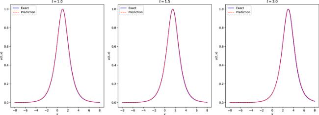
Figure 3. Comparison of the exact single soliton solution of the mKdV equation and the approximate solution of the neural network at different moments. |
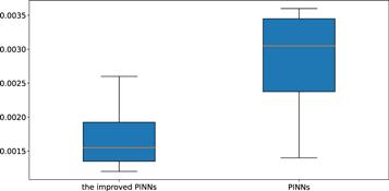
Figure 4. Error statistics for the improved PINNs and the original PINNs for solving single-soliton solutions of the mKdV equation. |
3.1.2. The double soliton solution of mKdV equation
Next, we further study the double-soliton solution of the mKdV equation, given the following initial conditions:
$\begin{eqnarray}u(x,0)={\rm{{\rm{sech}} }}(x+4)+{\rm{{\rm{sech}} }}(x-4).\end{eqnarray}$
In this problem, the spatial domain is in the range [−10, 10]. In terms of time, T = 10, that is, the simulation duration is 10. The true solution of the mKdV equation is as follows:
$\begin{eqnarray}u(x,t)={\rm{{\rm{sech}} }}(x-t+4)+{\rm{{\rm{sech}} }}(x-t-4).\end{eqnarray}$
Next, similar to the single-soliton simulation problem, we first construct a neural network with 5 hidden layers and 32 neurons in each hidden layer, and the activation function is set to the adaptive activation function. During training, the initial condition is also treated as a special type of Dirichlet boundary condition in the space-time domain. The data regarding initial and boundary condition were obtained by random sampling, and the number of samples was 400. In order to construct physical constraints, the residual points are randomly selected in the space-time domain, and the amount of data sampled in this experiment is 15 000. Meanwhile, we use a small number of observations, the number of observations in this experiment is 300. In the optimization process, in order to balance the convergence speed and global convergence, L-BFGS is also used to complete 5000 epoch iterations, and then Adam is used to continue the optimization until convergence. The learning rate is set to 0.001 during training. After training, the trained model is used to approximate the double-soliton solution of the mKdV equation. Figure 5 shows the exact solution and the predicted results using the trained model. It can be seen from the figure that the two are highly consistent, and the neural network model simulates the characteristics of the double soliton. Similarly, in order to further analyze the experimental results intuitively, the prediction results at different times are selected to be compared with the exact solution to check the accuracy of the prediction results. Figure 6 shows the comparison of the true and approximate solutions of the mKdV equation at different times, and it can be seen that the predicted values are very close to the true solutions. In addition, the error between the approximate solution and the exact solution of the neural network is counted through many experiments, and the relative L2 norm error between the predicted result and the exact solution is about 1.94 × 10⁻³. Under the same training data and parameter settings, the relative L2 norm error between the prediction results calculated by the original PINNs and the exact solution is about 3.32 × 10⁻³. Figure 7 shows the error statistics of the improved PINNs and the original PINNs. Finally, the training time was analysed and it was found that the average time to complete the training task for the improved PINNs was approximately 61.3% of the training time for the original PINNs. Experiments show that for the double soliton simulation problem, the improved PINNs are superior to the original PINNs in both training efficiency and accuracy.
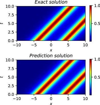
Figure 5. The exact two soliton solutions (top) and learned solution(bottom) of the mKdV equation. |
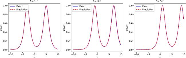
Figure 6. Comparison of the exact double soliton solution of the mKdV equation and the approximate solution of the neural network at different moments. |
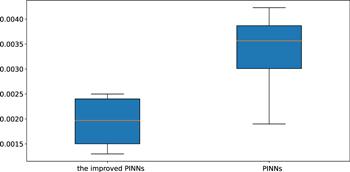
Figure 7. Error statistics for the improved PINNs and the original PINNs for solving two-soliton solutions of the mKdV equation. |
3.2. The numerical solution for the improved Boussinesq equation
In this section, the solitary wave solution of the improved Boussinesq equation is considered. The Boussinesq equation is a fairly effective mathematical model that can describe the refraction, diffraction and reflection effects of regular and irregular waves on complex terrain. With the development of computer technology, the Boussinesq equation has been popularized for deep-water short-wave research and has become a powerful tool for simulating wave motion in nearshore areas. The mathematical form of the classical Boussinesq equation is as follows:
$\begin{eqnarray}\begin{array}{l}{u}_{{tt}}={u}_{{xx}}+{{qu}}_{{xxxx}}+r{\left({u}^{2}\right)}_{{xx}},\quad x\in [{L}_{1},{L}_{2}],\\ t\in [{T}_{0},T].\end{array}\end{eqnarray}$
With the continuous development of related research, Bogolubsky proposed an improved Boussinesq (IBq.) equation [61]. The mathematical expression of the improved Boussinesq equation is as follows:
$\begin{eqnarray}\begin{array}{rcl}{u}_{{tt}} & = & {u}_{{xx}}+{u}_{{xxtt}}+{\left({u}^{2}\right)}_{{xx}},\\ u(x,0) & = & \phi (x),\quad \\ {u}_{t}(x,0) & = & \psi (x)\\ u(-L,t) & = & u(L,t).\end{array}\end{eqnarray}$
Next, examples with different initial conditions will be selected to analyze the effectiveness of the improved PINNs.
3.2.1. The single soliton solution of the improved Boussinesq equation
First, the initial conditions and boundary condition are given as follows:
$\begin{eqnarray}u(x,0)=A{{\rm{sech}} }^{2}\left(\displaystyle \frac{1}{c}\sqrt{\displaystyle \frac{A}{6}}x\right)\end{eqnarray}$
$\begin{eqnarray}{u}_{t}(x,0)=2A{{\rm{sech}} }^{2}\left(\displaystyle \frac{1}{c}\sqrt{\displaystyle \frac{A}{6}}x\right)\tanh \left(\displaystyle \frac{1}{c}\sqrt{\displaystyle \frac{A}{6}}x\right)\end{eqnarray}$
$\begin{eqnarray}u(-L,t)=u(L,t),\end{eqnarray}$
where A = 0.25 and c = $\sqrt{7/6}$. The range of the space-time domain is x ∈ [ −10, 10], t ∈ [0, 10]. The exact solution of the improved Boussinesq equation at this time is as follows: $\begin{eqnarray}u(x,t)=0.25{{\rm{sech}} }^{2}\left(\displaystyle \frac{1}{2\sqrt{7}}\left(x-\sqrt{7/6}t\right)\right).\end{eqnarray}$
Next, similar to solving the solution to the mKdV equation, we first construct a neural network with 5 hidden layers, where the number of neurons in the hidden layer is 32, and we choose the adaptive activation function to build the neural network. During training, the initial conditions are also treated as a special type of Dirichlet boundary conditions in the space-time domain. The data regarding initial and boundary condition were obtained by random sampling, and the number of samples was 400. Similarly, residual points are randomly selected in the space-time domain to construct physical constraints, and the amount of data sampled in this experiment is 20 000. In addition, we use a small number of observations, the number of observations in this experiment is 300. In order to improve the convergence speed and achieve global convergence, we first use L-BFGS to complete 5000 epoch iterations, and then use Adam to continue optimizing until convergence. The learning rate of this experiment is set to 0.001. After training, the trained model is used to approximate the single-soliton solution of the improved Boussinesq equation. Figure 8 shows the exact solution and the predictions obtained using the trained model. It can be seen from figure 8 that the two are very consistent, and the neural network model simulates the characteristics of the single soliton of the improved Boussinesq equation. Similarly, in order to further analyze the experimental results intuitively, the prediction results at different times are selected to be compared with the exact solution to check the accuracy of the prediction results. Figure 9 shows a comparison of the true and approximate solutions of the improved Boussinesq equation at different times. It can be seen that the predicted values are very close to the exact solution. In addition, through many experiments, the error between the approximate solution and the exact solution is counted, and the relative L2 norm error between the predicted result and the exact solution is about 2.13 × 10⁻³. Under the same training data and parameter settings, the relative L2 norm error between the prediction results calculated by the original PINNs and the true solution is about 2.91 × 10⁻³. Figure 10 shows the error statistics of the improved PINNs and the original PINNs. Finally, the training time was analysed and it was found that the average time to complete the training task for the improved PINNs was approximately 63.3% of the training time for the original PINNs. Experiments show that for the single soliton simulation problem of the improved Boussinesq equation, the improved PINNs are superior to the original PINNs in both training efficiency and accuracy.
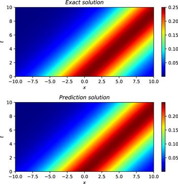
Figure 8. The exact single soliton solution (top) and learned solution (bottom) of the improved Boussinesq equation. |
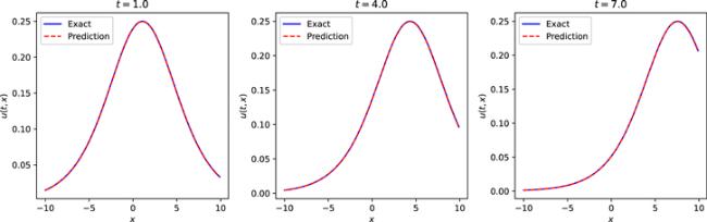
Figure 9. Comparison of the exact single soliton solution of the improved Boussinesq equation and the approximate solution of the neural network at different moments. |
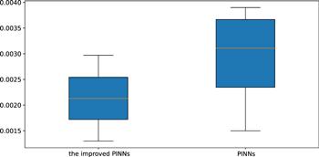
Figure 10. Error statistics for the improved PINNs and the original PINNs for solving single soliton solutions of the improved Boussinesq equation. |
3.2.2. The double soliton solution of the improved Boussinesq equation
Next, we further investigate the double-soliton solution of the improved Boussinesq equation, given the following initial conditions:
$\begin{eqnarray}u(x,0)=\displaystyle \sum _{i=1}^{2}{A}_{i}{{\rm{sech}} }^{2}\left(\displaystyle \frac{1}{{c}_{i}}\sqrt{\displaystyle \frac{{A}_{i}}{6}}\left(x-{x}_{0}^{i}\right)\right),\end{eqnarray}$
$\begin{eqnarray}\begin{array}{rcl}{u}_{t}(x,0) & = & 2\displaystyle \sum _{i=1}^{2}{A}_{i}{{\rm{sech}} }^{2}\left(\displaystyle \frac{1}{{c}_{i}}\sqrt{\displaystyle \frac{{A}_{i}}{6}}\left(x-{x}_{0}^{i}\right)\right)\\ & & \times \,\tanh \left(\displaystyle \frac{1}{{c}_{i}}\sqrt{\displaystyle \frac{{A}_{i}}{6}}\left(x-{x}_{0}^{i}\right)\right),\end{array}\end{eqnarray}$
$\begin{eqnarray}u(-L,t)=u(L,t).\end{eqnarray}$
In the above equation, A1 = A2 = 1.5, ${x}_{0}^{1}=-4$, ${x}_{0}^{2}=4$, ${c}_{1}=\sqrt{\tfrac{2{A}_{1}}{3}+1}$, ${c}_{2}=-\sqrt{\tfrac{2{A}_{2}}{3}+1}$. In this problem, L = 10, i.e. the spatial domain range is [−10, 10]. In the time domain, T = 6, i.e. the simulation time is 6.
Next, we build a neural network with 5 hidden layers, where the number of neurons in the hidden layer is 32, and the activation function is still the adaptive activation function. The initial conditions are still considered a special type of Dirichlet boundary conditions in the space-time domain. The data regarding initial and boundary conditions were obtained by random sampling, and the number of samples was 500. Residual points are randomly selected in the space-time domain to construct physical constraints. The number of residual points sampled in this experiment is 20,000. Meanwhile, we use a small number of observations, the number of observations in this experiment is 300. During training, we first use L-BFGS to complete 5000 epoch iterations, and then use Adam to continue optimizing until convergence. The learning rate of this experiment is set to 0.001. After training, we use the trained model to approximate the double-soliton solution of the improved Boussinesq equation. Figure 11 shows the exact solution and the predicted results using the trained model. As can be seen from the figure, the neural network successfully simulates the characteristics of the double-soliton of the improved Boussinesq equation. Similarly, in order to further analyze the experimental results intuitively, the prediction results at different times are selected to be compared with the exact solution to check the accuracy of the prediction results. Figure 12 shows a comparison of the true and approximate solutions of the improved Boussinesq equation at different times. It can be seen that the predicted values are very close to the true solution. In addition, through many experiments, the error between the approximate solution and the exact solution of the neural network is counted, and the relative L2 norm error between the predicted result and the exact solution is about 2.28 × 10⁻³. Under the same training data and parameter settings, the relative L2 norm error between the prediction results calculated by the original PINNs and the exact solution is about 3.19 × 10⁻³. Figure 13 shows the error statistics of the improved PINNs and the original PINNs. Finally, the training time was analysed and it was found that the average time to complete the training task for the improved PINNs was approximately 54.9% of the training time for the original PINNs. Experiments show that for the double-soliton simulation problem of the improved Boussinesq equation, the improved PINNs have certain advantages in both training efficiency and accuracy.
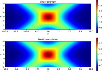
Figure 11. The exact double soliton solution (top) and learned solution (bottom) of the improved Boussinesq equation. |
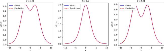
Figure 12. Comparison of the exact double soliton solution of the improved Boussinesq equation and the approximate solution of the neural network at different moments. |
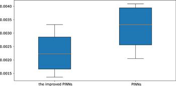
Figure 13. Error statistics for the improved PINNs and the original PINNs for solving two soliton solutions of the improved Boussinesq equation. |
3.3. The numerical solution for the CDGSK equation
In this section, the solitary waves solution of the CDGSK equation are studied. The mathematical form of the CDGSK equation is defined as follows:
$\begin{eqnarray}{u}_{t}+{u}_{{xxxxx}}+30{{uu}}_{{xxx}}+30{u}_{x}{u}_{{xx}}+180{u}^{2}{u}_{x}=0.\end{eqnarray}$
Next, the single and double soliton solutions of the CDGSK equation will be studied based on the improved PINNs.
3.3.1. The single soliton solution of CDGSK equation
The initial condition is given as follows:
$\begin{eqnarray}u(x,0)=\displaystyle \frac{{k}^{2}}{4}{{\rm{sech}} }^{2}\left(\displaystyle \frac{1}{2}{kx}+C\right).\end{eqnarray}$
In the above formula, the value of k is 0.8, the value of C is 0, the spatial range is [−7, 7], and the time range is [0, 6]. Under the above conditions, the single soliton solution of the CDGSK equation is given as follows: $\begin{eqnarray}u(x,t)=\displaystyle \frac{{k}^{2}}{4}{{\rm{sech}} }^{2}\left(\displaystyle \frac{1}{2}{kx}-\displaystyle \frac{1}{2}{k}^{5}t+C\right).\end{eqnarray}$
Next, we build a neural network with 7 hidden layers, where the number of neurons in the hidden layer is 32, and the activation function is still adaptive activation function. For the initial condition, it is still regarded as a special type of Dirichlet boundary condition in the space-time domain. The training data regarding the initial and boundary conditions were obtained by random sampling with a sample size of 500. Residual points are randomly selected in the space-time domain to construct physical constraints, and the amount of data sampled in this experiment is 15 000. In addition, we utilized a small number of observations, which numbered 400. During training, the learning rate is set to 0.001, and L-BFGS is used to complete 5000 epoch iterations, and then Adam is used to continue the optimization until convergence. Once training was complete, we employed the trained model to approximate the single-soliton solution of the CDGSK equation. Figure 14 shows the exact solution and the predicted results using the trained model. As can be seen from the figure, the neural network successfully simulates the single-soliton solution of the CDGSK equation. Similarly, in order to further analyze the experimental results intuitively, the prediction results at different times are selected to be compared with the exact solution to check the accuracy of the prediction results. Figure 15 shows the comparison of the true and approximate solutions of the single-soliton solution of the CDGSK equation at different times. It can be seen that the predicted value is very close to the true solution. In addition, the error between the approximate solution and the exact solution is counted through many experiments, and the relative L2 norm error between the predicted result and the exact solution is about 2.09 × 10⁻³. Under the same training data and parameter settings, the relative L2 norm error between the prediction results calculated by the original PINNs and the exact solution is about 2.84 × 10⁻³. Figure 16 shows the error statistics of the improved PINNs and the original PINNs. Finally, the training time was analysed again and it was found that the average time to complete the training task for the improved PINNs was approximately 61.7% of the training time for the original PINNs. Experiments show that the improved PINNs are more efficient in training than the original PINNs for the single-soliton solution simulation problem of the CDGSK equation.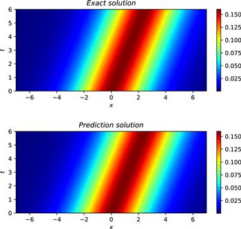
Figure 14. The exact single soliton solution (top) and learned solution (bottom) of the CDGSK equation. |
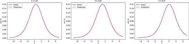
Figure 15. Comparison of the exact single soliton solution of the CDGSK equation and the approximate solution of the neural network at different times. |
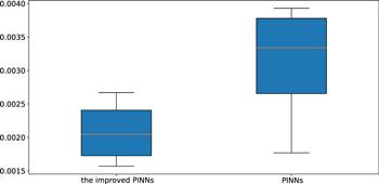
Figure 16. Error statistics for the improved PINNs and the original PINNs for solving single soliton solutions of the CDGSK equation. |
3.3.2. The two soliton solution of CDGSK equation
First, the initial condition is given as follows:
$\begin{eqnarray}u(x,0)=\displaystyle \frac{-4{dk}\mu \sinh \xi \sinh \eta +2d\left({k}^{2}+{\mu }^{2}\right)\cosh \xi \cosh \eta +{k}^{2}+4{d}^{2}{\mu }^{2}}{{\left(\cosh \xi +2d\cosh \eta \right)}^{2}},\end{eqnarray}$
$\begin{eqnarray}\xi ={kx},\end{eqnarray}$
$\begin{eqnarray}\eta =\mu x.\end{eqnarray}$
In the above formula, $d=\tfrac{k}{2\mu }\sqrt{\tfrac{3{k}^{2}+{\mu }^{2}}{{k}^{2}+3{\mu }^{2}}}$, the value of k is 1.0, the value of μ is 0.01, the spatial domain range is [−10, 10], and the time range is [0, 10]. Under the above conditions, the two soliton solution of the CDGSK equation is given as follows: $\begin{eqnarray}\begin{array}{rcl}u(x,t) & = & \displaystyle \frac{-4{dk}\mu \sinh \xi \sinh \eta +{k}^{2}+4{d}^{2}{\mu }^{2}}{{\left(\cosh \xi +2d\cosh \eta \right)}^{2}}\\ & & +\displaystyle \frac{2d\left({k}^{2}+{\mu }^{2}\right)\cosh \xi \cosh \eta }{{\left(\cosh \xi +2d\cosh \eta \right)}^{2}},\end{array}\end{eqnarray}$
$\begin{eqnarray}\xi ={kx}-k\left({k}^{4}+10{k}^{2}{\mu }^{2}+5{\mu }^{4}\right)t,\end{eqnarray}$
$\begin{eqnarray}\eta =\mu x-\mu \left(5{k}^{4}+10{k}^{2}{\mu }^{2}+{\mu }^{4}\right)t.\end{eqnarray}$
To simulate the two-soliton solution of the CDGSK equation, we construct a neural network with 7 hidden layers, where the number of neurons in the hidden layer is 32, and activation function settings is the adaptive activation function. The initial conditions are treated as a special type of Dirichlet boundary condition in the space-time domain. The training data regarding the initial and boundary conditions are obtained by random sampling with a sample size of 500. Residual points are randomly selected in the space-time domain to construct physical constraints. The amount of data sampled in this experiment is 20 000. In addition, a small number of observations are used during training, and the number of observations is 400. During training, the learning rate is set to 0.001, and L-BFGS is used to complete 5000 epoch iterations, and then Adam is used to continue the optimization until convergence. After the training was completed, we applied the trained model to approximate the double-soliton solution of the CDGSK equation. Figure 17 shows the exact solution and the prediction results of the neural network. As can be seen from figure 17, the neural network successfully simulates the double-soliton solution of the CDGSK equation. In addition, figure 18 shows the comparison of the true and approximate solutions of the CDGSK equation at different times, and it can be seen that the predicted solution is very close to the true solution. Further, through many experiments, the error between the approximate solution and the exact solution is counted, and it is found that the relative L2 norm error between the predicted result and the exact solution is about 2.07 × 10⁻³. Under the same training data and parameter settings, the relative L2 norm error of the results calculated by the original PINNs is about 2.94 × 10⁻³. Figure 19 shows the error statistics of the improved PINNs and the original PINNs. Finally, the training time was analysed again and it was found that the average time to complete the training task for the improved PINNs was approximately 64.9% of the training time for the original PINNs. Experiments show that for the double solitary wave simulation problem of the CDGSK equation, the error of the improved PINNs is smaller, and at the same time, the improved PINNs have better training efficiency with shorter training time than the original PINNs.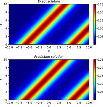
Figure 17. The exact double soliton solution (top) and learned solution (bottom) of the CDGSK equation. |
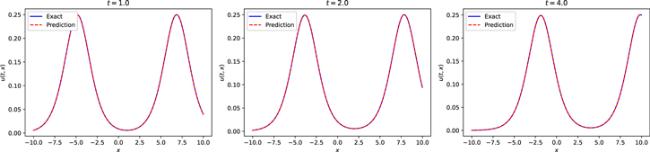
Figure 18. Comparison of the exact double soliton solution of the CDGSK equation and the approximate solution of the neural network at different times. |
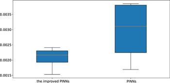
Figure 19. Error statistics for the improved PINNs and the original PINNs for solving double soliton solutions of the CDGSK equation. |
3.4. The numerical solution for fractal solitons waves of the p-gBKP equation
In recent years, fractal solitary waves have received more and more attention, and a large number of scholars have carried out studies on the complex propagation phenomenon of fractal solitary waves [62–64]. For example, He et al [65] studied the fractal Korteweg–de Vries (KdV) equation to obtain its solitary wave solution and discovered the solution properties of solitary waves moving along an unsmooth boundary, revealing that the peak of the solitary wave is weakly influenced by the unsmooth boundary. Wu et al [66] studied the fractal variant of the Boussinesq-Burgers equation and found that the order of the fractal derivative has a significant effect on the propagation process of the solitary wave, while it has less effect on the whole shape of the solitary wave. In this section, the fractal solitons waves of the p-gBKP equation [67] are studied. The mathematical form of the p-gBKP equation is defined as follows:
$\begin{eqnarray}\begin{array}{l}-\displaystyle \frac{9}{8}{u}_{x}{u}^{2}v-\displaystyle \frac{3}{8}{u}^{3}{u}_{y}-\displaystyle \frac{3}{4}{u}_{{xx}}{uv}-\displaystyle \frac{3}{4}{u}_{x}^{2}v-\displaystyle \frac{9}{4}{u}_{x}{{uu}}_{y}\\ -\displaystyle \frac{3}{4}{u}^{2}{u}_{{yx}}-\displaystyle \frac{3}{2}{u}_{{xx}}{u}_{y}-\displaystyle \frac{3}{2}{u}_{x}{u}_{{yx}}+{u}_{{yt}}+3{u}_{{yx}}=0.\end{array}\end{eqnarray}$
In the above equation, $u_y=v_x$. Next, the fractal solitons waves of the p-gBKP equation will be studied based on the improved PINNs. The initial condition is given as follows:
$\begin{eqnarray}\begin{array}{l}u(0,x)\\ =\,\displaystyle \frac{4{A}_{2,3}\left({A}_{1,4}{A}_{x,1}+{A}_{2,4}{A}_{x,2}\cos \left({A}_{x,2}x+{b}_{2}\right)\right)\left({\xi }_{2}{A}_{2,3}-{A}_{2,4}{\xi }_{1}\right)}{\left({A}_{2,3}^{2}{\xi }_{2}{}^{2}-{A}_{2,4}^{2}{\xi }_{1}{}^{2}\right)}\end{array}\end{eqnarray}$
$\begin{eqnarray}\left\{\begin{array}{c}{\xi }_{1}=\displaystyle \frac{{A}_{2,3}{A}_{1,4}\left({{xA}}_{x,1}+{{yA}}_{y,1}+{b}_{1}\right)}{{A}_{2,4}}+{A}_{2,3}\sin \left({A}_{x,2}x+{b}_{2}\right)+{b}_{3}\\ {\xi }_{2}={A}_{1,4}\left({{xA}}_{x,1}+{{yA}}_{y,1}+{b}_{1}\right)+{A}_{2,4}\sin \left({A}_{x,2}x+{b}_{2}\right)+{b}_{4}\end{array}\right..\end{eqnarray}$
In the above equation, the parameters take the following values
$\begin{eqnarray}\begin{array}{ccc}{A}_{1,4} & = & 2,{\unicode{x000A0}}{A}_{2,3}=2,{\unicode{x000A0}}{A}_{2,4}=3,{\unicode{x000A0}}{A}_{x,1}=23,\\ {A}_{x,2} & = & 2,{\unicode{x000A0}}{A}_{y,1}=2,{b}_{1}=1,{\unicode{x000A0}}{b}_{2}=1,{\unicode{x000A0}}{b}_{3}=1,{\unicode{x000A0}}{b}_{4}=1.\end{array}\end{eqnarray}$
In addition, the spatial range is [−30, 30], and the time range is [0, 5]. Under the above conditions, the fractal soliton wave of the p-gBKP equation is given as follows:
$\begin{eqnarray}u=\displaystyle \frac{4{A}_{\mathrm{2,3}}\left({A}_{\mathrm{1,4}}{A}_{x,1}+{A}_{\mathrm{2,4}}{A}_{x,2}\cos \left(3{{tA}}_{x,2}-{A}_{x,2}x-{b}_{2}\right)\right)\left({\xi }_{2}{A}_{\mathrm{2,3}}-{A}_{\mathrm{2,4}}{\xi }_{1}\right)}{\left({A}_{2,3}^{2}{\xi }_{2}{}^{2}-{A}_{2,4}^{2}{\xi }_{1}{}^{2}\right)},\end{eqnarray}$
$\begin{eqnarray}\left\{\begin{array}{l}{\xi }_{1}=\displaystyle \frac{{A}_{\mathrm{2,3}}{A}_{\mathrm{1,4}}\left(-3{{tA}}_{x,1}+{{xA}}_{x,1}+{{yA}}_{y,1}+{b}_{1}\right)}{{A}_{\mathrm{2,4}}}-{A}_{\mathrm{2,3}}\sin \left(3{{tA}}_{x,2}-{A}_{x,2}x-{b}_{2}\right)+{b}_{3}\\ {\xi }_{2}={A}_{\mathrm{1,4}}\left(-3{{tA}}_{x,1}+{{xA}}_{x,1}+{{yA}}_{y,1}+{b}_{1}\right)-{A}_{\mathrm{2,4}}\sin \left(3{{tA}}_{x,2}-{A}_{x,2}x-{b}_{2}\right)+{b}_{4}\end{array}\right..\end{eqnarray}$
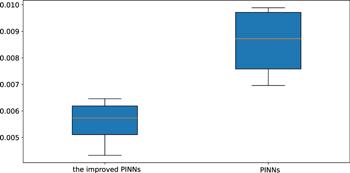
Next, we build a neural network with 9 hidden layers, where the number of neurons in the hidden layer is 32, and the activation function is still an adaptive activation function. For the initial condition, it is still regarded as a special type of Dirichlet boundary condition in the space-time domain. The training data regarding the initial and boundary conditions were obtained by random sampling with a sample size of 600. Residual points are randomly selected in the space-time domain to construct physical constraints, and the amount of data sampled in this experiment is 20 000. In addition, a small number of observations are used, the number of observations being 600. During training, the learning rate is set to 0.001, and L-BFGS is used to complete 5000 epoch iterations, and then Adam is used to continue the optimization until convergence. After training, we use the trained model to approximate the fractal soliton wave of the p-gBKP equation. In order to further analyze the experimental results intuitively, the prediction results are selected to be compared with the exact solution to check the accuracy of the prediction results. Figure 20 shows the exact solution and the predicted results using the trained model with t = 5. As can be seen from the figure, the neural network successfully simulates the fractal soliton wave of the p-gBKP equation. It can be seen that the prediction result is very close to the true solution. In addition, the error between the approximate solution and the exact solution is counted through many experiments, and the relative L2 norm error between the prediction results and the exact solution is about 5.56 × 10⁻³. Under the same training data and parameter settings, the relative L2 norm error between the prediction results calculated by the original PINNs and the exact solution is about 8.58 × 10⁻³. Figure 21 shows the error statistics of the improved PINNs and the original PINNs. Finally, the training time was analysed again and it was found that the average time to complete the training task for the improved PINNs was approximately 62.5% of the training time for the original PINNs. Experiments show that the improved PINN is more efficient in training than the original PINNs for the fractal soliton wave simulation problem of the p-gBKP equation.
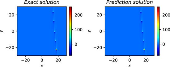
Figure 20. The exact solution (left) and learned solution (right) of the p-gBKP equation with t = 5. |
Figure 21. Error statistics for the improved PINNs and the original PINNs for solving the fractal solitons waves of the p-gBKP equation. |
4. Conclusion
In this paper, we have applied the improved PINNs to the numerical simulation of solitary wave solutions of several PDEs. The improved PINNs not only combine the constraints of the PDEs to ensure the interpretability of the prediction results, but also introduce the adaptive activation function, which introduces hyperparameters in the activation function to change the slope of the activation function to avoid gradient disappearance, thus saving computation time and speeding up the training. In the experiments, the mKdV equation, the improved Boussinesq equation, the CDGSK equation, and the p-gBKP equation are selected for study, and the errors of the results are analyzed to assess the accuracy of the predicted solitary wave solutions. The experimental results show that the improved PINNs significantly outperform the original PINNs with shorter training time and more accurate prediction results. The modified PINNs improve the training speed by more than 1.5 times compared with the classical PINNs, while maintaining the prediction error of less than the order of 10−2. Furthermore, with fractal solitary solutions and their applications attracting much attention from researchers, an exploratory study of related problems is conducted in this paper, and the results show that the method of this paper has good applicability to the simulation of fractal solitary waves. In our next work, we will further extend the method of this paper and carry out in-depth research on PDEs of fractal order and their solitary wave solutions. As the modified PINNs can simulate solitary wave phenomena well, we will try to extend and apply them to problems such as ocean wave simulation. In addition, there are many issues worth exploring in PINNs, such as how to better set the weight coefficients of different loss terms and how to solve the possible non-convergence problems in the optimization of loss functions, which will be explored and analyzed in depth in our next studies.