


1. Introductions
2. Constraint to the Lagrange multiplier and BRST quantization
2.1. Additional constraint
2.2. Gauge symmetry
2.3. BRST quantization
| 1. | (1) Because the BRST symmetry is a global symmetry with respect to the fermionic constant ε, one can define the conservation fermionic charge from Nother’s theorem $\begin{eqnarray}Q=\displaystyle \sum _{i}{u}_{i}({\dot{\lambda }}_{i}/\xi +{T}_{i})-\displaystyle \sum _{i}{\dot{u}}_{i}\displaystyle \frac{\delta }{\delta {\lambda }_{i}}.\end{eqnarray}$ All the physical states which are ghost-free obey $\begin{eqnarray}Q| \mathrm{Phys}\rangle =0.\end{eqnarray}$ This recovers Ti = 0 and ${\dot{\lambda }}_{i}(t)=0$ because ξ is an arbitrary constant. From the gauge theory point of view, ${\lambda }_{i}(t)=\bar{\lambda }$ is also a GFC, which removes the redundant degrees of freedom but the constraint Ti = 0 is relaxed to ⟨Ti⟩ = 0. This brings other unphysical degrees of freedom into the quantum state space. The gauge theory developed in [18–21] tried to solve this problem in a different way from ours. |
| 2. | (2) The nilpotency Q2 = 0 resembles the external differential operator d2 = 0 in the deRahm cohomology. The constraint ( |
| 3. | (3) Introducing the ghost fields greatly simplifies the quantization of the non-Abelian gauge theory which we will not involve in here. For the Abelian gauge theory considered in this paper, the ghost fields are decoupled to the gauge field and can be integrated away. Therefore, we will use the path integral ( $\begin{eqnarray}Z=\int \displaystyle \prod _{i,\tau }{\rm{d}}{{\rm{\Phi }}}_{i}^{\dagger }(\tau ){\rm{d}}{{\rm{\Phi }}}_{i}(\tau ){\rm{d}}{\lambda }_{i}(\tau ){{\rm{e}}}^{-{\int }_{0}^{\beta }{\rm{d}}\tau {L}_{\mathrm{eff}}},\end{eqnarray}$ where β = 1/T and ${\dot{\lambda }}_{i}(\tau )\equiv {\partial }_{\tau }\lambda (\tau )$. |
3. The Hubbard model at half-filling
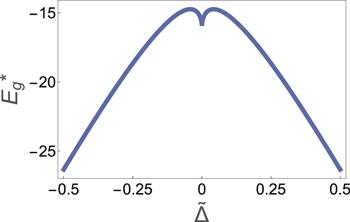
Figure 1. Numerical result of ${E}_{g}^{* }$ of $\tilde{{\rm{\Delta }}}$. We choose the dispersion of the normal state to be ${\xi }_{{\boldsymbol{k}}}=-t(\cos {k}_{x}+\cos {k}_{y})-{\mu }_{f}$, with t = 0.5 and μf = − 0.01. |
4. t–J model
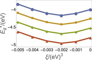
Figure 2. Numerical result of ${E}_{{\rm{g}}}^{* }$ of ξ. We choose the material data of cuprates [44], i.e. J ∼ 0.12 eV, χf ∼ 0.2 − 0.3, ρh ∼ 0.18 − 0.25, and μf ∼ −0.05 eV. The four curves in the diagram, from the top to bottom, correspond to Jχf/4 + tρh = 0.10 eV, 0.11 eV, 0.12 eV, and 0.13 eV, respectively. |