


1. Introduction
Quantum entanglement is one type of significant resource. Many kinds of quantum cryptographic protocols utilizing entanglement have been proposed, such as quantum secure direct communication [1], quantum network coding [2–5], and quantum operation sharing [6–8]. As we all know, remote state preparation (RSP), as an important application of quantum entanglement, was first proposed by Lo [9] for the transmission of pure known states. In RSP, the information of the desired state is known to the sender, while it may cause information leakage in the process of information transmission. Therefore, multi-party RSP has been investigated to enhance security, such as joint remote state preparation [10–13] and controlled remote state preparation [14–17]. In addition, bidirectional RSP [18–21], hierarchical RSP [22–24] and RSP in noisy environments [25, 26] have been studied.
To better satisfy the needs of quantum communication, Sang et al [27] proposed a protocol for controlled tripartite remote preparation by utilizing a seven-qubit entangled channel, in which three single-qubit states were prepared deterministically. Wang et al [28] then proposed a controlled cyclic remote state preparation (CCRSP) protocol of arbitrary-qubit states. Zha et al [29] presented a novel deterministic controlled tripartite remote preparation scheme for arbitrary single-qubit states via a seven-qubit entangled state. Peng et al [30] proposed a scheme for cyclic remote state preparation (CRSP) of arbitrary single-qubit states using a six-qubit entangled state, and it can also be extended to systems with n senders, allowing for the cyclic preparation of quantum states in different directions. Afterward, Zhang et al [31] presented a cyclic joint remote state preparation (CJRSP) protocol by using three Greenberger-Home-Zeilinger (GHZ) states, and further generalized it from three senders to n senders. They also discussed the protocol in amplitude-damping noisy environment. Sang [32] put forward a scheme of controlled CJRSP for arbitrary single-qubit states by sharing a ten-qubit entangled channel. Furthermore, Shi [33] proposed a scheme for unidirectional CCRSP of single-qutrit equatorial states via a seven-qutrit entangled state. Ma et al [34] also proposed a novel protocol for CCRSP of single-qutrit equatorial states. In addition to these mentioned protocols for cyclically preparing arbitrary single-qubit states, Sun et al [35] presented a protocol for cyclically preparing arbitrary two-qubit states and studied two-type quantum noises. Other protocols for cyclic remote preparation had been also proposed, such as multi-hop [36] and asymmetric [37] CRSP schemes.
Inspired by the above works, we first propose a scheme for CCRSP of arbitrary single-qubit states among three senders by utilizing a seven-qubit entangled state. In the scheme, it is assumed that the senders cannot communicate with each other through a classical channel, but they just communicate with the controller. Under the assistance of the controller, one sender could prepare an arbitrary single-qubit state for another in one direction. Only if all the participants cooperate can the three single-qubit states be prepared successfully. It is worthwhile to say that all senders are not required to employ information splitting and additional unitary operations before making measurements, owing to the ingenious construction of the measurement basis. Moreover, we generalize the CCRSP from three senders to the case of n senders and propose a universal protocol for multi-party CCRSP that can transmit n arbitrary single-qubit states at one time in the quantum network. Furthermore, in light of the influence of the actual environment, we study the impact of five-type quantum noises on the proposed CCRSP scheme with three senders. To better analyze the influence of quantum noise, fidelity is utilized to describe the closeness between the output states and the original states. The result indicates that fidelity is related to the coefficients of the prepared states and the noise parameters. The higher the fidelity, the better the communication quality, and the less information is lost.
The remainder of our paper is arranged as follows. In section 2 , we propose a CCRSP protocol with three senders. In section 3 , a universal multi-party CCRSP protocol with n senders is presented. We then offer some discussions and comparisons in section 4 . In section 5 , we study the effect of quantum noise on the proposed scheme in section 2 . Last, we summarize our work in section 6 .
2. CCRSP scheme with three senders
In this section, a protocol for cyclically preparing arbitrary single-qubit states in one direction among three senders is proposed. With the aid of one controller Charlie, the sender Alice1 wants to help Alice2 prepare an arbitrary single-qubit state ∣φ1⟩, Alice2 wishes to prepare an arbitrary single-qubit state ∣φ2⟩ for Alice3, and Alice3 desires to prepare an arbitrary single-qubit state ∣φ3⟩ at Alice1's site. Note that these senders are also receivers. For convenience, the arbitrary single-qubit state is indicated as
$\begin{eqnarray}| {\phi }_{j}\rangle ={\alpha }_{j}| 0\rangle +{\beta }_{j}| 1\rangle ,\end{eqnarray}$
where αj denotes a real number, βj denotes a complex number, and they also obey the normalization condition ∣αj∣2 + ∣βj∣2 = 1, j = 1, 2, 3. The sender Alicej grasps the coefficients of state ∣φj⟩, but the receiver ${\mathrm{Alice}}_{j+1(\mathrm{mod}\,3)}$ knows nothing about it.Suppose that the three senders and the controller Charlie pre-share a seven-qubit entangled channel
$\begin{eqnarray}\begin{array}{rcl}| {\rm{\Omega }}\rangle & = & \displaystyle \frac{1}{\sqrt{2}}\left[| {\varphi }^{+}{\rangle }_{\mathrm{1,2}}\otimes | {\varphi }^{+}{\rangle }_{\mathrm{3,4}}\otimes | {\varphi }^{+}{\rangle }_{\mathrm{5,6}}\otimes | 0{\rangle }_{7}\right.\\ & & \left.+| {\varphi }^{-}{\rangle }_{\mathrm{1,2}}\otimes | {\varphi }^{-}{\rangle }_{\mathrm{3,4}}\otimes | {\varphi }^{-}{\rangle }_{\mathrm{5,6}}\otimes | 1{\rangle }_{7}\right],\end{array}\end{eqnarray}$
where $| {\varphi }^{\pm }\rangle =\tfrac{1}{\sqrt{2}}(| 00\rangle \pm | 11\rangle )$, Alice1 processes qubits (1, 6), Alice2 holds qubits (2, 3), Alice3 owns qubits (4, 5), and qubit 7 belongs to Charlie. To complete our protocol, Alice1, Alice2, Alice3 and Charlie need to work together to perform the following operations.Step 1. The sender Alicej (j = 1, 2, 3) introduces an auxiliary particle $| 0{\rangle }_{(2j-1)^{\prime} }$ locally, and then employs a Controlled-Not (CNOT) operation ${C}_{(2j-1),(2j-1)^{\prime} }$, where the qubit (2j − 1) works as the controlled qubit, and the qubit $(2j-1)^{\prime} $ as the goal qubit. Then the quantum channel ∣Ω⟩ transforms into
$\begin{eqnarray}\begin{array}{rcl}| {\rm{\Omega }}^{\prime} \rangle & = & \displaystyle \frac{1}{4}\left[{\left(| 000\rangle +| 111\rangle \right)}_{\mathrm{1,1}^{\prime} ,2}\otimes {\left(| 000\rangle +| 111\rangle \right)}_{\mathrm{3,3}^{\prime} ,4}\right.\\ & & \otimes \,{\left(| 000\rangle +| 111\rangle \right)}_{\mathrm{5,5}^{\prime} ,6}\otimes | 0{\rangle }_{7}\\ & & +\,{\left(| 000\rangle -| 111\rangle \right)}_{\mathrm{1,1}^{\prime} ,2}\otimes {\left(| 000\rangle -| 111\rangle \right)}_{\mathrm{3,3}^{\prime} ,4}\\ & & \left.\otimes {\left(| 000\rangle -| 111\rangle \right)}_{\mathrm{5,5}^{\prime} ,6}\otimes | 1{\rangle }_{7}\right].\end{array}\end{eqnarray}$
Step 2 Alicej employs a two-qubit projective measurement on qubits $[(2j-1),(2j-1)^{\prime} ]$ under the basis $\{| {\eta }_{00}^{j}\rangle ,| {\eta }_{10}^{j}\rangle ,| {\eta }_{01}^{j}\rangle ,| {\eta }_{11}^{j}\rangle \}$:
$\begin{eqnarray}\left(\begin{array}{c}| {\eta }_{00}^{j}\rangle \\ | {\eta }_{10}^{j}\rangle \\ | {\eta }_{01}^{j}\rangle \\ | {\eta }_{11}^{j}\rangle \end{array}\right)=\displaystyle \frac{1}{\sqrt{2}}{\left(\begin{array}{cccc}{\alpha }_{j} & {\beta }_{j} & {\alpha }_{j} & {\beta }_{j}\\ {\alpha }_{j} & {\beta }_{j}^{* } & -{\alpha }_{j} & -{\beta }_{j}^{* }\\ {\beta }_{j}^{* } & -{\alpha }_{j} & {\beta }_{j}^{* } & -{\alpha }_{j}\\ {\beta }_{j} & -{\alpha }_{j} & -{\beta }_{j} & {\alpha }_{j}\end{array}\right)}^{\dagger }\left(\begin{array}{c}| 00\rangle \\ | 10\rangle \\ | 01\rangle \\ | 11\rangle \end{array}\right).\end{eqnarray}$
Alicej then transmits the measurement result in the form of classical messages sjtj (sj, tj ∈ {0, 1}) to Charlie through the classical channel.Based upon the measurement bases {$| {\eta }_{{s}_{1}{t}_{1}}^{1}{\rangle }_{\mathrm{1,1}^{\prime} }$, {$| {\eta }_{{s}_{2}{t}_{2}}^{2}{\rangle }_{\mathrm{3,3}^{\prime} }$ and {$| {\eta }_{{s}_{3}{t}_{3}}^{3}{\rangle }_{\mathrm{5,5}^{\prime} }$, we can rewrite the state $| {\rm{\Omega }}^{\prime} \rangle $ as
$\begin{eqnarray}\begin{array}{l}| {\rm{\Omega }}^{\prime} \rangle =\displaystyle \frac{1}{8\sqrt{2}}\displaystyle \sum _{{s}_{1},{t}_{1},{s}_{2},{t}_{2},{s}_{3},{t}_{3}=0}^{1}\left(\underset{j=1}{\overset{3}{\bigotimes }}| {\eta }_{{s}_{j}{t}_{j}}^{j}{\rangle }_{(2j-1)(2j-1)^{\prime} }\right)\\ \,\times | {{\rm{\Phi }}}_{{s}_{1}{t}_{1}{s}_{2}{t}_{2}{s}_{3}{t}_{3}}{\rangle }_{\mathrm{2,4},\mathrm{6,7}},\end{array}\end{eqnarray}$
where $| {{\rm{\Phi }}}_{{s}_{1}{t}_{1}{s}_{2}{t}_{2}{s}_{3}{t}_{3}}{\rangle }_{\mathrm{2,4},\mathrm{6,7}}$ is the composite state of qubits (2, 4, 6, 7), and it can be expressed as $\begin{eqnarray}\begin{array}{l}| {{\rm{\Phi }}}_{{s}_{1}{t}_{1}{s}_{2}{t}_{2}{s}_{3}{t}_{3}}{\rangle }_{\mathrm{2,4},\mathrm{6,7}}=\displaystyle \sum _{k=0}^{1}\\ \quad \times \left(\underset{j=1}{\overset{3}{\displaystyle \bigotimes }}{\left(-1\right)}^{{s}_{j}({t}_{j}\oplus k)}\left[{\left(-1\right)}^{{s}_{j}}{\alpha }_{j}| {s}_{j}\rangle \right.\right.\\ \quad \left.{\left.+{\left(-1\right)}^{{t}_{j}\oplus k}{\beta }_{j}| 1-{s}_{j}\rangle \right]}_{2j}\Space{0ex}{3.25ex}{0ex}\right)| k{\rangle }_{7},\end{array}\end{eqnarray}$
where ⊕ is an addition mod 2.Step 3. If Charlie desires to help Alicej, he is required to perform one single-qubit measurement under the Z basis $\left\{| l\rangle ,l\in \{0,1\}\right\}$. Depending on the received classical messages, Charlie just transmits two-bit classical messages (sP(j+1),tP(j+1) ⊕ l) to ${\mathrm{Alice}}_{j+1(\mathrm{mod}\,3)}$ respectively by making use of network coding. Here P is the cycling permutation (1, 2, 3).
If Charlie gets the measurement result ∣0⟩, the state of qubits (2,4,6) will collapse into
$\begin{eqnarray}\underset{j=1}{\overset{3}{\bigotimes }}{\left(-1\right)}^{{s}_{j}{t}_{j}}{\left[{\left(-1\right)}^{{s}_{j}}{\alpha }_{j}| {s}_{j}\rangle +{\left(-1\right)}^{{t}_{j}}{\beta }_{j}| 1-{s}_{j}\rangle \right]}_{2j}.\end{eqnarray}$
While if Charlie's measurement result is ∣1⟩, the collapsed state is expressed as $\begin{eqnarray}\underset{j=1}{\overset{3}{\bigotimes }}{\left(-1\right)}^{{s}_{j}({t}_{j}\oplus 1)}{\left[{\left(-1\right)}^{{s}_{j}}{\alpha }_{j}| {s}_{j}\rangle +{\left(-1\right)}^{{t}_{j}\oplus 1}{\beta }_{j}| 1-{s}_{j}\rangle \right]}_{2j}.\end{eqnarray}$
Step 4. According to the classical messages received, ${\mathrm{Alice}}_{j+1(\mathrm{mod}\,3)}$ (j = 1, 2, 3) executes the recovery operation9 ) on the collapsed state of equations (7 ) and (8 ), Alicej can always be capable of recovering the desired state with unit success probability.
$\begin{eqnarray}{R}_{{A}_{j+1(\mathrm{mod}\,3)}}\ \ ={X}^{{s}_{P(j+1)}}\ \ {Z}^{{s}_{P(j+1)}\ \ \oplus {t}_{P(j+1)}\ \ \oplus l}\end{eqnarray}$
on her qubit to obtain the goal state ∣φj⟩. Here X and Z are Pauli operators, and X0 = Z0 = I. In a word, by employing suitable recovery operations of equation (In practice, there are a total of 128 types of measurement outcomes, however, we just list partial recovery operations in the case that Alice1's measurement result is $| {\eta }_{00}^{1}\rangle $ in table 1, where ${M}_{{A}_{j}}$ and MC are the measurement outcomes of Alicej and Charlie. ${R}_{{A}_{j}}$ denotes Alicej's recovery unitary operation.
Table 1. The relation between the partial measurement results $({M}_{{A}_{2}}$, ${M}_{{A}_{3}},{M}_{C})$ of three participants and recovery unitary operations $({R}_{{A}_{1}}{R}_{{A}_{2}}{R}_{{A}_{3}})$ when ${M}_{{A}_{1}}$ is $| {\eta }_{00}^{1}\rangle $. |
| ${M}_{{A}_{2}}$ | ${M}_{{A}_{3}}$ | MC | ${R}_{{A}_{1}}{R}_{{A}_{2}}{R}_{{A}_{3}}$ | MC | ${R}_{{A}_{1}}{R}_{{A}_{2}}{R}_{{A}_{3}}$ |
|---|---|---|---|---|---|
| $| {\eta }_{00}^{2}\rangle $ | $| {\eta }_{00}^{3}\rangle $ | ∣0⟩ | I6I2I4 | ∣1⟩ | Z6Z2Z4 |
| $| {\eta }_{00}^{2}\rangle $ | $| {\eta }_{10}^{3}\rangle $ | ∣0⟩ | Y6I2I4 | ∣1⟩ | X6Z2Z4 |
| $| {\eta }_{00}^{2}\rangle $ | $| {\eta }_{01}^{3}\rangle $ | ∣0⟩ | Z6I2I4 | ∣1⟩ | I6Z2Z4 |
| $| {\eta }_{00}^{2}\rangle $ | $| {\eta }_{11}^{3}\rangle $ | ∣0⟩ | X6I2I4 | ∣1⟩ | Y6Z2Z4 |
| | |||||
| $| {\eta }_{10}^{2}\rangle $ | $| {\eta }_{00}^{3}\rangle $ | ∣0⟩ | I6I2Y4 | ∣1⟩ | Z6Z2X4 |
| $| {\eta }_{10}^{2}\rangle $ | $| {\eta }_{10}^{3}\rangle $ | ∣0⟩ | Y6I2Y4 | ∣1⟩ | X6Z2X4 |
| $| {\eta }_{10}^{2}\rangle $ | $| {\eta }_{01}^{3}\rangle $ | ∣0⟩ | Z6I2Y4 | ∣1⟩ | I6Z2X4 |
| $| {\eta }_{10}^{2}\rangle $ | $| {\eta }_{11}^{3}\rangle $ | ∣0⟩ | X6I2Y4 | ∣1⟩ | Y6Z2X4 |
| | |||||
| $| {\eta }_{01}^{2}\rangle $ | $| {\eta }_{00}^{3}\rangle $ | ∣0⟩ | I6I2Z4 | ∣1⟩ | Z6Z2I4 |
| $| {\eta }_{01}^{2}\rangle $ | $| {\eta }_{10}^{3}\rangle $ | ∣0⟩ | Y6I2Z4 | ∣1⟩ | X6Z2I4 |
| $| {\eta }_{01}^{2}\rangle $ | $| {\eta }_{01}^{3}\rangle $ | ∣0⟩ | Z6I2Z4 | ∣1⟩ | I6Z2I4 |
| $| {\eta }_{01}^{2}\rangle $ | $| {\eta }_{11}^{3}\rangle $ | ∣0⟩ | X6I2Z4 | ∣1⟩ | Y6Z2I4 |
| | |||||
| $| {\eta }_{11}^{2}\rangle $ | $| {\eta }_{00}^{3}\rangle $ | ∣0⟩ | I6I2X4 | ∣1⟩ | Z6Z2Y4 |
| $| {\eta }_{11}^{2}\rangle $ | $| {\eta }_{10}^{3}\rangle $ | ∣0⟩ | Y6I2X4 | ∣1⟩ | X6Z2Y4 |
| $| {\eta }_{11}^{2}\rangle $ | $| {\eta }_{01}^{3}\rangle $ | ∣0⟩ | Z6I2X4 | ∣1⟩ | I6Z2Y4 |
| $| {\eta }_{11}^{2}\rangle $ | $| {\eta }_{11}^{3}\rangle $ | ∣0⟩ | X6I2X4 | ∣1⟩ | Y6Z2Y4 |
A specific example is given below to clearly illustrate our scheme. Generally, we assume that Alice1's, Alice2's and Alice3's measurement results are $| {\eta }_{00}^{1}\rangle $, $| {\eta }_{01}^{2}\rangle $ and $| {\eta }_{10}^{3}\rangle $, then qubits (2, 4, 6, 7) collapse into
$\begin{eqnarray}\begin{array}{l}| {\rm{\Phi }}{\rangle }_{\mathrm{2,4},\mathrm{6,7}}={\left({\alpha }_{1}| 0\rangle +{\beta }_{1}| 1\rangle \right)}_{2}\otimes {\left({\alpha }_{2}| 0\rangle -{\beta }_{2}| 1\rangle \right)}_{4}\\ \quad \otimes \,{\left({\beta }_{3}| 0\rangle -{\alpha }_{3}| 1\rangle \right)}_{6}\otimes | 0{\rangle }_{7}\\ \quad +{\left({\alpha }_{1}| 0\rangle -{\beta }_{1}| 1\rangle \right)}_{2}\otimes {\left({\alpha }_{2}| 0\rangle +{\beta }_{2}| 1\rangle \right)}_{4}\\ \quad \otimes \,{\left({\beta }_{3}| 0\rangle +{\alpha }_{3}| 1\rangle \right)}_{6}\otimes | 1{\rangle }_{7}.\end{array}\end{eqnarray}$
If Charlie obtains the measurement outcome ∣1⟩, thus the state of qubits (2, 4, 6) collapses into
$\begin{eqnarray}\begin{array}{l}| {\rm{\Phi }}{\rangle }_{\mathrm{2,4,6}}={\left({\alpha }_{1}| 0\rangle -{\beta }_{1}| 1\rangle \right)}_{2}\otimes \left({\alpha }_{2}| 0\rangle \right.\\ \quad {\left.+{\beta }_{2}| 1\rangle \right)}_{4}\otimes {\left({\beta }_{3}| 0\rangle +{\alpha }_{3}| 1\rangle \right)}_{6}.\end{array}\end{eqnarray}$
Alice1, Alice2 and Alice3 execute Pauli operations X6, Z2 and I4 on their qubits 6, 2, 4, respectively, thus the desired single-qubit states ∣φ3⟩, ∣φ1⟩ and ∣φ2⟩ are reconstructed successfully.
3. CCRSP scheme with multiple senders
In this section, we present a deterministic multi-party CCRSP protocol of arbitrary single-qubit states for the case of n senders.
Alice1 wants to help Alice2 prepare an arbitrary single-qubit state ∣φ1⟩, Alice2 wishes to help Alice3 prepare an arbitrary single-qubit state ∣φ2⟩, ⋯, Alicen desires to prepare an arbitrary single-qubit state ∣φn⟩ for Alice1. The single-qubit state ∣φj⟩ (j = 1, 2, ⋯ ,n) is shown in equation (1 ), whereby the real numbers αj and complex numbers βj follow the normalization condition ∣αj∣2 + ∣βj∣2 = 1.
Assume Alice1, Alice2, ⋯, Alicen and Charlie pre-share a (2n + 1)-qubit entangled channel
$\begin{eqnarray}\begin{array}{rcl}| {C}_{2n+1}\rangle & = & \displaystyle \frac{1}{\sqrt{2}}\left[| {\varphi }^{+}{\rangle }_{\mathrm{1,2}}\otimes \cdots \otimes | {\varphi }^{+}{\rangle }_{2n-\mathrm{1,2}n}\otimes | 0{\rangle }_{2n+1}\right.\\ & & \left.+| {\varphi }^{-}{\rangle }_{\mathrm{1,2}}\otimes \cdots \otimes | {\varphi }^{-}{\rangle }_{2n-\mathrm{1,2}n}\otimes | 1{\rangle }_{2n+1}\right].\end{array}\end{eqnarray}$
Here Alicej processes qubits (2j − 2, 2j − 1), j = 2, 3, ⋯ ,n, and qubit 2n + 1 belongs to Charlie. In particular, Alice1 holds qubits (1, 2n). The specific process of the protocol are described in the following steps.Step 1. Alicej (j = 1, 2, ⋯ ,n) first introduces an auxiliary particle $| 0{\rangle }_{(2j-1)^{\prime} }$, and then employs a CNOT operation ${C}_{(2j-1),(2j-1)^{\prime} }$. The quantum channel ∣C2n+1⟩ then becomes
$\begin{eqnarray}\begin{array}{l}| {C}_{3n+1}\rangle ={\left(\displaystyle \frac{1}{\sqrt{2}}\right)}^{n+1}\left[{\left(| 000\rangle +| 111\rangle \right)}_{\mathrm{1,1}^{\prime} ,2}\otimes \cdots \right.\\ \quad \otimes {\left(| 000\rangle +| 111\rangle \right)}_{2n-1,(2n-1)^{\prime} ,2n}\otimes | 0{\rangle }_{2n+1}\\ \quad +{\left(| 000\rangle -| 111\rangle \right)}_{\mathrm{1,1}^{\prime} ,2}\otimes \cdots \\ \quad \left.\otimes {\left(| 000\rangle -| 111\rangle \right)}_{2n-1,(2n-1)^{\prime} ,2n}\otimes | 1{\rangle }_{2n+1}\right].\end{array}\end{eqnarray}$
Step 2. Alicej performs a two-qubit projective measurement on her qubits $[(2j-1),(2j-1)^{\prime} ]$ on the basis of equation (4 ). After the measurement, Alicej notifies Charlie classical message sjtj via the classical channel when the measurement result is $| {\eta }_{{s}_{j}{t}_{j}}^{j}\rangle $, (sj, tj ∈ {0, 1}).
In terms of measurement basis {$| {\eta }_{{s}_{j}{t}_{j}}^{j}{\rangle }_{(2j-1),(2j-1)^{\prime} }$, we reexpress the state ∣C3n+1⟩ as
$\begin{eqnarray}\begin{array}{l}| {C}_{3n+1}\rangle ={\left(\displaystyle \frac{1}{\sqrt{2}}\right)}^{2n+1}\displaystyle \sum _{{s}_{1},{t}_{1},\cdots {s}_{n},{t}_{n}=0}^{1}\\ \,\times \,\left(\underset{j=1}{\overset{n}{\bigotimes }}| {\eta }_{{s}_{j}{t}_{j}}^{j}{\rangle }_{(2j-1),(2j-1)^{\prime} }\right)| {{\rm{\Phi }}}_{{s}_{1}{t}_{1}\cdots {s}_{n}{t}_{n}}{\rangle }_{2,\cdots ,2n,2n+1},\end{array}\end{eqnarray}$
where the collapsed state of qubits (2, ⋯ ,2n, 2n + 1) can be expressed as $\begin{eqnarray}\begin{array}{l}| {{\rm{\Phi }}}_{{s}_{1}{t}_{1}\cdots {s}_{n}{t}_{n}}{\rangle }_{2,\cdots ,2n,2n+1}=\displaystyle \sum _{k=0}^{1}\left\{\underset{j=1}{\overset{n}{\bigotimes }}{\left(-1\right)}^{{s}_{j}({t}_{j}\oplus k)}\right.\\ \quad \left.\times {\left[{\left(-1\right)}^{{s}_{j}}{\alpha }_{j}| {s}_{j}\rangle +{\left(-1\right)}^{{t}_{j}\oplus k}{\beta }_{j}| 1-{s}_{j}\rangle \right]}_{2j}| k{\rangle }_{2n+1}\Space{0ex}{3.55ex}{0ex}\right\}.\end{array}\end{eqnarray}$
Step 3. To complete the task, Charlie employs a single-qubit measurement on his qubit under the Z basis. He then transmits two-bit classical messages (sP(j+1),tP(j+1) ⊕ l) to the receiver ${\mathrm{Alice}}_{j+1(\mathrm{mod}\,n)}$.
If Charlie obtains the measurement result as ∣0⟩, the qubits (2, 4, ⋯ ,2n) will collapse into
$\begin{eqnarray}\begin{array}{c}| {{\rm{\Phi }}}_{{s}_{1}{t}_{1}\cdots {s}_{n}{t}_{n}}{\rangle }_{2,\cdots ,2n}=\underset{j=1}{\overset{n}{\bigotimes }}{\left(-1\right)}^{{s}_{j}{t}_{j}}\left[{\left(-1\right)}^{{s}_{j}}{\alpha }_{j}| {s}_{j}\rangle \right.\\ \quad {\left.+{\left(-1\right)}^{{t}_{j}}{\beta }_{j}| 1-{s}_{j}\rangle \right]}_{2j},\end{array}\end{eqnarray}$
while if Charlie's measurement result is ∣1⟩, the collapsed state is $\begin{eqnarray}\begin{array}{l}| {{\rm{\Phi }}}_{{s}_{1}{t}_{1}\cdots {s}_{n}{t}_{n}}{\rangle }_{2,\cdots ,2n}=\underset{j=1}{\overset{n}{\bigotimes }}{\left(-1\right)}^{{s}_{j}({t}_{j}\oplus 1)}\\ \quad {\left[{\left(-1\right)}^{{s}_{j}}{\alpha }_{j}| {s}_{j}\rangle +{\left(-1\right)}^{{t}_{j}\oplus 1}{\beta }_{j}| 1-{s}_{j}\rangle \right]}_{2j}.\end{array}\end{eqnarray}$
Step 4 The receiver ${\mathrm{Alice}}_{j+1(\mathrm{mod}\,n)}$ (j = 1, 2, ⋯ ,n) performs the appropriate recovery operation ${R}_{{A}_{j+1(\mathrm{mod}\,n)}}$ in equation (9 ) and acquires the goal state
$\begin{eqnarray}\underset{j=1}{\overset{n}{\bigotimes }}({\alpha }_{j}| 0\rangle +{\beta }_{j}| 1\rangle ),\end{eqnarray}$
according to the classical messages they received, wherein P is the cycling permutation ${\left(1,n,n-1,\ldots ,2\right)}^{-1}$.As a consequence, Alice1, Alice2, ⋯, Alicen can deterministically construct n arbitrary single-qubit states ∣φn⟩, ∣φ1⟩, ⋯ ,∣φn−1⟩.
4. Discussions and comparisons
In this part, we first discuss the intrinsic efficiency [38] and the necessary operations of our universal protocol. After, we provide some comparisons with other protocols.
The intrinsic efficiency is a crucial factor for evaluating the performance of a protocol, which is defined by
$\begin{eqnarray}\eta =\displaystyle \frac{{q}_{s}}{{q}_{u}+{b}_{t}},\end{eqnarray}$
wherein qs represents the number of qubits teleported, qu denotes the number of particles used in the quantum channel, bt acts for the classical bits that need to be transmitted.As mentioned above, we propose a CCRSP scheme to simultaneously and deterministically prepare n arbitrary single-qubit states by sharing a (2n + 1)-qubit entangled channel. Alicej (j = 1, 2, ⋯ ,n) respectively transmit two classical bits to Charlie. Charlie encodes his classical message corresponding to his measurement outcome with the classical messages that he received from Alicej, and then sends the encoded results to ${\mathrm{Alice}}_{j+1(\mathrm{mod}\ n)}$. The total classical communication cost (CCC) is 4n classical bits. Thus, the intrinsic efficiency of our protocol is
$\begin{eqnarray}\eta =\displaystyle \frac{n}{(2n+1)+(4n)}=\displaystyle \frac{n}{6n+1}.\end{eqnarray}$
Specially, for our CCRSP protocol with three senders, the intrinsic efficiency is $\eta =\tfrac{3}{19}\approx 15.79 \% $.If network coding is not utilized, the total CCC is 5n bits. In this scenario, the intrinsic efficiency will be20 ), so the intrinsic efficiency of CCRSP protocol with three senders is $\eta =\tfrac{3}{25}\approx 13.64 \% $. It reveals that the utilization of network coding can effectively reduce the CCC and enhance the intrinsic efficiency.
$\begin{eqnarray}\eta =\displaystyle \frac{n}{(2n+1)+(5n)}=\displaystyle \frac{n}{7n+1},\end{eqnarray}$
which is lower than the intrinsic efficiency in equation (In the following, we present some comparisons with other CRSP protocols. To make the comparison convincing, we only choose a specific value n = 6. The results of comparisons with previous protocols are given in table 2. A detailed explanation of the abbreviations is provided as follows: QC (quantum channel), ES (entangled state), BO (basic operation), RUO (recovery unitary operation), SQM (single-qubit measurement), TQM (two-qubit measurement), CNOT (Controlled-NOT), NTQ (number of the teleported qubits).
From table 2, it can be seen that the intrinsic efficiency of [28, 30, 31] are all greater than ours. Besides their unfavorable aspects, our schemes also have advantages. In particular, adopting two-particle measurement instead of single-qubit measurement, the senders are not required to employ information splitting before performing measurements. The advantage is that two-qubit information can be obtained simultaneously in a single operation. Compared to the scheme in [28], their protocol failed in some cases of measurement results, but the success probability of ours can reach one, i.e. our protocol is deterministic. In comparison with the scheme in [30], our protocol has higher security, since the introduction of a controller can be effective in preventing a dishonest sender from not sending messages. Further, compared with the scheme in [31], five qubits are saved in the entangled channel, and fewer particles are exposed to noise during entanglement distribution. As a result, in comparison to other similar protocols, our protocol only increases the CCC but optimizes other aspects. Though it reduces the internal efficiency, the feasibility of our protocol is greatly improved.
5. The CCRSP scheme subjects to noisy environment
In real situations, however, quantum noise may have some influence on the quantum channel. It is general to assume that one of the participants is responsible for constructing the shared entanglement. The constructor then needs to send particles to each participant, and every particle to be transmitted will be inevitably affected by quantum noise during the distribution of entanglement. In what follows, we investigate the proposed CCRSP scheme in section 2 under five types of noises (bit-flip, phase-flip, bit-phase flip, amplitude-damping, and phase-damping noises).
5.1. Density operator representation of the CCRSP scheme
To better analyze the impact of quantum noise on the CCRSP protocol with three senders, it is convenient to redescribe the protocol in terms of density operators. Thus, the desired prepared states are denoted as ∣φ1⟩∣φ2⟩∣φ3⟩⟨φ3∣⟨φ2∣⟨φ1∣, and the quantum channel is shown as $\rho =| {\rm{\Omega }}^{\prime} \rangle \langle {\rm{\Omega }}^{\prime} | $. Alicej's (j = 1, 2, 3) and Charlie's measurement operators are ${M}_{{A}_{j}}=\left\{| {\eta }_{{s}_{j}{t}_{j}}^{j}\rangle \langle {\eta }_{{s}_{j}{t}_{j}}^{j}| ,{s}_{j},{t}_{j}\in \{0,1\}\right\}$ and ${M}_{C}=\left\{| 0\rangle \langle 0| ,| 1\rangle \langle 1| \right\}$. Hence, we redescribe the CCRSP scheme with three senders as follows.
Step 1. Alicej first introduces an auxiliary particle $| 0{\rangle }_{(2j-1)^{\prime} }$, and then executes a CNOT operation ${C}_{(2j-1),(2j-1)^{\prime} }$.
Step 2. Alice1 measures her qubits $(1,1^{\prime} )$ by measurement operators ${M}_{{A}_{1}}$ and the system of qubits $(2,3,3^{\prime} ,4,5,5^{\prime} ,6,7)$ turns to
$\begin{eqnarray}{\rho }_{1}={\mathrm{tr}}_{\mathrm{1,1}^{\prime} }\left(\displaystyle \frac{{M}_{{A}_{1}}\rho {M}_{{A}_{1}}^{\dagger }}{\mathrm{tr}({M}_{{A}_{1}}^{\dagger }{M}_{{A}_{1}}\rho )}\right).\end{eqnarray}$
Alice2 measures her qubits $(3,3^{\prime} )$ by measurement operators ${M}_{{A}_{2}}$ and the system of qubits $(2,4,5,5^{\prime} ,6,7)$ becomes
$\begin{eqnarray}{\rho }_{2}={\mathrm{tr}}_{\mathrm{3,3}^{\prime} }\left(\displaystyle \frac{{M}_{{A}_{2}}{\rho }_{1}{M}_{{A}_{2}}^{\dagger }}{\mathrm{tr}({M}_{{A}_{2}}^{\dagger }{M}_{{A}_{2}}{\rho }_{1})}\right).\end{eqnarray}$
Alice3 measures her qubits $(5,5^{\prime} )$ by measurement operators ${M}_{{A}_{3}}$ and the system of qubits (2, 4, 6, 7) collapses into
$\begin{eqnarray}{\rho }_{3}={\mathrm{tr}}_{\mathrm{5,5}^{\prime} }\left(\displaystyle \frac{{M}_{{A}_{3}}{\rho }_{2}{M}_{{A}_{3}}^{\dagger }}{\mathrm{tr}({M}_{{A}_{3}}^{\dagger }{M}_{{A}_{3}}{\rho }_{2})}\right).\end{eqnarray}$
Step 3. Charlie selects measurement operators MC for measuring his qubit 7, the system of qubits (2, 4, 6) becomes
$\begin{eqnarray}{\rho }_{4}={\mathrm{tr}}_{7}\left(\displaystyle \frac{{M}_{C}{\rho }_{3}{M}_{C}^{\dagger }}{\mathrm{tr}({M}_{C}^{\dagger }{M}_{C}{\rho }_{3})}\right).\end{eqnarray}$
Step 4. Alicej performs the unitary operation ${R}_{{A}_{j}}$ described in equation (9 ) and gets the output state
$\begin{eqnarray}{\rho }_{\mathrm{out}}=({R}_{{A}_{1}}{R}_{{A}_{2}}{R}_{{A}_{3}}){\rho }_{4}{\left({R}_{{A}_{1}}{R}_{{A}_{2}}{R}_{{A}_{3}}\right)}^{\dagger }.\end{eqnarray}$
5.2. Five types of quantum noises
The bit-flip, phase-flip and bit-phase flip noises are known as Pauli noises. The bit-flip noise refers to changing a qubit from ∣0⟩ to ∣1⟩ or ∣1⟩ to ∣0⟩ with probability λ. Interestingly, the phase-flip noise only changes the phase of qubit ∣1⟩ to −∣1⟩ with probability λ, while the phase of qubit ∣0⟩ remains unaffected. The bit-phase flip noise can be regarded as the combination of both the bit-flip and phase-flip noises, since σy = iσxσz. Their actions are denoted as Kraus operators [26]
$\begin{eqnarray}{E}_{0}^{\mathrm{bf}}=\sqrt{1-\lambda }I,\quad {E}_{1}^{\mathrm{bf}}=\sqrt{\lambda }{\sigma }_{x},\end{eqnarray}$
$\begin{eqnarray}{E}_{0}^{\mathrm{pf}}=\sqrt{1-\lambda }I,\quad {E}_{1}^{\mathrm{pf}}=\sqrt{\lambda }{\sigma }_{z},\end{eqnarray}$
$\begin{eqnarray}{E}_{0}^{\mathrm{bp}}=\sqrt{1-\lambda }I,\quad {E}_{1}^{\mathrm{bp}}=\sqrt{\lambda }{\sigma }_{y}.\end{eqnarray}$
The amplitude-damping (AD) and phase-damping (PD) noises are two types of important decoherence noises. The AD noise refers to the dissipation of energy in a quantum system, while the PD noise refers to the loss of quantum information without any energy loss, and their actions are shown by a set of Kraus operators [26]
$\begin{eqnarray}{E}_{0}^{{\rm{a}}}=\left(\begin{array}{cc}1 & 0\\ 0 & \sqrt{1-\lambda }\end{array}\right),\quad {E}_{1}^{{\rm{a}}}=\left(\begin{array}{cc}0 & \sqrt{\lambda }\\ 0 & 0\end{array}\right),\end{eqnarray}$
$\begin{eqnarray}\begin{array}{rcl}{E}_{0}^{{\rm{p}}} & = & \sqrt{1-\lambda }I,\quad {E}_{1}^{{\rm{p}}}=\begin{array}{c}\sqrt{\lambda }\end{array}\left(\begin{array}{cc}1 & 0\\ 0 & 0\end{array}\right),\\ {E}_{2}^{{\rm{p}}} & = & \begin{array}{c}\sqrt{\lambda }\end{array}\left(\begin{array}{cc}0 & 0\\ 0 & 1\end{array}\right),\end{array}\end{eqnarray}$
where λ(0 ≤ λ ≤ 1) indicates the decoherence rate of the five types of quantum noises.5.3. The output state and fidelity in a noisy environment
Without losing generality, suppose that the controller Charlie prepares the quantum channel ∣Ω⟩, then he distributes qubits (1, 6) to Alice1, qubits (2, 3) to Alice2, and qubits (4, 5) to Alice3 through the noisy environment. It is reasonable to introduce the auxiliary qubits locally via the senders, and they are not exposed to the noisy environment. Thus, we assume that the auxiliary particles used in local CNOT operations are not affected by quantum noise during the distribution of entanglement. Supposed that there is the same type of noise effect on each channel, the effect of noise on the shared channel ρ is expressed as22 ), and we can obtain the fidelity as
$\begin{eqnarray}\varepsilon (\rho )=\displaystyle \sum _{{j}_{1},{j}_{2},{j}_{3}}{E}_{{j}_{1}}^{1}{E}_{{j}_{1}}^{6}{E}_{{j}_{2}}^{2}{E}_{{j}_{2}}^{3}{E}_{{j}_{3}}^{4}{E}_{{j}_{3}}^{5}\rho {E}_{{j}_{1}}^{{1}^{\dagger }}{E}_{{j}_{1}}^{{6}^{\dagger }}{E}_{{j}_{2}}^{{2}^{\dagger }}{E}_{{j}_{2}}^{{3}^{\dagger }}{E}_{{j}_{3}}^{{4}^{\dagger }}{E}_{{j}_{3}}^{{5}^{\dagger }},\end{eqnarray}$
where the subscripts j1, j2, j3 denote the Kraus operator that is employed. In AD and Pauli noises, j1, j2, j3 ∈ {0, 1}, while in PD noise, j1, j2, j3 ∈ {0, 1, 2}. The superscripts 1, 6, 2, 3, 4, 5 denote which qubit that operator E acts on. To calculate the fidelity of the output state, we replace ρ by ϵ(ρ) in equation ( $\begin{eqnarray}F=\langle {\phi }_{1}| \langle {\phi }_{2}| \langle {\phi }_{3}| {\rho }_{\mathrm{out}}| {\phi }_{3}\rangle | {\phi }_{2}\rangle | {\phi }_{1}\rangle .\end{eqnarray}$
Here, we just take the measurement results $| {\eta }_{00}^{1}\rangle | {\eta }_{01}^{2}\rangle | {\eta }_{10}^{3}\rangle | 1\rangle $ as an example, and we show the impact of bit flip noise on the CCRSP in more detail. For convenience, denote $\widetilde{\lambda }=1-\lambda $. From equation (32 ), the effect of noise on the shared quantum channel $| {\rm{\Omega }}^{\prime} \rangle $ is
$\begin{eqnarray*}\begin{array}{rcl}{\varepsilon }_{\mathrm{bf}}(\rho ) & = & \displaystyle \frac{1}{16}\left\{{\lambda }^{6}\displaystyle \sum _{k=0}^{1}{\left(| 101\rangle +{\left(-1\right)}^{k}| 010\rangle \right)}^{\otimes 3}| k\rangle \right.\\ & & \times \displaystyle \sum _{k=0}^{1}{\left(\langle 101| +{\left(-1\right)}^{k}\langle 010| \right)}^{\otimes 3}\langle k| \\ & & +{\widetilde{\lambda }}^{6}\displaystyle \sum _{k=0}^{1}{\left(| 000\rangle +{\left(-1\right)}^{k}| 111\rangle \right)}^{\otimes 3}| k\rangle \\ & & \times \displaystyle \sum _{k=0}^{1}{\left(\langle 000| +{\left(-1\right)}^{k}\langle 111| \right)}^{\otimes 3}\langle k| \\ & & +{\lambda }^{2}{\widetilde{\lambda }}^{4}\left[\displaystyle \sum _{k=0}^{1}\left(| 000\rangle +{\left(-1\right)}^{k}| 111\rangle \right)\right.\\ & & \times \left(| 001\rangle +{\left(-1\right)}^{k}| 110\rangle \right)\left(| 100\rangle +{\left(-1\right)}^{k}| 011\rangle \right)| k\rangle \\ & & \times \displaystyle \sum _{k=0}^{1}\left(\langle 000| +{\left(-1\right)}^{k}\langle 111| \right)\left(\langle 001| +{\left(-1\right)}^{k}\langle 110| \right)\end{array}\end{eqnarray*}$
$\begin{eqnarray*}\begin{array}{rcl} & & \left(\langle 100| +{\left(-1\right)}^{k}\langle 011| \right)\langle k| \\ & & +\displaystyle \sum _{k=0}^{1}\left(| 001\rangle +{\left(-1\right)}^{k}| 110\rangle \right)\left(| 100\rangle +{\left(-1\right)}^{k}| 011\rangle \right)\\ & & \times \left(| 000\rangle +{\left(-1\right)}^{k}| 111\rangle \right)| k\rangle \\ & & \times \displaystyle \sum _{k=0}^{1}\left(\langle 001| +{\left(-1\right)}^{k}\langle 110| \right)\left(\langle 100| +{\left(-1\right)}^{k}\langle 011| \right)\\ & & \times \left(\langle 000| +{\left(-1\right)}^{k}\langle 111| \right)\langle k| \\ & & +\displaystyle \sum _{k=0}^{1}\left(| 100\rangle +{\left(-1\right)}^{k}| 011\rangle \right)\left(| 000\rangle +{\left(-1\right)}^{k}| 111\rangle \right)\\ & & \times \left(| 001\rangle +{\left(-1\right)}^{k}| 110\rangle \right)| k\rangle \\ & & \times \displaystyle \sum _{k=0}^{1}\left(\langle 100| +{\left(-1\right)}^{k}\langle 011| \right)\left(\langle 000| +{\left(-1\right)}^{k}\langle 111| \right)\\ & & \left.\times \left(\langle 001| +{\left(-1\right)}^{k}\langle 110| \right)\langle k| \Space{0ex}{2.5ex}{0ex}\right]\end{array}\end{eqnarray*}$
$\begin{eqnarray*}\begin{array}{rcl} & & +{\lambda }^{4}{\widetilde{\lambda }}^{2}\left[\displaystyle \sum _{k=0}^{1}\left(| 100\rangle +{\left(-1\right)}^{k}| 011\rangle \right)\right.\\ & & \times \left(| 001\rangle +{\left(-1\right)}^{k}| 110\rangle \right)\left(| 101\rangle +{\left(-1\right)}^{k}| 010\rangle \right)| k\rangle \\ & & \times \displaystyle \sum _{k=0}^{1}\left(\langle 100| +{\left(-1\right)}^{k}\langle 011| \right)\left(\langle 001| +{\left(-1\right)}^{k}\langle 110| \right)\\ & & \times \left(\langle 101| +{\left(-1\right)}^{k}\langle 010| \right)\langle k| \\ & & +\displaystyle \sum _{k=0}^{1}\left(| 101\rangle +{\left(-1\right)}^{k}| 010\rangle \right)\left(| 100\rangle +{\left(-1\right)}^{k}| 011\rangle \right)\end{array}\end{eqnarray*}$
$\begin{eqnarray}\begin{array}{rcl} & & \times \left(| 001\rangle +{\left(-1\right)}^{k}| 110\rangle \right)| k\rangle \\ & & \times \displaystyle \sum _{k=0}^{1}\left(\langle 101| +{\left(-1\right)}^{k}\langle 010| \right)\left(\langle 100| +{\left(-1\right)}^{k}\langle 011| \right)\\ & & \times \left(\langle 001| +{\left(-1\right)}^{k}\langle 110| \right)\langle k| \\ & & +\displaystyle \sum _{k=0}^{1}\left(| 001\rangle +{\left(-1\right)}^{k}| 110\rangle \right)\left(| 101\rangle +{\left(-1\right)}^{k}| 010\rangle \right)\\ & & \times \left(| 100\rangle +{\left(-1\right)}^{k}| 011\rangle \right)| k\rangle \\ & & \times \displaystyle \sum _{k=0}^{1}\left(\langle 001| +{\left(-1\right)}^{k}\langle 110| \right)\\ & & \left.\left.\times \left(\langle 101| +{\left(-1\right)}^{k}\langle 010| \right)\left(\langle 100| +{\left(-1\right)}^{k}\langle 011| \right)\langle k| \Space{0ex}{3.25ex}{0ex}\right]\Space{0ex}{3.25ex}{0ex}\right\}.\end{array}\end{eqnarray}$
As Alice1's measurement result is $| {\eta }_{00}^{1}\rangle $, the system of qubits $(2,3,3^{\prime} ,4,5,5^{\prime} ,6,7)$ becomes
$\begin{eqnarray*}\begin{array}{rcl}{\rho }_{1} & = & {\mathrm{tr}}_{\mathrm{1,1}^{\prime} }\left(\displaystyle \frac{{M}_{{A}_{1}}{\varepsilon }_{\mathrm{bf}}\left(\rho \right){M}_{{A}_{1}}^{\dagger }}{\mathrm{tr}({M}_{{A}_{1}}^{\dagger }{M}_{{A}_{1}}{\varepsilon }_{\mathrm{bf}}(\rho ))}\right)\\ & = & \displaystyle \frac{1}{8{g}_{0}}\left\{{\lambda }^{6}\displaystyle \sum _{k=0}^{1}\left({\alpha }_{1}| 1\rangle +{\left(-1\right)}^{k}{\beta }_{1}^{* }| 0\rangle \right){\left(| 101\rangle +| 010\rangle \right)}^{\otimes 2}| k\rangle \right.\\ & & \times \displaystyle \sum _{k=0}^{1}\left({\alpha }_{1}\langle 1| +{\left(-1\right)}^{k}{\beta }_{1}\langle 0| \right)\\ & & \otimes {\left(\langle 101| +\langle 010| \right)}^{\otimes 2}\langle k| +{\widetilde{\lambda }}^{6}\displaystyle \sum _{k=0}^{1}\end{array}\end{eqnarray*}$
$\begin{eqnarray*}\begin{array}{rcl} & & \times \left({\alpha }_{1}| 0\rangle +{\left(-1\right)}^{k}{\beta }_{1}| 1\rangle \right){\left(| 000\rangle +{\left(-1\right)}^{k}| 111\rangle \right)}^{\otimes 2}| k\rangle \\ & & \times \displaystyle \sum _{k=0}^{1}\left({\alpha }_{1}\langle 0| +{\left(-1\right)}^{k}{\beta }_{1}^{* }\langle 1| \right)\\ & & \times {\left(\langle 000| +{\left(-1\right)}^{k}\langle 111| \right)}^{\otimes 2}\langle k| \\ & & +{\lambda }^{2}{\widetilde{\lambda }}^{4}\left[\displaystyle \sum _{k=0}^{1}\left({\alpha }_{1}| 0\rangle +{\left(-1\right)}^{k}{\beta }_{1}| 1\rangle \right)\right.\\ & & \times \left(| 001\rangle +{\left(-1\right)}^{k}| 110\rangle \right)\left(| 100\rangle +{\left(-1\right)}^{k}| 011\rangle \right)| k\rangle \\ & & \times \displaystyle \sum _{k=0}^{1}\left({\alpha }_{1}\langle 0| +{\left(-1\right)}^{k}{\beta }_{1}^{* }\langle 1| \right)\\ & & \times \left(\langle 001| +{\left(-1\right)}^{k}\langle 110| \right)\left(\langle 100| +{\left(-1\right)}^{k}\langle 011| \right)\langle k| \\ & & +\displaystyle \sum _{k=0}^{1}\left({\alpha }_{1}| 1\rangle +{\left(-1\right)}^{k}{\beta }_{1}| 0\rangle \right)\\ & & \times \left(| 100\rangle +{\left(-1\right)}^{k}| 011\rangle \right)\left(| 000\rangle +{\left(-1\right)}^{k}| 111\rangle \right)| k\rangle \\ & & \times \displaystyle \sum _{k=0}^{1}\left({\alpha }_{1}\langle 1| +{\left(-1\right)}^{k}{\beta }_{1}^{* }\langle 0| \right)\\ & & \times \left(\langle 100| +{\left(-1\right)}^{k}\langle 011| \right)\left(\langle 000| +{\left(-1\right)}^{k}\langle 111| \right)\langle k| \\ & & +\displaystyle \sum _{k=0}^{1}\left({\alpha }_{1}| 0\rangle +{\left(-1\right)}^{k}{\beta }_{1}^{* }| 1\rangle \right)\end{array}\end{eqnarray*}$
$\begin{eqnarray*}\begin{array}{rcl} & & \times \left(| 000\rangle +{\left(-1\right)}^{k}| 111\rangle \right)\left(| 001\rangle +{\left(-1\right)}^{k}| 110\rangle \right)| k\rangle \\ & & \times \displaystyle \sum _{k=0}^{1}\left({\alpha }_{1}\langle 0| +{\left(-1\right)}^{k}{\beta }_{1}\langle 1| \right)\\ & & \left.\times \left(\langle 000| +{\left(-1\right)}^{k}\langle 111| \right)\left(\langle 001| +{\left(-1\right)}^{k}\langle 110| \right)\langle k| \Space{0ex}{3.5ex}{0ex}\right]\\ & & +{\lambda }^{4}{\widetilde{\lambda }}^{2}\left[\displaystyle \sum _{k=0}^{1}\left({\alpha }_{1}| 0\rangle +{\left(-1\right)}^{k}{\beta }_{1}^{* }| 1\rangle \right)\right.\\ & & \times \left(| 001\rangle +{\left(-1\right)}^{k}| 110\rangle \right)\left(| 101\rangle +{\left(-1\right)}^{k}| 010\rangle \right)| k\rangle \\ & & \times \displaystyle \sum _{k=0}^{1}\left({\alpha }_{1}\langle 0| +{\left(-1\right)}^{k}{\beta }_{1}\langle 1| \right)\left(\langle 001| +{\left(-1\right)}^{k}\langle 110| \right)\\ & & \times \left(\langle 101| +{\left(-1\right)}^{k}\langle 010| \right)\langle k| \end{array}\end{eqnarray*}$
$\begin{eqnarray}\begin{array}{rcl} & & +\displaystyle \sum _{k=0}^{1}\left({\alpha }_{1}| 1\rangle +{\left(-1\right)}^{k}{\beta }_{1}^{* }| 0\rangle \right)\left(| 100\rangle +{\left(-1\right)}^{k}| 011\rangle \right)\\ & & \times \left(| 001\rangle +{\left(-1\right)}^{k}| 110\rangle \right)| k\rangle \\ & & \times \displaystyle \sum _{k=0}^{1}\left({\alpha }_{1}\langle 1| +{\left(-1\right)}^{k}{\beta }_{1}\langle 0| \right)\left(\langle 100| +{\left(-1\right)}^{k}\langle 011| \right)\\ & & \times \left(\langle 001| +{\left(-1\right)}^{k}\langle 110| \right)\langle k| \\ & & +\displaystyle \sum _{k=0}^{1}\left({\alpha }_{1}| 1\rangle +{\left(-1\right)}^{k}{\beta }_{1}| 0\rangle \right)\left(| 101\rangle +{\left(-1\right)}^{k}| 010\rangle \right)\\ & & \times \left(| 100\rangle +{\left(-1\right)}^{k}| 011\rangle \right)| k\rangle \\ & & \times \displaystyle \sum _{k=0}^{1}\left({\alpha }_{1}\langle 1| +{\left(-1\right)}^{k}{\beta }_{1}^{* }\langle 0| \right)\\ & & \left.\left.\times \left(\langle 101| +{\left(-1\right)}^{k}\langle 010| \right)\left(\langle 100| +{\left(-1\right)}^{k}\langle 011| \right)\langle k| \Space{0ex}{3.25ex}{0ex}\right]\Space{0ex}{3.25ex}{0ex}\right\},\end{array}\end{eqnarray}$
where ${g}_{0}={({\lambda }^{2}+{\widetilde{\lambda }}^{2})}^{3}$.If Alice2's, Alice3's and Charlie's measurement results are $| {\eta }_{01}^{2}\rangle $, $| {\eta }_{10}^{3}\rangle $ and ∣1⟩, then Alice1, Alice2 and Alice3 perform recovery unitary operation ${R}_{{A}_{1}}{R}_{{A}_{2}}{R}_{{A}_{3}}={X}_{6}{Z}_{2}{I}_{4}$ to recover the original states. By calculating equations (23 ) to (26 ) we can get the output state
$\begin{eqnarray}\begin{array}{l}{\rho }_{\mathrm{out}}^{\mathrm{bf}}={({R}_{{A}_{1}}{R}_{{A}_{2}}{R}_{{A}_{3}}){\rho }_{4}({R}_{{A}_{1}}{R}_{{A}_{2}}{R}_{{A}_{3}})}^{\dagger }\\ \quad =\displaystyle \frac{1}{{g}_{0}}\left\{{\lambda }^{6}\left[\underset{j=1}{\overset{3}{\bigotimes }}({\alpha }_{j}| 1\rangle +{\beta }_{j}^{* }| 0\rangle )\right]\right.\\ \quad \times \left[\underset{j=1}{\overset{3}{\bigotimes }}({\alpha }_{j}\langle 1| +{\beta }_{j}\langle 0| )\right]\\ \quad +{\widetilde{\lambda }}^{6}\left[\underset{j=1}{\overset{3}{\bigotimes }}({\alpha }_{j}| 0\rangle +{\beta }_{j}| 1\rangle )\right]\\ \quad \times \left[\underset{j=1}{\overset{3}{\bigotimes }}({\alpha }_{j}\langle 0| +{\beta }_{j}^{* }\langle 1| )\right]\\ \quad +{\lambda }^{2}{\widetilde{\lambda }}^{4}\left[\Space{0ex}{3ex}{0ex}({\alpha }_{1}| 0\rangle +{\beta }_{1}| 1\rangle )({\alpha }_{2}| 1\rangle +{\beta }_{2}| 0\rangle )({\alpha }_{3}| 0\rangle \right.\\ \quad +{\beta }_{3}^{* }| 1\rangle )\\ \quad \times ({\alpha }_{1}\langle 0| +{\beta }_{1}^{* }\langle 1| )({\alpha }_{2}\langle 1| +{\beta }_{2}^{* }\langle 0| )({\alpha }_{3}\langle 0| +{\beta }_{3}\langle 1| )\\ \quad +({\alpha }_{1}| 0\rangle +{\beta }_{1}^{* }| 1\rangle )({\alpha }_{2}| 0\rangle +{\beta }_{2}| 1\rangle )({\alpha }_{3}| 1\rangle +{\beta }_{3}| 0\rangle )\\ \quad \times ({\alpha }_{1}\langle 0| +{\beta }_{1}\langle 1| )({\alpha }_{2}\langle 0| +{\beta }_{2}^{* }\langle 1| )({\alpha }_{3}\langle 1| +{\beta }_{3}^{* }\langle 0| )\\ \quad +({\alpha }_{1}| 1\rangle +{\beta }_{1}| 0\rangle )({\alpha }_{2}| 0\rangle +{\beta }_{2}^{* }| 1\rangle )({\alpha }_{3}| 0\rangle +{\beta }_{3}| 1\rangle )\\ \quad \left.\times ({\alpha }_{1}\langle 1| +{\beta }_{1}^{* }\langle 0| )({\alpha }_{2}\langle 0| +{\beta }_{2}\langle 1| )({\alpha }_{3}\langle 0| +{\beta }_{3}^{* }\langle 1| )\right]\\ \quad +{\lambda }^{4}{\widetilde{\lambda }}^{2}\left[({\alpha }_{1}| 1\rangle +{\beta }_{1}| 0\rangle )({\alpha }_{2}| 1\rangle +{\beta }_{2}^{* }| 0\rangle )({\alpha }_{3}| 0\rangle \right.+{\beta }_{3}^{* }| 1\rangle )\\ \quad \times ({\alpha }_{1}\langle 1| +{\beta }_{1}^{* }\langle 0| )({\alpha }_{2}\langle 1| +{\beta }_{2}\langle 0| )({\alpha }_{3}\langle 0| +{\beta }_{3}\langle 1| )\\ \quad +({\alpha }_{1}| 1\rangle +{\beta }_{1}^{* }| 0\rangle )({\alpha }_{2}| 1\rangle +{\beta }_{2}| 0\rangle )({\alpha }_{3}| 1\rangle +{\beta }_{3}^{* }| 0\rangle )\\ \quad \times ({\alpha }_{1}\langle 1| +{\beta }_{1}\langle 0| )({\alpha }_{2}\langle 1| +{\beta }_{2}^{* }\langle 0| )({\alpha }_{3}\langle 1| +{\beta }_{3}\langle 0| )\\ \quad +({\alpha }_{1}| 1\rangle +{\beta }_{1}^{* }| 0\rangle )({\alpha }_{2}| 0\rangle +{\beta }_{2}^{* }| 1\rangle )({\alpha }_{3}| 1\rangle +{\beta }_{3}| 0\rangle )\\ \quad \left.\left.\times ({\alpha }_{1}\langle 1| +{\beta }_{1}\langle 0| )({\alpha }_{2}\langle 0| +{\beta }_{2}\langle 1| )({\alpha }_{3}\langle 1| +{\beta }_{3}^{* }\langle 0| )\Space{0ex}{3.25ex}{0ex}\right]\Space{0ex}{3.25ex}{0ex}\right\}.\end{array}\end{eqnarray}$
Since the cyclically prepared state is ${\bigotimes }_{j=1}^{3}| {\phi }_{j}\rangle \,={\bigotimes }_{j=1}^{3}({\alpha }_{j}| 0\rangle +{\beta }_{j}| 1\rangle )$, the fidelity can be obtained as
$\begin{eqnarray}\begin{array}{rcl}{F}^{\mathrm{bf}} & = & \displaystyle \frac{1}{{g}_{0}}\left\{{\widetilde{\lambda }}^{6}+64{\lambda }^{6}\displaystyle \prod _{j=1}^{3}{\alpha }_{j}^{2}| {\beta }_{j}{| }^{2}+4{\lambda }^{2}{\widetilde{\lambda }}^{4}\right.\\ & & \times \displaystyle \sum _{j=1}^{3}{\alpha }_{j}^{2}{\left(\mathrm{Re}({\beta }_{j})\right)}^{2}\left[1-4{\alpha }_{P(j)}^{2}{\left(\mathrm{Im}({\beta }_{P(j)})\right)}^{2}\right]\\ & & +16{\lambda }^{4}{\widetilde{\lambda }}^{2}\displaystyle \sum _{j=1}^{3}{\alpha }_{j}^{2}{\alpha }_{P(j)}^{2}| {\beta }_{P(j)}{| }^{2}{\left(\mathrm{Re}({\beta }_{j})\right)}^{2}\\ & & \left.\times \left[1-4{\alpha }_{{P}^{2}(j)}^{2}{\left(\mathrm{Im}({\beta }_{{P}^{2}(j)})\right)}^{2}\right]\Space{0ex}{4ex}{0ex}\right\},\end{array}\end{eqnarray}$
where $\mathrm{Re}(z)$ denotes the real part of a complex number z, and $\mathrm{Im}(z)$ denotes the imaginary part of z.In the case of measurement results $| {\eta }_{00}^{1}\rangle | {\eta }_{01}^{2}\rangle | {\eta }_{10}^{3}\rangle | 1\rangle $, similar calculations could be performed to obtain the output states and their corresponding fidelities under the other four kinds of noisy environment.
In the phase-flip noisy environment, the output state and fidelity are
$\begin{eqnarray}\begin{array}{rcl}{\rho }_{\mathrm{out}}^{\mathrm{pf}} & = & \displaystyle \frac{1}{{g}_{0}}\left\{({\lambda }^{6}+{\widetilde{\lambda }}^{6})\left[\underset{j=1}{\overset{3}{\bigotimes }}({\alpha }_{j}| 0\rangle +{\beta }_{j}| 1\rangle )\right]\right.\\ & & \left.\times \left[\underset{j=1}{\overset{3}{\bigotimes }}({\alpha }_{j}\langle 0| +{\beta }_{j}^{* }\langle 1| )\right]\right.\\ & & +{\lambda }^{2}{\widetilde{\lambda }}^{2}(2{\lambda }^{2}-2\lambda +1)\left[({\alpha }_{1}| 0\rangle +{\beta }_{1}| 1\rangle )({\alpha }_{2}| 0\rangle \right.\\ & & -{\beta }_{2}| 1\rangle )({\beta }_{3}| 1\rangle -{\alpha }_{3}| 0\rangle )\\ & & \times ({\alpha }_{1}\langle 0| +{\beta }_{1}^{* }\langle 1| )({\alpha }_{2}\langle 0| -{\beta }_{2}^{* }\langle 1| )({\beta }_{3}^{* }\langle 1| -{\alpha }_{3}\langle 0| )\\ & & +({\alpha }_{1}| 0\rangle -{\beta }_{1}| 1\rangle )({\alpha }_{2}| 0\rangle -{\beta }_{2}| 1\rangle )({\alpha }_{3}| 0\rangle +{\beta }_{3}| 1\rangle )\\ & & \times ({\alpha }_{1}\langle 0| -{\beta }_{1}^{* }\langle 1| )({\alpha }_{2}\langle 0| -{\beta }_{2}^{* }\langle 1| )({\alpha }_{3}\langle 0| +{\beta }_{3}^{* }\langle 1| )\\ & & +({\alpha }_{1}| 0\rangle -{\beta }_{1}| 1\rangle )({\alpha }_{2}| 0\rangle +{\beta }_{2}| 1\rangle )({\beta }_{3}| 1\rangle -{\alpha }_{3}| 0\rangle )\\ & & \left.\left.\times ({\alpha }_{1}\langle 0| -{\beta }_{1}^{* }\langle 1| )({\alpha }_{2}\langle 0| +{\beta }_{2}^{* }\langle 1| )({\beta }_{3}^{* }\langle 1| -{\alpha }_{3}\langle 0| )\Space{0ex}{4ex}{0ex}\right]\Space{0ex}{3.25ex}{0ex}\right\},\end{array}\end{eqnarray}$
$\begin{eqnarray}\begin{array}{l}{F}^{\mathrm{pf}}=\displaystyle \frac{1}{{g}_{0}}\left\{\Space{0ex}{3.55ex}{0ex}{\lambda }^{6}+{\widetilde{\lambda }}^{6}+{\lambda }^{2}{\widetilde{\lambda }}^{2}(2{\lambda }^{2}-2\lambda +1)\right.\\ \,\times \,\left.\displaystyle \sum _{j=1}^{3}{\left({\alpha }_{j}^{2}-| {\beta }_{j}{| }^{2}\right)}^{2}{\left({\alpha }_{P(j)}^{2}-| {\beta }_{P(j)}{| }^{2}\right)}^{2}\right\}.\end{array}\end{eqnarray}$
The output state and fidelity in the bit-phase flip noisy environment are
$\begin{eqnarray}\begin{array}{l}{\rho }_{\mathrm{out}}^{\mathrm{bp}}=\displaystyle \frac{1}{{g}_{0}}\left\{{\lambda }^{6}\left[\underset{j=1}{\overset{3}{\bigotimes }}({\alpha }_{j}| 1\rangle +{\beta }_{j}^{* }| 0\rangle )\right]\right.\\ \quad \times \left[\underset{j=1}{\overset{3}{\bigotimes }}({\alpha }_{j}\langle 1| +{\beta }_{j}\langle 0| )\right]\\ \quad +{\widetilde{\lambda }}^{6}\left[\underset{j=1}{\overset{3}{\bigotimes }}({\alpha }_{j}| 0\rangle +{\beta }_{j}| 1\rangle )\right]\\ \quad \times \left[\underset{j=1}{\overset{3}{\bigotimes }}({\alpha }_{j}\langle 0| +{\beta }_{j}^{* }\langle 1| )\right]\\ \quad +{\lambda }^{2}{\widetilde{\lambda }}^{4}\left[({\alpha }_{1}| 0\rangle +{\beta }_{1}| 1\rangle )({\alpha }_{2}| 1\rangle -{\beta }_{2}| 0\rangle )({\beta }_{3}^{* }| 1\rangle -{\alpha }_{3}| 0\rangle )\right.\\ \quad \times ({\alpha }_{1}\langle 0| +{\beta }_{1}^{* }\langle 1| )({\alpha }_{2}\langle 1| -{\beta }_{2}^{* }\langle 0| )({\beta }_{3}\langle 1| -{\alpha }_{3}\langle 0| )\\ \quad +({\beta }_{1}| 0\rangle -{\alpha }_{1}| 1\rangle )({\beta }_{2}^{* }| 1\rangle -{\alpha }_{2}| 0\rangle )({\alpha }_{3}| 0\rangle +{\beta }_{3}| 1\rangle )\\ \quad \times ({\beta }_{1}^{* }\langle 0| -{\alpha }_{1}\langle 1| )({\beta }_{2}\langle 1| -{\alpha }_{2}\langle 0| )({\alpha }_{3}\langle 0| +{\beta }_{3}^{* }\langle 1| )\\ \quad +({\alpha }_{1}| 0\rangle -{\beta }_{1}^{* }| 1\rangle )({\alpha }_{2}| 0\rangle +{\beta }_{2}| 1\rangle )({\beta }_{3}| 0\rangle -{\alpha }_{3}| 1\rangle )\\ \quad \left.\times ({\alpha }_{1}\langle 0| -{\beta }_{1}\langle 1| )({\alpha }_{2}\langle 0| +{\beta }_{2}^{* }\langle 1| )({\beta }_{3}^{* }\langle 0| -{\alpha }_{3}\langle 1| )\right]\\ \quad +{\lambda }^{4}{\widetilde{\lambda }}^{2}\left[({\beta }_{1}| 0\rangle -{\alpha }_{1}| 1\rangle )({\beta }_{2}^{* }| 0\rangle +{\alpha }_{2}| 1\rangle )({\beta }_{3}^{* }| 1\rangle -{\alpha }_{3}| 0\rangle )\right.\\ \quad \times ({\beta }_{1}^{* }\langle 0| -{\alpha }_{1}\langle 1| )({\beta }_{2}\langle 0| +{\alpha }_{2}\langle 1| )({\beta }_{3}\langle 1| -{\alpha }_{3}\langle 0| )\\ \quad +({\alpha }_{1}| 0\rangle -{\beta }_{1}^{* }| 1\rangle )({\alpha }_{2}| 1\rangle -{\beta }_{2}| 0\rangle )({\beta }_{3}^{* }| 0\rangle +{\alpha }_{3}| 1\rangle )\\ \quad \times ({\alpha }_{1}\langle 0| -{\beta }_{1}\langle 1| )({\alpha }_{2}\langle 1| -{\beta }_{2}^{* }\langle 0| )({\beta }_{3}\langle 0| +{\alpha }_{3}\langle 1| )\\ \quad +({\beta }_{1}^{* }| 0\rangle +{\alpha }_{1}| 1\rangle )({\beta }_{2}^{* }| 1\rangle -{\alpha }_{2}| 0\rangle )({\beta }_{3}| 0\rangle -{\alpha }_{3}| 1\rangle )\\ \quad \left.\left.\times ({\beta }_{1}\langle 0| +{\alpha }_{1}\langle 1| )({\beta }_{2}\langle 1| -{\alpha }_{2}\langle 0| )({\beta }_{3}^{* }\langle 0| -{\alpha }_{3}\langle 1| )\right]\Space{0ex}{3.25ex}{0ex}\right\},\end{array}\end{eqnarray}$
$\begin{eqnarray}\begin{array}{rcl}{F}^{\mathrm{bp}} & = & \displaystyle \frac{1}{{g}_{0}}\left\{{\widetilde{\lambda }}^{6}+4{\lambda }^{2}{\widetilde{\lambda }}^{4}\displaystyle \sum _{j=1}^{3}\left[{\alpha }_{j}^{2}{\left(\mathrm{Im}({\beta }_{j})\right)}^{2}\left(1-4{\alpha }_{P(j)}^{2}\right.\right.\right.\\ & & \left.\left.\times {\left(\mathrm{Re}({\beta }_{P(j)})\right)}^{2}\right)\right]\\ & & +16{\lambda }^{4}{\widetilde{\lambda }}^{2}\left[{\alpha }_{1}^{2}{\alpha }_{3}^{2}| {\beta }_{1}{| }^{2}{\left(\mathrm{Im}({\beta }_{3})\right)}^{2}\left(1-4{\alpha }_{2}^{2}{\left(\mathrm{Re}({\beta }_{2})\right)}^{2}\right)\right.\\ & & +{\alpha }_{1}^{2}{\alpha }_{2}^{2}| {\beta }_{2}{| }^{2}{\left(\mathrm{Im}({\beta }_{1})\right)}^{2}\left(1-4{\alpha }_{3}^{2}{\left(\mathrm{Re}({\beta }_{3})\right)}^{2}\right)\\ & & \left.+{\alpha }_{2}^{2}{\alpha }_{3}^{2}| {\beta }_{3}{| }^{2}{\left(\mathrm{Im}({\beta }_{2})\right)}^{2}\left(1-4{\alpha }_{1}^{2}{\left(\mathrm{Re}({\beta }_{1})\right)}^{2}\right)\right]\\ & & \left.+64{\lambda }^{6}\displaystyle \prod _{j=1}^{3}{\alpha }_{j}^{2}| {\beta }_{j}{| }^{2}\right\}.\end{array}\end{eqnarray}$
In the amplitude-damping noisy environment, the output state and fidelity are
$\begin{eqnarray}\begin{array}{l}{\rho }_{\mathrm{out}}^{{\rm{a}}}=\displaystyle \frac{1}{{p}_{0}}\left\{\underset{j=1}{\overset{2}{\bigotimes }}({\alpha }_{j}| 0\rangle +\widetilde{\lambda }{\beta }_{j}| 1\rangle )(\widetilde{\lambda }{\alpha }_{3}| 0\rangle +{\beta }_{3}| 1\rangle )\right.\\ \quad \times \underset{j=1}{\overset{2}{\bigotimes }}({\alpha }_{j}\langle 0| +\widetilde{\lambda }{\beta }_{j}^{* }\langle 1| )(\widetilde{\lambda }{\alpha }_{3}\langle 0| +{\beta }_{3}^{* }\langle 1| )\\ \quad +{\lambda }^{2}| {\beta }_{1}{| }^{2}| {\beta }_{2}{| }^{2}{\alpha }_{3}^{2}\left[{\lambda }^{2}{\widetilde{\lambda }}^{2}(| 000\rangle \langle 000| \right.\\ \quad +| 101\rangle \langle 101| +| 011\rangle \langle 011| )\\ \quad +{\widetilde{\lambda }}^{4}(| 100\rangle \langle 100| +| 010\rangle \langle 010| +| 111\rangle \langle 111| )\\ \quad \left.\left.+{\lambda }^{4}| 001\rangle \langle 001| \right]\Space{0ex}{3.25ex}{0ex}\right\},\end{array}\end{eqnarray}$
$\begin{eqnarray}\begin{array}{l}{F}^{{\rm{a}}}=\displaystyle \frac{1}{{p}_{0}}\left\{{\left[\displaystyle \prod _{j=1}^{2}({\alpha }_{j}^{2}+\widetilde{\lambda }| {\beta }_{j}{| }^{2})(\widetilde{\lambda }{\alpha }_{3}^{2}+| {\beta }_{3}{| }^{2})\right]}^{2}\right.\\ \quad +{\lambda }^{2}{\alpha }_{3}^{2}| {\beta }_{1}{| }^{2}| {\beta }_{2}{| }^{2}\left[{\lambda }^{2}{\widetilde{\lambda }}^{2}({\alpha }_{1}^{2}{\alpha }_{2}^{2}{\alpha }_{3}^{2}+{\alpha }_{2}^{2}| {\beta }_{1}{| }^{2}| {\beta }_{3}{| }^{2}\right.\\ \quad +{\alpha }_{1}^{2}| {\beta }_{2}{| }^{2}| {\beta }_{3}{| }^{2})\\ \quad +{\widetilde{\lambda }}^{4}({\alpha }_{1}^{2}{\alpha }_{3}^{2}| {\beta }_{2}{| }^{2}+{\alpha }_{2}^{2}{\alpha }_{3}^{2}| {\beta }_{1}{| }^{2}+| {\beta }_{1}{| }^{2}| {\beta }_{2}{| }^{2}| {\beta }_{3}{| }^{2})\\ \quad \left.\left.+{\lambda }^{4}{\alpha }_{1}^{2}{\alpha }_{2}^{2}| {\beta }_{3}{| }^{2}\right]\Space{0ex}{4ex}{0ex}\right\},\end{array}\end{eqnarray}$
where ${p}_{0}={\prod }_{j=1}^{2}({\alpha }_{j}^{2}+{\widetilde{\lambda }}^{2}| {\beta }_{j}{| }^{2})({\widetilde{\lambda }}^{2}{\alpha }_{3}^{2}+| {\beta }_{3}{| }^{2})+{\lambda }^{2}{\alpha }_{3}^{2}| {\beta }_{1}{| }^{2}| {\beta }_{2}{| }^{2}({\lambda }^{4}+3{\widetilde{\lambda }}^{4}+3{\lambda }^{2}{\widetilde{\lambda }}^{2}).$In the phase-damping noisy environment, the output state and fidelity are
$\begin{eqnarray}\begin{array}{l}{\rho }_{\mathrm{out}}^{{\rm{p}}}=\displaystyle \frac{1}{{q}_{0}}\left\{{\widetilde{\lambda }}^{6}\left[\underset{j=1}{\overset{3}{\bigotimes }}({\alpha }_{j}| 0\rangle +{\beta }_{j}| 1\rangle )\right]\times \left[\underset{j=1}{\overset{3}{\bigotimes }}({\alpha }_{j}\langle 0| +{\beta }_{j}^{* }\langle 1| )\right]\right.\\ \quad +{\lambda }^{4}(4{\lambda }^{2}-6\lambda +3)\left[{\alpha }_{1}^{2}{\alpha }_{2}^{2}| {\beta }_{3}{| }^{2}| 001\rangle \langle 001| \right.\\ \quad \left.+{\alpha }_{3}^{2}| {\beta }_{1}{| }^{2}| {\beta }_{2}{| }^{2}| 110\rangle \langle 110| \right]\\ \quad +{\lambda }^{2}{\widetilde{\lambda }}^{4}\left[{\alpha }_{2}^{2}| {\beta }_{3}{| }^{2}({\alpha }_{1}| 001\rangle +{\beta }_{1}| 101\rangle )({\alpha }_{1}\langle 001| +{\beta }_{1}^{* }\langle 101| )\right.\\ \quad +{\alpha }_{3}^{2}| {\beta }_{2}{| }^{2}({\alpha }_{1}| 010\rangle +{\beta }_{1}| 110\rangle )({\alpha }_{1}\langle 010| +{\beta }_{1}^{* }\langle 110| )\\ \quad +{\alpha }_{1}^{2}{\alpha }_{2}^{2}({\alpha }_{3}| 000\rangle +{\beta }_{3}| 001\rangle )({\alpha }_{3}\langle 000| +{\beta }_{3}^{* }\langle 001| )\\ \quad +| {\beta }_{1}{| }^{2}| {\beta }_{2}{| }^{2}({\alpha }_{3}| 110\rangle +{\beta }_{3}| 111\rangle )({\alpha }_{3}\langle 110| +{\beta }_{3}^{* }\langle 111| )\\ \quad +{\alpha }_{1}^{2}| {\beta }_{3}{| }^{2}({\alpha }_{2}| 001\rangle +{\beta }_{2}| 011\rangle )({\alpha }_{2}\langle 001| +{\beta }_{2}^{* }\langle 011| )\\ \quad \left.\left.+{\alpha }_{3}^{2}| {\beta }_{1}{| }^{2}({\alpha }_{2}| 100\rangle +{\beta }_{2}| 110\rangle )({\alpha }_{2}\langle 100| +{\beta }_{2}^{* }\langle 110| )\right]\Space{0ex}{4ex}{0ex}\right\},\end{array}\end{eqnarray}$
$\begin{eqnarray}\begin{array}{rcl}{F}^{{\rm{p}}} & = & \displaystyle \frac{1}{{q}_{0}}\left\{{\widetilde{\lambda }}^{6}+{\lambda }^{4}(4{\lambda }^{2}-6\lambda +3)\right.\\ & & \times ({\alpha }_{1}^{4}{\alpha }_{2}^{4}| {\beta }_{3}{| }^{4}+{\alpha }_{3}^{4}| {\beta }_{1}{| }^{4}| {\beta }_{2}{| }^{4})\\ & & +{\lambda }^{2}{\widetilde{\lambda }}^{4}\left[({\alpha }_{1}^{4}+{\alpha }_{2}^{4})| {\beta }_{3}{| }^{4}+(| {\beta }_{1}{| }^{4}+| {\beta }_{2}{| }^{4}){\alpha }_{3}^{4}\right.\\ & & \left.\left.+{\alpha }_{1}^{4}{\alpha }_{2}^{4}+| {\beta }_{1}{| }^{4}| {\beta }_{2}{| }^{4}\right]\right\},\end{array}\end{eqnarray}$
where ${q}_{0}={\widetilde{\lambda }}^{6}+{\lambda }^{4}({\lambda }^{2}+3{\widetilde{\lambda }}^{2})({\alpha }_{1}^{2}{\alpha }_{2}^{2}| {\beta }_{3}{| }^{2}\,+{\alpha }_{3}^{2}| {\beta }_{1}{| }^{2}| {\beta }_{2}{| }^{2})\,+{\lambda }^{2}{\widetilde{\lambda }}^{4}\left[{\alpha }_{2}^{2}({\alpha }_{1}^{2}+| {\beta }_{3}{| }^{2})+| {\beta }_{2}{| }^{2}({\alpha }_{3}^{2}+| {\beta }_{1}{| }^{2}) \\ +{\alpha }_{1}^{2}| {\beta }_{3}{| }^{2}+{\alpha }_{3}^{2}| {\beta }_{1}{| }^{2}\right].$5.4. Analysis
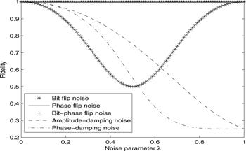
Based on the aforementioned calculation results, we can conclude that the fidelity of the output state is dependent on both the coefficients of the prepared state and the noise parameters under five types of noisy environment. Here we just consider the relationship between the fidelity and noise parameter when the prepared state is determined. Take the measurement result $| {\eta }_{00}^{1}\rangle | {\eta }_{01}^{2}\rangle | {\eta }_{10}^{3}\rangle | 1\rangle $ as an example, assume that the cyclically prepared state is $\tfrac{1}{\sqrt{2}}(| 0\rangle +| 1\rangle )\otimes \tfrac{1}{\sqrt{2}}(| 0\rangle +| 1\rangle )\otimes \tfrac{1}{\sqrt{2}}(| 0\rangle +| 1\rangle )$, $({\alpha }_{j}={\beta }_{j}\,=\tfrac{1}{\sqrt{2}},j=1,2,3)$, we calculate the fidelities in five types of noises and present them in table 3. We further plot the image of the fidelity as the function of noise parameter λ in figure 1.
Figure 1. The plot of the function between fidelity and noise parameter λ. |
Table 3. The fidelities in five types of noisy environment when the cyclically prepared state is $\tfrac{1}{\sqrt{2}}(| 0\rangle +| 1\rangle )\otimes \tfrac{1}{\sqrt{2}}(| 0\rangle \,+| 1\rangle )\otimes \tfrac{1}{\sqrt{2}}(| 0\rangle +| 1\rangle )$. |
| Noise | The fidelity F* |
|---|---|
| Bit-flip | 1 |
| Phase-flip or Bit-phase flip | $\tfrac{{\lambda }^{6}+{\widetilde{\lambda }}^{6}}{{\left(2{\lambda }^{2}-2\lambda +1\right)}^{3}}$ |
| Phase-damping | $\tfrac{4{\widetilde{\lambda }}^{6}+\tfrac{1}{8}{\lambda }^{6}+\tfrac{3}{2}{\lambda }^{2}{\widetilde{\lambda }}^{4}+\tfrac{1}{8}{\lambda }^{4}{\widetilde{\lambda }}^{2}}{{\lambda }^{6}+4{\widetilde{\lambda }}^{6}+6{\lambda }^{2}{\widetilde{\lambda }}^{4}+3{\lambda }^{4}{\widetilde{\lambda }}^{2}}$ |
| Amplitude- damping | $\tfrac{{\lambda }^{6}+{\left(2-\lambda \right)}^{6}+3{\lambda }^{2}{\widetilde{\lambda }}^{4}\,+\,3{\lambda }^{4}{\widetilde{\lambda }}^{2}}{8[{\lambda }^{6}+3{\lambda }^{2}{\widetilde{\lambda }}^{4}+3{\lambda }^{4}{\widetilde{\lambda }}^{2}+{\left({\lambda }^{2}-2\lambda +2\right)}^{3}]}$ |
Obviously, the fidelity is always one under bit-flip noise regardless of the variation of the noise parameter λ. Interestingly, the fidelities are the same under the phase flip and bit-phase flip noises, which first decrease and then increase with the increase of noise parameter λ. When $\lambda =\tfrac{1}{2}$, the fidelities under the phase flip and bit-phase flip noises both reach a minimum value $\tfrac{1}{4}$, which means more information has been lost. While in phase-damping noise, the fidelity also first decreases and then increases with λ changes. In the amplitude-damping noisy environment, the fidelity reduces as the noise parameter λ increases and has a minimum value $\tfrac{1}{8}$. In short, the lower the fidelity, the more information is lost.
6. Conclusions
In this paper, we put forward a protocol for cyclically preparing arbitrary single-qubit states in one direction simultaneously and deterministically. At first, we propose a CCRSP protocol with three senders to prepare three arbitrary single-qubit states by sharing a seven-qubit entangled state. Several simple operations of single-qubit measurement, two-qubit projective measurement and Pauli operations are needed to accomplish the task. One of the unique advantages of our solution is that the senders do not need to employ information splitting and additional unitary operations before making measurements. With the aid of network coding, allowing network nodes to encode and combine the received messages, n-bit CCC can be saved in our protocol. In addition, we consider the case of multiple senders and give a universal CCRSP protocol, which could better meet the requirements of future quantum network communication. Obviously, bidirectional controlled remote preparation is a specific case of the CCRSP with two senders.
As widely known, quantum noise inevitably exists in the communication environment. We also discuss the impact of five types of quantum noises on the proposed CCRSP scheme with three senders, and fidelity is utilized to measure the quality of quantum communication. By calculating and analyzing, we can conclude that the fidelity is dependent on the coefficients of the prepared state and the noise parameters. The higher the fidelity, the better the communication and less information has been lost. Therefore, a quantum communication protocol with resistance to quantum noise will be a more interesting topic in our subsequent research.