Welcome to visit Communications in Theoretical Physics,
Gravitation Theory, Astrophysics and Cosmology

Comprehensive analysis of relativistic embedded class-I exponential compact spheres in f(R, φ) gravity via Karmarkar condition

  • Zoya Asghar , 1 ,
  • Adnan Malik , 2, 3, ,
  • M Farasat Shamir , 1 ,
  • Fatemah Mofarreh , 4
Expand
  • 1 National University of Computer and Emerging Sciences, Lahore Campus, Pakistan
  • 2School of Mathematical Sciences, Zhejiang Normal University, Jinhua, Zhejiang, China
  • 3Department of Mathematics, University of Management and Technology, Sialkot Campus, Pakistan
  • 4 Mathematical Science Department Faculty of Science Princess Nourah bint Abdulrahman University, Riyadh 11546, Saudi Arabia

Author to whom all correspondence should be addressed.

Received date: 2023-03-17

  Revised date: 2023-08-17

  Accepted date: 2023-08-17

  Online published: 2023-09-13

Copyright

© 2023 Institute of Theoretical Physics CAS, Chinese Physical Society and IOP Publishing

Abstract

In this article, we use the prominent Karmarkar condition to investigate some novel features of astronomical objects in the f(R, φ) gravity; R and φ represent the Ricci curvature and the scalar field, respectively. It is worth noting that we classify the exclusive set of modified field equations using the exponential type model of the f(R, φ) theory of gravity f(R, φ) = φ(R + α(e βR − 1)). We show the embedded class-I approach via a static, spherically symmetric spacetime with an anisotropic distribution. To accomplish our objective, we use a particular interpretation of metric potential (grr) that has already been given in the literature and then presume the Karmarkar condition to derive the second metric potential. We employ distinct compact stars to determine the values of unknown parameters emerging in metric potentials. To ensure the viability and consistency of our exponential model, we execute distinct physical evolutions, i.e. the graphical structure of energy density and pressure evolution, mass function, adiabatic index, stability, equilibrium, and energy conditions. Our investigation reveals that the observed anisotropic findings are physically appropriate and have the highest level of precision.

Cite this article

Zoya Asghar , Adnan Malik , M Farasat Shamir , Fatemah Mofarreh . Comprehensive analysis of relativistic embedded class-I exponential compact spheres in f(R, φ) gravity via Karmarkar condition[J]. Communications in Theoretical Physics, 2023 , 75(10) : 105401 . DOI: 10.1088/1572-9494/acf123

1. Introduction

The rapid evolution of the cosmos is one of the most intriguing dimensions of study in astrophysics in recent years. According to astrophysicists, the Universe's energy structure is 20% dark matter (DM), 76% dark energy (DE), and 4% ordinary matter (OM) [14]. Whereas DM pressure is nearly nonexistent compared to the DE's strong negative pressure. Cosmologists believe that dark energy is the primary factor causing the Universe's enigmatic evolution. Although general relativity (GR) offers a basic concept of gravitational notions and produces excellent results in a relativistic theory, it is not sufficient when dealing with difficulties like the unknown DE's exotic nature. These gravitational theories are acknowledged as the modified theories of gravity and the most suitable replacement for GR. Various modified theories available in the literature include f(R), f(R, T), f(R, φ), f(R, G), f(R, φ, X) and f(R, RαβRαβ, φ) gravitational theories [531]. It is interesting to note that astronomers plan to study the collapsing attributes of celestial configurations with the asset of modified gravitational theories. Buchdahl [13] introduced the f(R) gravity, which modifies the Einstein action by utilizing any arbitrary Ricci scalar function. The exponential-type gravity models were introduced by Cognola et al [32] to investigate the physical attributes of astronomical formations. Harko [7] introduced the f(R, T) gravity theory, which is an amalgamation of the curvature or matter. Sharif and Ikram [33] presented f(G, T) gravity and probed the stability attributes. Capozziello and Laurentis [34], who also talked about f(R, φ) gravity, first proposed the scalar field in action. They argued about a unique method for resolving and addressing GR's flaws. The nature of relativistic compact structures in the f(R, φ) gravity was studied by Shamir, and Malik [35]. Various literature has been available related to scalar-tensor theories [3641]. The modified f(R, φ) gravity, which specifies the structure of the inner space, was studied by Malik [42] to determine how charged compact stars behave.
Cosmologists illustrated various theories about the formation of stellar objects. Gravitational forces occurring at the core of compact stars are intensely exothermic. This reaction occurs when the interior pressure of the realistic structure falls to preserve the pressure against the exterior gravitational implosion. Distinct types of intense stars, including white dwarfs, gravastars, neutron stars, black holes, or quark stars, appeared due to the imploding stars. These stars are categorized according to their masses and are an intriguing issue within the background of modified theories. Although the precise nature of these things is yet unclear, one might surmise that they are massive objects with small radii. To explore the exotic nature of such stellar configuration models, we require an accurate outcome to Einstein field equations (EFE), which was first computed by Schwarzschild [43] in 1916. Afterward, Tolman [44] and Oppenheimer [45] provided a detailed review of celestial structures. They claimed that the physical properties of astrophysical configurations demonstrated the interaction between inner pressure and gravitational force, which preserves an equilibrium condition. Baade and Zwicky [46] were among the first researchers to discuss the idea of cosmic star structure. Later, Ruderman [47] investigated the celestial sphere in the source of anisotropic fluid and declared that the density of nuclear elements shows anisotropic behavior at the center. A perfect isotropic fluid was believed to be the basis of stellar systems in the formation of astrophysical structures. These stars are classified as stellar, isotropic, spherically symmetric, and highly heavy objects. But still, some physical elements of compact stars may not be expressed by this isotropic feature. In astronomy, the anisotropic fluid is gaining much attention as a worthy substitute for isotropic matter distribution. Anisotropy is assumed as the fluid due to the combination of distinct types of fluids, magnetic field, viscosity, rotation, etc. Bowers and Liang [48] discussed the notion of non-zero anisotropy in the creation of stars. Furthermore, Ruderman [47] was the first to propose that the celestial structure's high density illustrates the anisotropy at the stellar object's core. Various literature has been presented in the context of anisotropic distribution [4953]. Also, the anisotropic pressures are categorized into radial and transverse distributions.
Astrophysicists used the EFE explanatory method to investigate a four-dimensional manifold family that transforms into Euclidean space for a well-behaved astronomical structure. Nash [54] discovered the first isometric embedding theorem. Later, Gunther [55] provided a modified version of this theorem. Gupta and Sharma [56] utilized the plane metric to obtain the embedded class method. The Karmarkar condition is a differential equation that the embedded classes develop in spherically symmetric spacetime that comprises both the potential components, i.e. grr and gtt. The mentioned condition was introduced by Karmarkar [57] and is defined as R1414R2323 = R1212R3434 + R1224R1334. There is a vast amount of literature on the Karmarkar condition. Maurya et al [58] and Bhar et al [59] examined the response of astrophysical objects in the analysis of GR by using Karmarkar and embedded class-I conditions. Sharif and Saba [60] explored the Karmarkar condition in f(G) gravity along with the anisotropic charged solution, and their results are symmetric and consistent. Naz et al [61] studied the possibility of a unique variety of embedding class-I results of astrophysical objects by utilizing the Karmarkar constraints in the f(R) gravity. Asghar et al [62] probed the different stellar structures in f(R, T) gravity with the help of the Karmarkar condition. Rahaman et al [63] examined the embedding class-I solution for studying the anisotropic structures by implementing the Karmarkar requirement in the f(R, T) gravity. Singh et al [64] apply an embedding approach to explore the graphical features of sphere configurations in f(R, T) gravity. After getting motivated by the prior literature, we further extend the Asghar et al [62] notion in modified f(R, φ) gravity by implementing the Karmarkar condition to examine the physical attributes of various stellar stars. For the present analysis, we consider the exponential f(R, φ) gravity model, i.e. f(R, φ) = φ(R + α(eβR − 1)) [32]. Also, using a precise solution for the metric potential grr [65] that has already been published in the literature, we employ the well-known Karmarkar condition to calculate the second metric potential.
The format of our profile is as follows: in the next part, the modified EFE's, as well as a realistic model of f(R, φ) theory, are explored in the light of the Karmarkar condition. Section 3 is concerned with junction conditions for obtaining constants by contrasting the internal geometry to Schwarzschild's external spacetime. The graphical study is described in section 4, which includes the anisotropic component, stability analysis, Tolman-Oppenheimer-Volkoff equation (TOV), equation of state parameters, mass-radius connection, and surface redshift analysis. We finalized the key findings in the concluding portion.

2. Modified f(R, φ) field equations via Karmarkar condition

The scalar-tensor theories [66] are a fascinating group of extended theories of gravity. This subsection provides an overview of the f(R, φ) theory of gravity and discusses how it applies to static spherically symmetric stellar structures. The following effective action results in a wide range of higher-order scalar-tensor theories [67] as
$\begin{eqnarray}S=\frac{1}{2\kappa }\int {{\rm{d}}}^{4}\sqrt{-g}(f(R,\phi )+w(\phi ){\phi }_{;\xi }{\phi }^{;\xi }+{L}_{m}).\end{eqnarray}$
Here, f(R, φ) is a function that depends on curvature R and scalar field φ. Also, −g illustrates the determinant of gηζ. The EFE's of f(R, φ) are derived by varying the action in equation (1) concerning the metric tensor.
$\begin{eqnarray}\begin{array}{l}{f}_{R}(R,\phi ){R}_{\eta \zeta }-\displaystyle \frac{1}{2}(f(R,\phi )+w(\phi ){\phi }_{;\xi }{\phi }^{;\xi }){g}_{\eta \zeta }\\ \quad +\,w(\phi ){\phi }_{;\eta }{\phi }_{;\zeta }+({g}_{\eta \zeta }\square -{{\rm{\nabla }}}_{\eta }{{\rm{\nabla }}}_{\zeta }){f}_{R}(R,\phi )=8\pi {T}_{\eta \zeta },\end{array}\end{eqnarray}$
where, w is a function of φ, whereas, ≡ ∇ηζ and ∇η indicate the D'Alembertian symbol and covariant derivative, and ${f}_{R}(R,\phi )=\tfrac{{\rm{d}}f(R,\phi )}{{\rm{d}}R}$ respectively. Therefore, the Klein-Gordon equation may be derived by varying the action in equation (1) concerning the scalar field.
$\begin{eqnarray}2w(\phi )\square \phi +w(\phi ){\phi }_{;\xi }{\phi }^{;\xi }-{f}_{\phi },\end{eqnarray}$
where, ${f}_{\phi }(R,\phi )=\tfrac{f(R,\phi )}{{\rm{d}}\phi }$ and ${w}_{\phi }=\tfrac{{\rm{d}}w}{{\rm{d}}\phi }.$ Moreover, the energy-momentum tensor Tηζ is defined as
$\begin{eqnarray}{T}_{\eta \zeta }=(\rho +{p}_{t}){u}_{\eta }{u}_{\zeta }-{p}_{t}{g}_{\eta \zeta }+({p}_{r}-{p}_{t}){{ \mathcal X }}_{\eta }{{ \mathcal X }}_{\zeta }.\end{eqnarray}$
Here, ρ, pr, and pt stand for density and the pressure components, i.e. (radial and tangential). Also, uη and ${{ \mathcal X }}_{\eta }$ are four velocity components, which meet the connection ${u}^{\eta }{u}_{\eta }=-{{ \mathcal X }}^{\eta }{{ \mathcal X }}_{\eta }=1$. Further, we assume a static spherically symmetric spacetime provided by
$\begin{eqnarray}{\rm{d}}{s}^{2}={{\rm{e}}}^{\nu (r)}{\rm{d}}{t}^{2}-{{\rm{e}}}^{\lambda (r)}{\rm{d}}{r}^{2}-{r}^{2}({\rm{d}}{\theta }^{2}+{\sin }^{2}\theta {\rm{d}}{\phi }^{2}).\end{eqnarray}$
Here, ν and λ are only the functions of r. Moreover, to investigate the consistency and equilibrium of the compact system, we examine an exponential model of the f(R, φ) gravity, which assists us in getting a comprehensive performance of the formation of realistic structures. The exponential f(R, φ) gravity model [32] is depicted as
$\begin{eqnarray}f(R,\phi )=\phi (R+\alpha ({{\rm{e}}}^{-\beta R}-1)).\end{eqnarray}$
Here, α and β are unknown parameters and φrχ. We assume w(φ) = w0φm, where m can be any non-zero value. It is worth noting that the consideration of the Klein-Gordon equation (3) is required for the relevant outcomes. Also, the spacetime metric reveals the class of an embedded class-I and whether it fulfilled the prominent Karmarkar condition [57], which is stated as
$\begin{eqnarray}{R}_{1414}{R}_{2323}={R}_{1212}{R}_{3434}+{R}_{1224}{R}_{1334},\end{eqnarray}$
with R2323 ≠ 0. By substituting the Riemann tensor components into equation (7), we get the succeeding differential form
$\begin{eqnarray}{\lambda }^{{\prime} }{\nu }^{{\prime} }-2{\nu }^{{\prime\prime} }-{{\nu }^{{\prime} }}^{2}=\displaystyle \frac{{\lambda }^{{\prime} }{\nu }^{{\prime} }}{1-{{\rm{e}}}^{\lambda }},\end{eqnarray}$
The integration of the above gives the following form of equation
$\begin{eqnarray}{{\rm{e}}}^{\nu }=\left[{\left(A+B\int \sqrt{{{\rm{e}}}^{\lambda }-1}{\rm{d}}r\right)}^{2}\right],\end{eqnarray}$
where, A and B are integrating constants. We presume a specific value of the metric potential grr = eλ(r) [65] to calculate the results of embedded class-I
$\begin{eqnarray}{{\rm{e}}}^{\lambda }=1+\displaystyle \frac{{a}^{2}{r}^{2}}{{\left(1+{{br}}^{2}\right)}^{4}},\end{eqnarray}$
where, a and b can be any non-zero constant parameters. When equation (10) is substituted for equation (9), the metric potential eν has the value
$\begin{eqnarray}{{\rm{e}}}^{\nu }=\left[{\left(A-\displaystyle \frac{{aB}}{2b(1+{{br}}^{2})}\right)}^{2}\right].\end{eqnarray}$
Furthermore, to investigate the implications of our chosen f(R, φ) model, we examined the essential requirements for the metric tensors of static spherically symmetric spacetime, namely eλ(0)=1 and ${\left(({{\rm{e}}}^{\lambda (r)})^{\prime} \right)}_{r=0}=0$. The physical structure of grr ought to be free of singularities, uniform, and monotonically increasing for a realistic f(R, φ) gravity model. Figure 1 shows the physical nature of eλ(r), which increases monotonically and attains its highest value towards the boundary. Hence, using equations (6), (10), and (11), the modified f(R, φ) field equations stated in equation (2) yields
$\begin{eqnarray*}\begin{array}{l}\rho =\frac{1}{2}\left(\frac{4{abB}{{ \mathcal X }}_{2}\left(2{a}^{2}{r}^{2}{\left({{br}}^{2}+1\right)}^{3}-\left({{br}}^{2}-3\right){\left({{br}}^{2}+1\right)}^{6}\right)}{{\left({a}^{2}{r}^{2}+{\left({{br}}^{2}+1\right)}^{4}\right)}^{2}\left(2{Ab}\left({{br}}^{2}+1\right)-{aB}\right)}\right.\\ \quad -\,\frac{2{\left({{br}}^{2}+1\right)}^{3}{{ \mathcal X }}_{3}\left({a}^{2}{r}^{2}\left(3-{{br}}^{2}\right)+2{\left({{br}}^{2}+1\right)}^{5}\right)}{r{\left({a}^{2}{r}^{2}+{\left({{br}}^{2}+1\right)}^{4}\right)}^{2}}\\ \quad -\,\frac{2{{ \mathcal X }}_{4}}{\frac{{a}^{2}{r}^{2}}{{\left({{br}}^{2}+1\right)}\ ^{4}}\ +1}+\frac{\chi {w}_{0}{r}\ ^{\chi -1}\ {\left({r}^{\chi }\right)}^{m}}{\frac{{a}^{2}{r}^{2}}{{\left({{br}}^{2}+1\right)}\ ^{4}}\ +1}+\alpha {r}^{\chi }\\ \quad \left.-\,\alpha {r}^{\chi }{{\rm{e}}}^{-\beta {{ \mathcal X }}_{1}}-{r}^{\chi }{{ \mathcal X }}_{1}\Space{0ex}{2.5ex}{0ex}\right),\end{array}\end{eqnarray*}$
$\begin{eqnarray*}\begin{array}{l}{p}_{r}=\frac{1}{2}\left(\frac{4{\left({{br}}^{2}+1\right)}^{3}{{ \mathcal X }}_{3}\left(2{Ab}\left({a}^{2}\left(2{r}^{2}-2{b}^{2}{r}^{6}\right)+{\left({{br}}^{2}+1\right)}^{6}\right)+{aB}\left({a}^{2}{r}^{2}\left(3{{br}}^{2}-2\right)-{\left({{br}}^{2}+1\right)}^{4}\right)\right)}{r{\left({a}^{2}{r}^{2}+{\left({{br}}^{2}+1\right)}^{4}\right)}^{2}\left(2{Ab}\left({{br}}^{2}+1\right)-{aB}\right)}\right.\\ \quad +\frac{4a{\left({{br}}^{2}+1\right)}^{3}\left(3{{br}}^{2}-1\right){{ \mathcal X }}_{2}\left({a}^{2}B-2{aAb}\left({{br}}^{2}+1\right)+{bB}{\left({{br}}^{2}+1\right)}^{3}\right)}{{\left({a}^{2}{r}^{2}+{\left({{br}}^{2}+1\right)}^{4}\right)}^{2}\left(2{Ab}\left({{br}}^{2}+1\right)-{aB}\right)}\\ \quad +\frac{\chi {w}_{0}{\left({{br}}^{2}+1\right)}^{4}{r}^{\chi -1}{\left({r}^{\chi }\right)}^{m}}{{a}^{2}{r}^{2}+{\left({{br}}^{2}+1\right)}^{4}}\\ \quad \left.+{r}^{\chi }\left(\alpha \left({{\rm{e}}}^{-\beta {{ \mathcal X }}_{1}}-1\right)+{{ \mathcal X }}_{1}\right)\Space{0ex}{2.75ex}{0ex}\right),\end{array}\end{eqnarray*}$
$\begin{eqnarray*}\begin{array}{l}{p}_{t}=\frac{{\left({{br}}^{2}+1\right)}^{3}{{ \mathcal X }}_{3}\left(2{Ab}\left({a}^{2}\left(2{r}^{2}-2{b}^{2}{r}^{6}\right)+{\left({{br}}^{2}+1\right)}^{6}\right)+{aB}\left({a}^{2}\left(4{{br}}^{4}-2{r}^{2}\right)+\left({{br}}^{2}-1\right){\left({{br}}^{2}+1\right)}^{4}\right)\right)}{r{\left({a}^{2}{r}^{2}+{\left({{br}}^{2}+1\right)}^{4}\right)}^{2}\left(2{Ab}\left({{br}}^{2}+1\right)-{aB}\right)}\\ \quad +\frac{a{{ \mathcal X }}_{2}\left(-2{a}^{3}{{Abr}}^{2}\left({{br}}^{2}+1\right)+2{a}^{2}B{\left({{br}}^{2}+1\right)}^{3}+{a}^{4}{{Br}}^{2}+4{aAb}\left({{br}}^{2}-1\right){\left({{br}}^{2}+1\right)}^{4}+2{bB}{\left({{br}}^{2}+1\right)}^{7}\right)}{{\left({a}^{2}{r}^{2}+{\left({{br}}^{2}+1\right)}^{4}\right)}^{2}\left({aB}-2{Ab}\left({{br}}^{2}+1\right)\right)}\\ \quad +\frac{{{ \mathcal X }}_{4}}{\frac{{a}^{2}{r}^{2}}{{\left({{br}}^{2}+1\right)}\ ^{4}}\ +1}+\frac{1}{2}{r}^{\chi }\left(\alpha \left({{\rm{e}}}^{-\beta {{ \mathcal X }}_{1}}-1\right)-\frac{\chi {w}_{0}{\left({r}^{\chi }\right)}^{m}}{\frac{{a}^{2}{r}^{3}}{{\left({{br}}^{2}+1\right)}\ ^{4}}\ +r}\right)+\frac{1}{2}{r}^{\chi }{{ \mathcal X }}_{1}.\end{array}\end{eqnarray*}$
Here,
$\begin{eqnarray*}{{ \mathcal X }}_{1}=\displaystyle \frac{2a\left(-2{a}^{3}{{Abr}}^{2}\left({{br}}^{2}+1\right)-{a}^{2}B\left({{br}}^{2}-3\right){\left({{br}}^{2}+1\right)}^{3}+{a}^{4}{{Br}}^{2}+2{aAb}\left(5{{br}}^{2}-3\right){\left({{br}}^{2}+1\right)}^{4}-2{bB}\left({{br}}^{2}-3\right){\left({{br}}^{2}+1\right)}^{6}\right)}{{\left({a}^{2}{r}^{2}+{\left({{br}}^{2}+1\right)}^{4}\right)}^{2}\left(2{Ab}\left({{br}}^{2}+1\right)-{aB}\right)},\end{eqnarray*}$
$\begin{eqnarray*}{{ \mathcal X }}_{2}=1-\alpha \beta {{\rm{e}}}^{-\beta {{ \mathcal X }}_{1}},\qquad {{ \mathcal X }}_{3}=\frac{\partial {{ \mathcal X }}_{2}}{\partial r},\qquad {{ \mathcal X }}_{4}=\frac{\partial {{ \mathcal X }}_{3}^{2}}{\partial {r}^{2}}.\end{eqnarray*}$
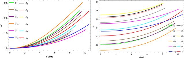
Figure 1. Behavior of metric potential grr and gtt.

3. Junction conditions

Whatever the geometry of the star is, either derived internally or externally, the intrinsic boundary metric remains the same. Thus, ensuring that the elements of the metric tensor irrespective of the coordinate system across the surface of the boundary will remain continuous. No doubt, in GR, the Schwarzschild solutions have been pioneers in guiding us to choose from the various possibilities of the junction conditions while exploring the celestial stars. Now when we come to the case of modified theories of gravity, modified TOV equations with zero pressure and energy density, the solution outside the star can vary from Schwarzschild's solution. However, it is expected that the solutions of the modified TOV equations [44, 45] with energy density and pressure (maybe non-zero) may adjust Schwarzschild's solution with some distinct preference of f(R, φ) gravity model. Perhaps this is the reason that Birkhoff's theorem may not hold in modified gravity [68]. The detailed examination of the issue in f(R, φ) gravity can be an interesting task. Many authors have assumed the Schwarzschild solution for this purpose giving some impressive outcomes [171]. Now to solve the field equations under the restricted boundary essentials at r = R, the pressure pr = 0, the internal metric (5) needs these matching conditions. To resolve the EFE with the limited restriction at r = R, we contrast our inner geometry to the exterior Schwarzschild solution, which is described by
$\begin{eqnarray}\begin{array}{l}{\rm{d}}{s}^{2}=\left(1-\frac{2M}{r}\right){\rm{d}}{t}^{2}-{\left(1-\frac{2M}{r}\right)}^{-1}{\rm{d}}{r}^{2}\\ \quad -{r}^{2}({\rm{d}}{\theta }^{2}+{\sin }^{2}\theta {\rm{d}}{\phi }^{2}),\end{array}\end{eqnarray}$
where, M is the mass of compact sphere. The continuity of metric parameters of equation (5) at r = R emerges in the governing equations:
$\begin{eqnarray}{{g}_{{rr}}}^{+}={{g}_{{rr}}}^{-},\,\,\,\,\,\,\,\,\,\,{{g}_{{tt}}}^{+}={{g}_{{tt}}}^{-},\,\,\,\,\,\,\,\,\,\,\displaystyle \frac{\partial {{g}_{{tt}}}^{+}}{\partial r}=\displaystyle \frac{\partial {{g}_{{tt}}}^{-}}{\partial r}\,.\end{eqnarray}$
In this case, (+) and (−) represent the external and internal structures. We use equations (5), (12), and (13) to calculate the values of the parameters as
$\begin{eqnarray}\begin{array}{rcl}a & = & \displaystyle \frac{{\left(1+{{bR}}^{2}\right)}^{2}}{R}\sqrt{\displaystyle \frac{\tfrac{2M}{R}}{1-\tfrac{2M}{R}}},\\ b & = & \displaystyle \frac{4M-R}{{R}^{2}(9R-20M)},\end{array}\end{eqnarray}$
$\begin{eqnarray}A=\displaystyle \frac{{aB}}{2b(1+{{bR}}^{2})}+\sqrt{1-\displaystyle \frac{2M}{R}},\qquad B=\left(\displaystyle \frac{1}{2R}\right)\sqrt{\displaystyle \frac{2M}{R}}\,.\end{eqnarray}$
Table 1 contains the constants a, b, A and B for the mass and radius of the selected stellar spheres. Furthermore, it is imperative to emphasize that the following constraints should be met for celestial stars to behave properly:

The behavior of ρ, pr and pt should be optimistic, continuous, and maxima in the apex.

The plots of $\tfrac{{\rm{d}}{p}_{r}}{{\rm{d}}r},$ $\tfrac{{\rm{d}}{p}_{t}}{{\rm{d}}r}$ and $\tfrac{{\rm{d}}\rho }{{\rm{d}}r}$ all have to be non-positive.

Each one of the energy parameters should be accomplished.

The equilibrium consistency requirement must be met by all of the forces.

The parameters vr2 and vt2 have to be in the range [0, 1].

Table 1. Unknown parameters of the compact structures.
Star model M (MΘ) R (km) b (km) a (km) B (km) A (km)
4U 1538-52 (S1) 0.87 ± 0.07 [72] 7.866 ± 0.21 −0.000 105 899 0.122 14 0.044 3339 −25.0131
SAX J1808.4-3658 (S2) 0.9 ± 0.3 [72] 7.951 ± 1.0 −0.000 920 891 0.079 3101 0.036 4385 −0.851 084
Her X-1 (S3) 0.85 ± 0.15 [72] 8.1 ± 0.41 −0.000 977 202 0.072 6952 0.034 4393 −0.538 845
LMC X-4 (S4) 1.04 ± 0.09 [72] 8.301 ± 0.2 −0.000 705 186 0.083 8586 0.036 7192 −1.502 07
SMC X-4 (S5) 1.29 ± 0.05 [72] 8.831 ± 0.09 −0.000 366 545 0.093 4356 0.037 2694 −4.137 13
Cen X-3 (S6) 1.49 ± 0.08 [72] 9.178 ± 0.13 −0.000 104 682 0.103 164 0.037 8044 −18.0737
4U 1608-52(S7) 1.74 ± 0.14 [73] 9.3 ± 1.0 0.000 368 416 0.127 851 0.040 0518 7.402 05
PSR J1903 + 327 (S8) 1.667 ± 0.021 [72] 9.48 ± 0.03 0.000 142 764 0.113 994 0.038 346 15.807
Vela X-1 (S9) 1.77 ± 0.08 [72] 9.56 ± 0.08 0.000 306 813 0.122 018 0.038 7589 8.168 31
PSR J1614-2230 (S10) 1.97 ± 0.04 [74] 9.69 ± 0.2 −0.000 739 078 0.145 463 0.040 07 4.317 39
EXO 1785-248 (S11) 1.30 ± 0.2 [74] 10.10 ± 0.44 −0.000 447 232 0.070 8703 0.030 5887 −1.753 21
4U 1820-30 (S12) 1.58 ± 0.06 [75] 10.56 ± 0.10 −0.000 2209 0.080 4744 0.031 5431 −5.144 66

4. Physical analysis of f(R, φ) gravity model

Further, we explore the pictorial behavior of the sphere objects under discussion within the light of the f(R, φ) gravity model. We examine various physical investigations, including density, pressure components, mass component, surface redshift, stability, energy and equilibrium conditions. All features are important in describing the characteristics of compact objects. The free parameter β is chosen for the considered stars in such a way i.e. β = 1 for (S1, S2, S3, S4, S5, S7, S8, S10, S11, S12) and β = 1.5 for (S6, S9).

4.1. Energy density and pressure progression

Here, we examine how the f(R, φ) gravity model affects the graphical representations of the ρ, pr and pt. Figure 2 makes it abundantly evident that all graphs represent optimistic behavior. Also, these graphs reach their peak values at the core and contact the surface at the border, demonstrating that they behave comprehensively.
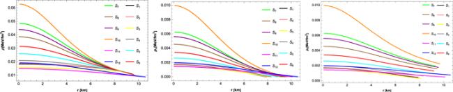
Figure 2. Graphical variations of ρ, pr and pt for α = 0.01, χ = 1 × 10⁷, w0 = 1, m = 1, β = 1 for (S1, S2, S3, S4, S5, S7, S8, S10, S11, S12) and β = 1.5 for (S6, S9).
As part of our discussion, figure 3 displays the graphs for the gradients of ρ, pr and pt. These attributes reflect the maximum compactness characteristic of astrophysical objects.
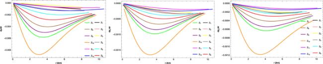
Figure 3. Evolution of $\tfrac{{\rm{d}}\rho }{{\rm{d}}r},$ $\tfrac{{\rm{d}}{p}_{r}}{{\rm{d}}r}$ and $\tfrac{{\rm{d}}{p}_{t}}{{\rm{d}}r}$ for α = 0.01, χ = 1 × 10⁷, w0 = 1, m = 1, β = 1 for (S1, S2, S3, S4, S5, S7, S8, S10, S11, S12) and β = 1.5 for (S6, S9).

4.2. Anisotropy

Here, we explore its graphical response of the anisotropy parameter, defined as Δ = ptpr [76]. Anisotropic factors confirm the validity of stellar objects. Figure 4 shows that the anisotropy component for a given f(R, φ) gravity model demonstrates repulsive behavior when Δ > 0. This suggests that our system behaves appropriately and is reliable.
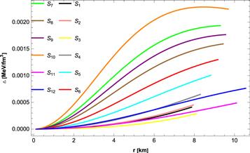
Figure 4. Evolution of anisotropy for α = 0.01, χ = 1 × 10⁷, w0 = 1, m = 1, β = 1 for (S1, S2, S3, S4, S5, S7, S8, S10, S11, S12) and β = 1.5 for (S6, S9).

4.3. Tolman-Oppenheimer-Volkoff equation for f(R, T) gravity

Next, we investigate the equilibrium essential of the f(R, φ) gravity model for the ensuing forces: hydrostatics, anisotropic, and gravitational. To accomplish this, we evaluate the TOV equation [44, 45] assuming as
$\begin{eqnarray}-\frac{{\nu }^{{\prime} }}{r}(\rho +{p}_{r})-\frac{{\rm{d}}{p}_{r}}{{\rm{d}}r}+\frac{2}{r}({p}_{t}-{p}_{r})=0.\end{eqnarray}$
Here,

${{ \mathcal F }}_{a}=\tfrac{2}{r}{\rm{\Delta }}$ symbolize anisotropic force,

${{ \mathcal F }}_{h}=-\tfrac{{\rm{d}}{p}_{r}}{{\rm{d}}r}$ represents hydrostatic force,

${{ \mathcal F }}_{g}=-\tfrac{{\nu }^{{\prime} }}{r}(\rho +{p}_{r})$ is gravitational force.

The total sum of the four forces listed above should equal zero for a realistic model of f(R, φ) gravity. It suggests that all of these forces for an equilibrium scenario cancel out each other's effects and preserve the balanced condition, i.e.
$\begin{eqnarray}{{ \mathcal F }}_{a}+{{ \mathcal F }}_{h}+{{ \mathcal F }}_{g}=0.\end{eqnarray}$
The right panel of figure 5 makes it quite explicit that all forces are fulfilled by the appropriate stability criteria.
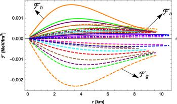
Figure 5. Behavior of ${{ \mathcal F }}_{h}$, ${{ \mathcal F }}_{g}$ and ${{ \mathcal F }}_{a}$ for α = 0.01, χ = 1 × 10⁷, w0 = 1, m = 1, β = 1 for (S1, S2, S3, S4, S5, S7, S8, S10, S11, S12) and β = 1.5 for (S6, S9).

4.4. Energy conditions

Energy conditions play a major contribution in confirming the validity of compact structures. The following factors comprise the well-known energy conditions: There are four categories of energy: dominant energy conditions (DEC), null energy conditions (NEC), weak energy conditions (WEC), and strong energy conditions $(\mathrm{SEC})$, defined as
$\begin{eqnarray*}\begin{array}{l}\mathrm{DEC}:\rho -{p}_{r}\gt 0,\rho -{p}_{t}\gt 0,\\ \quad \mathrm{NEC}:\rho +{p}_{r}\geqslant 0,\rho +{p}_{t}\geqslant 0,\end{array}\end{eqnarray*}$
$\begin{eqnarray*}\begin{array}{l}\mathrm{WEC}:\rho \geqslant 0,\rho +{p}_{r}\geqslant 0,\rho +{p}_{t}\geqslant 0,\\ \quad \mathrm{SEC}:\rho +{p}_{r}\geqslant 0,\rho +{p}_{t}\geqslant 0,\rho +{p}_{r}+2{p}_{t}\geqslant 0.\end{array}\end{eqnarray*}$
Figure 6 illustrates that all attributes are fully served for the investigated exponential f(R, φ) gravity model.
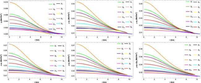
Figure 6. Evolution of energy bonds for α = 0.01, χ = 1 × 10⁷, w0 = 1, m = 1, β = 1 for (S1, S2, S3, S4, S5, S7, S8, S10, S11, S12) and β = 1.5 for (S6, S9).

4.5. Equation of state (EoS) factors

The EoS is now computed for both pressure components. It is a dimensionless quantity that helps to represent the state of matter under certain limitations. The EoS factors are determined as the two ratios i.e. $\tfrac{{pr}}{\rho }$, and $\tfrac{{pt}}{\rho }$. These parameters wr and wt are illustrated as
$\begin{eqnarray}{w}_{r}=\displaystyle \frac{{p}_{r}}{\rho },\,\,\,\,\,\,\,\,{w}_{t}=\displaystyle \frac{{p}_{t}}{\rho }.\end{eqnarray}$
The condition 0 < wr, wt < 1 and we are satisfied by the physical demonstration of wr and wt given in figure 7. As a result, we may conclude that the graphical nature of EoS is appropriate for selected f(R, φ) gravity model.
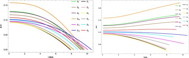
Figure 7. Evolution of wr and wt for α = 0.01, χ = 1 × 10⁷, w0 = 1, m = 1, β = 1 for (S1, S2, S3, S4, S5, S7, S8, S10, S11, S12) and β = 1.5 for (S6, S9).

4.6. Mass-radius function, compactness parameter and surface redshift progression

The mass component ${ \mathcal M }(r),$ compactness parameter ${ \mathcal U }(r),$ and surface redshift element ${ \mathcal Z }{\rm{s}}$ are thought to be essential properties for stellar object evaluation. All of these fundamental features are linked to each other. Also, these anisotropic celestial objects can not be excessively dense in any graphically realistic scenario. Buchdahl [77] determined the highest admissible mass-radius relation for the perfect fluid, which is $\tfrac{2M}{R}\lt \tfrac{8}{9}$. Mak and Harko [78] have presented a modified equation for this mass-to-radius ratio. The mass distribution [65] of astrophysical objects is obtained by comparing the potentials i.e. ${g}_{{rr}}^{-}$ = ${g}_{{rr}}^{+}$ and the final value is
$\begin{eqnarray}{ \mathcal M }(r)=\displaystyle \frac{{a}^{2}{r}^{3}}{2({\left(1+{{br}}^{2}\right)}^{4}+{a}^{2}{r}^{2})}.\end{eqnarray}$
The evolution of the mass distribution demonstrates that mass is constant at the core, i.e. ${ \mathcal M }(r)\to 0$. Also, the mathematical version of the compactness metric ${ \mathcal U }(r)$ is provided as [79]
$\begin{eqnarray}{ \mathcal U }(r)=\displaystyle \frac{2{ \mathcal M }(r)}{r}=\displaystyle \frac{{a}^{2}{r}^{2}}{[{\left(1+{{br}}^{2}\right)}^{2}+{a}^{2}{r}^{2}]}.\end{eqnarray}$
The surface redshift function ${ \mathcal Z }{\rm{s}}$ is described as
$\begin{eqnarray}{{ \mathcal Z }}_{s}=\displaystyle \frac{1}{\sqrt{1-2\nu }}-1.\end{eqnarray}$
Figure 8 shows a graphical representation of the mass function, compactness parameter, and surface redshift. The plots of these factors show monotonically rising behavior. These graphs confirm the consistent nature of the realistic structures.
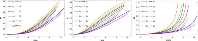
Figure 8. Behavior of ${ \mathcal M }(r),{ \mathcal U }(r),$ and ${ \mathcal Z }{\rm{s}}$ for α = 0.01, χ = 1 × 10⁷, w0 = 1, m = 1, β = 1 for (S1, S2, S3, S4, S5, S7, S8, S10, S11, S12) and β = 1.5 for (S6, S9).

4.7. Stability analysis

The stability analysis in the f(R, φ) gravity is discussed in this section. The causality requirement is essential in the topic of stellar spheres. When the f(R, φ) model shows an inner configuration, the sound velocity of the pressure has to be smaller than the speed of the light. The causality element of pressure waves emerges in radial and transverse dimensions in anisotropic systems. All elements should be constrained to the velocity of context to produce an accurate f(R, φ) framework. The following phrase serves as the basis for the stability condition.
$\begin{eqnarray}{v}_{r}^{2}=\frac{{\rm{d}}{p}_{r}}{{\rm{d}}\rho },\,\,\,\,\,\,\,\,{{v}_{t}}^{2}=\frac{{\rm{d}}{p}_{t}}{{\rm{d}}\rho },\end{eqnarray}$
where, ${{v}_{r}}^{2}$ and ${{v}_{t}}^{2}$ represent the radial and transverse sound velocity. For a physically stable astronomical formation, these sound velocities must fall within the region [0, 1]. To investigate the consistency of the f(R, φ) model, we employ the Herrera technique [80] i.e. $0\leqslant {v}_{r}^{2},{v}_{t}^{2}\leqslant 1$. We also evaluated the Andreasson requirement [81] to guarantee that our suggested model behaves consistently. It is crucial to note that the f(R, φ) model under consideration is entirely static, as shown in figure 9.
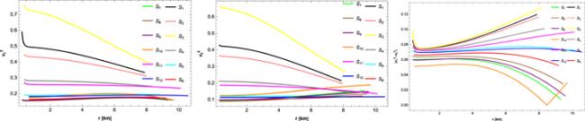
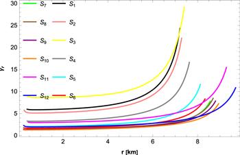
Figure 9. Variations of vr2, vt2 and $| {v}_{t}^{2}-{v}_{r}^{2}| $ for α = 0.01, χ = 1 × 10⁷, w0 = 1, m = 1, β = 1 for (S1, S2, S3, S4, S5, S7, S8, S10, S11, S12) and β = 1.5 for (S6, S9).

4.8. Adiabatic index

We also investigate the stiffness of EoS by examining the adiabatic factor. The adiabatic element value should be higher than $\tfrac{4}{3}$ for a steady structure. The adiabatic parameter proportion is denoted as
$\begin{eqnarray}\gamma =\frac{\rho +{p}_{r}}{{p}_{r}}\left(\frac{{\rm{d}}{p}_{r}}{{\rm{d}}\rho }\right)=\frac{\rho +{p}_{r}}{{p}_{r}}{{v}_{r}}^{2}.\end{eqnarray}$
Our selected exponential f(R, φ) gravity model, as described in figure 10, demonstrates the stable nature of stellar formations. The stability of the model, taking into account the relativistic adiabatic index, requires further analysis due to potential instabilities arising from relativistic corrections to the adiabatic index, denoted as γ [82, 83]. To address this issue, a more rigorous condition was proposed in [84], which introduces the concept of a critical value, γcrit, for the adiabatic index. This critical value depends on the amplitude of the Lagrangian displacement from equilibrium and the compactness factor ${ \mathcal U }(r)\equiv \tfrac{M}{R}$. The amplitude of the Lagrangian displacement is characterized by the parameter ζ. A specific form of this parameter allows for the expression of the critical relativistic adiabatic index.
$\begin{eqnarray}{\gamma }_{\mathrm{crit}}=\frac{4}{3}+\frac{19}{21}{ \mathcal U }(r),\end{eqnarray}$
The stability condition for the model is expressed as γγcrit , as shown in table 2. Notably, the condition γγcrit is consistently met in all cases. Thus, we can confidently assert that the current toy model remains stable when subjected to local radial perturbations induced by relativistic corrections.
Figure 10. Behavior of γ for α = 0.01, χ = 1 × 10⁷, w0 = 1, m = 1, β = 1 for (S1, S2, S3, S4, S5, S7, S8, S10, S11, S12) and β = 1.5 for (S6, S9).
Table 2. The numerical values of adiabatic index d critical adiabatic index for the different compact structures.
Star model M (MΘ) R (km) γ γcrit
4U 1538-52 (S1) 0.87 ± 0.07 [72] 7.866 ± 0.21 336.275 1.553 39
SAX J1808.4-3658 (S2) 0.9 ± 0.3 [72] 7.951 ± 1.0 4909.81 1.485 22
Her X-1 (S3) 0.85 ± 0.15 [72] 8.1 ± 0.41 8521.44 1.474 15
LMC X-4 (S4) 1.04 ± 0.09 [72] 8.301 ± 0.2 1281.51 1.501 45
SMC X-4 (S5) 1.29 ± 0.05 [72] 8.831 ± 0.09 592.332 1.529 35
Cen X-3 (S6) 1.49 ± 0.08 [72] 9.178 ± 0.13 468.623 1.551 18
4U 1608-52 (S7) 1.74 ± 0.14 [73] 9.3 ± 1.0 423.614 1.584 39
PSR J1903 + 327 (S8) 1.667 ± 0.021 [72] 9.48 ± 0.03 440.685 1.570 34
Vela X-1 (S9) 1.77 ± 0.08 [72] 9.56 ± 0.08 446.48 1.581 77
PSR J1614-2230 (S10) 1.97 ± 0.04 [74] 9.69 ± 0.2 513.936 1.606 14
EXO 1785-248 (S11) 1.30 ± 0.2 [74] 10.10 ± 0.44 1539.25 1.506 05
4U 1820-30 (S12) 1.58 ± 0.06 [75] 10.56 ± 0.10 1763.81 1.5341

4.9. Comparison

Shamir and Malik [85] investigated the behavior of stellar structures in f(R, φ) theory of gravity by using three stars namely Her X-1, SAX J 1808.4-3658, and 4U 1820-30. In our recent work, we have investigated the behavior of stars for twelve different stars, which is more comprehensive analysis than [85]. Malik [86] investigated the behavior of charged compact stars in the modified f(R, φ) theory of gravity, by taking four stars like Her X-I, Cen X-III, EXO 1785-248 and LMC X-IV. In our current analysis, we investigated the nature of stellar structures by using the Karmarkar conditions for twelve stars, which makes our work more generalized and comprehensive than the previous investigation.

5. Conclusion

Different modified theories are considered essential features in physics and astronomy to explore the intricate nature of realistic configurations. In these modified frameworks, f(R, φ) gravity attracts the most attention among scientists due to its special combination of curvature and scalar field. Furthermore, f(R, φ) gravity exhibited several outstanding discoveries in the domains of cosmology, thermodynamics, and astrophysics of stellar objects. Further, in this work, we studied the optimal outcomes of EFE in f(R, φ) gravity to precisely study the dynamics of stellar stars with anisotropic fluid sources. To accomplish this, we employ the Karmarkar condition, which simplifies the solution-generating technique to a specific potential by relating gtt with grr. Moreover, we explore the precise formulation for the potential eλ [65], i.e. ${{\rm{e}}}^{\lambda }=1+\tfrac{{a}^{2}{r}^{2}}{{\left(1+{{br}}^{2}\right)}^{4}}$ and extract other potential using the Karmarkar condition, denoted as ${{\rm{e}}}^{\nu }={\left[A-\tfrac{{aB}}{2b(1+{{br}}^{2})}\right]}^{2}$. Here A, B, a and b represent arbitrary unknowns. Furthermore, we use junction conditions to compute the values of unknown factors by contrasting the internal sphere (5) with the Schwarzschild outer geometry (12). To evaluate the stability of our derived solutions, we investigate the graphical behaviors of distinct stellar objects. The goal is to generate a family of embedding class-I solutions to the f(R, φ) theory in the existence of an anisotropic source. The outstanding results are mentioned below:

The physical structure of both potentials in figure 1 reveals that gtt and grr are singularity-free, optimistic, and fulfill the needs, i.e. ${{\rm{e}}}^{\nu (r=0)}={\left[A-\tfrac{{aB}}{2b}\right]}^{2}$ and eλ(r=0) = 1. The response of both metric potentials reveals successful outcomes, as their graphs rise monotonically and achieve maximum levels at the border.

The consistency of ρ, pr and pt for the model under consideration is shown in figure 2. The behavior of these graphs reaches its apex in the core and then declines towards the border.

Figure 3 illustrates the gradient of ρ, pr and pt. These graphs provide non-positive depictions, confirming that our findings are reliable.

Figure 4 demonstrates that Δ > 0, indicating that anisotropic factor is repulsive in nature. This observation confirms the occurrence of astrophysical stars.

All of the forces ${{ \mathcal F }}_{h}$, ${{ \mathcal F }}_{g}$ and ${{ \mathcal F }}_{a}$ are steady and display equilibrium manners, as seen in figure 5.

Figure 6 represents the energy condition for the selected f(R, φ) model. Also, it is worth mentioning that our selected model confirms all of the relevant requirements.

It is clear from figure 7 that the composition of EoS ratios is uniform.

Figure 8 clearly shows the monotonically increasing nature of the mass function, compactness parameter, and surface redshift.

The sound velocity components vr2 and vt2 exist among [0, 1] for the exponential f(R, φ) model. Figure 9 shows that the causality conditions are appropriate for the proposed celestial configuration.

The satisfactory nature of the adiabatic parameter can be noticed in figure 10.

Thus, our research revealed a consistent behavior for all required conditions and well-fitting behavior in the presence of a realistic structure. Also, it is worth saying that our obtained consequences are identical to the conclusions investigated by Asghar et al [62] in the f(R, T) gravity scenario.

Adnan Malik acknowledges the Grant No. YS304023912 to support his Postdoctoral Fellowship at Zhejiang Normal University, China. The author, Fatemah Mofarreh, expresses her gratitude to Princess Nourah bint Abdulrahman University Researchers Supporting Project number (PNURSP2023R27), Princess Nourah bint Abdulrahman University, Riyadh, Saudi Arabia.

1
Astashenok A V Capozziello S Odintsov S D 2013 Further stable neutron star models from f(R) gravity J. Cosmol. Astropart. Phys. 12 040

DOI

2
Eisenstein D J et al 2005 Detection of the baryon acoustic peak in the large-scale correlation function of SDSS luminous red galaxies Astrophys. J. 633 560

DOI

3
Riess A G et al 2004 Type Ia supernova discoveries at z > 1 from the Hubble space telescope: evidence for past deceleration and constraints on dark energy evolution Astrophys. J. 607 665

DOI

4
Spergel D N et al 2007 Three-year Wilkinson microwave anisotropy probe (WMAP) observations: implications for cosmology Astrophys. J., Suppl. Ser. 170 377

DOI

5
Shamir M F Ahmad M 2017 Some exact solutions in f(G, T) gravity via Noether symmetries Mod. Phys. Lett. A 32 1750086

DOI

6
Li B Sotiriou T P Barrow J B 2011 f(T) gravity and local Lorentz invariance Phys. Rev. D 83 064035

DOI

7
Harko B 2011 f(R, T) gravity Phys. Rev. D 84 024020

DOI

8
Capozziello S De Laurentis M Odintsov S D Stabile A 2011 Hydrostatic equilibrium and stellar structure in f(R) gravity Phys. Rev. D 83 064004

DOI

9
Nojiri S Odintsov S D 2011 Unified cosmic history in modified gravity: from f(R) theory to Lorentz non-invariant models Phys. Rep. 505 59

DOI

10
Nojiri S Odintsov S D 2006 Modified f(R) gravity consistent with realistic cosmology: From a matter dominated epoch to a dark energy universe Phys. Rev. D 74 86005

DOI

11
Nojiri S Odintsov S D Oikonomou V K 2017 Modified gravity theories on a nutshell: Inflation, bounce and late-time evolution Phys. Rep. 692 1

DOI

12
Sharif M Ikram A 2016 Warm inflation in f(G) theory of gravity JETP 123 40

DOI

13
Buchdahl H A 1970 Non-linear Lagrangians and cosmological theory Mon. Notices Royal Ast. Soc. 150 1

DOI

14
Starobinsky A A 2007 Disappearing cosmological constant in f(R) gravity JETP Lett. 86 157

DOI

15
Bhar P Pradhan S Malik A Sahoo P K 2023 Physical characteristics and maximum allowable mass of hybrid star in the context of f(Q) gravity Eur. Phys. J. C 83 646

DOI

16
Malik A 2023 Comprehensive study of cylindrical Levi-Civita and cosmic string solutions in Rastall theory of gravity Chin. J. Phys. 84 357

DOI

17
Malik A Naz T Qadeer A Shamir M F Yousaf Z 2023 Investigation of traversable wormhole solutions in modified f(R) gravity with scalar potential Eur. Phys. J. C 83 522

DOI

18
Malik A Tariq A Mardan S A Noureen I 2023 Singularity-free anisotropic strange quintessence stars in f(R, φ, X) theory of gravity Eur. Phys. J. Plus 138 418

DOI

19
Shamir M F Malik A 2019 Investigating f(R, φ) cosmology with equation of state Can. J. Phys. 97 752 760

DOI

20
Malik A Ahmad S Ahmad S 2020 Energy bounds in f(R, φ) gravity with anisotropic backgrounds New Astron. 79 101392

DOI

21
Malik A Shamir M F Hussain I 2020 Noether symmetries of LRS Bianchi type-I spacetime in f(R, φ, X) gravity Int. J. Geom. Methods Mod. Phys. 17 2050163

DOI

22
Malik A Mofarreh F Zia A Ali A 2022 Traversable wormhole solutions in the f(R) theories of gravity under the Karmarkar condition Chinese Phys. C 46 095104

DOI

23
Malik A Nafess A Ali A Naeem M 2022 A study of cylindrically symmetric solutions in f(R, φ, X) theory of gravity Eur. Phys. J. C 82 166

DOI

24
Malik A Ashraf A Naqvi U Zhang Z 2022 Anisotropic spheres via embedding approach in f(R) gravity Int. J. Geom. Methods Mod. Phys. 19 2250073

DOI

25
Malik A 2021 A study of Levi-Civita's cylindrical solutions in f(R, φ) gravity Eur. Phys. J. Plus 136 1146

26
Malik A Nafees A 2021 Existence of static wormhole solutions using f(R, φ, X) theory of gravity New Astron. 89 101632

DOI

27
Malik A Ahmad M Mahmood S 2021 Some dark energy cosmological models in f(R, φ) gravity New Astron. 89 101631

DOI

28
Shamir M F Malik A Mustafa G 2021 Wormhole solutions in modified f(R, φ, X) gravity Int. J. Mod. Phys. A 36 2150021

DOI

29
Shamir M F Malik A 2021 Bardeen compact stars in modified f(R) gravity Chin. J. Phys. 69 312 321

DOI

30
Shamir M F Asghar Z Malik A 2022 Realivistic Krori-Barua compact stars in f(R, T) gravity Fortschr. Phys. 70 2200134

31
Malik A Asghar Z Shamir M F 2023 Krori-Barua Bardeen compact stars in f(R, T) gravity New Astron. 104 102071

DOI

32
Cognola G et al 2008 Class of viable modified f(R) gravities describing inflation and the onset of accelerated expansion Phys. Rev. D 77 046009

DOI

33
Sharif M Ikram A 2016 Energy conditions in f(G, T) gravity Eur. Phys. J. C 76 640

DOI

34
Capozziello S Laurentis M D 2011 Extended theories of gravity Phys. Rep. 509 167

DOI

35
Shamir M F Malik A 2019 Behavior of anisotropic compact stars in f(R, φ) gravity Commun. Theor. Phys. 71 599

DOI

36
Zubair M Kousar F 2016 Cosmological reconstruction and energy bounds in f(R, RαβRαβ, φ) gravity Eur. Phys. J. C 76 254

DOI

37
Waheed S Zubair M Shafiq I Durrani L 2022 Tsallis HDE-based reconstruction via correspondence scheme in a generalized torsion scalar theory Eur. Phys. J. Plus 137 1108

DOI

38
Zubair M Kousar F Bahamonde S 2016 Thermodynamics in f(R, RαβRαβ, φ) theory of gravity Phys. Dark Univ. 14 116

DOI

39
Zubair M Kousar F Bahamonde S 2018 Static spherically symmetric wormholes in generalized f(R, φ) gravity Eur. Phys. J. Plus 133 523

40
Zubair M Kousar F Waheed S 2019 Dynamics of scalar potentials in theory of gravity Can. J. Phys. 97 880894

DOI

41
Zubair M Kousar F Saleem R 2022 Phantom evolving wormhole solutions in scalar-tensor theories Chin. J. Phys. 65 355

DOI

42
Malik A 2022 Analysis of charged compact stars in modified f(R, φ) theory of gravity New Astron. 93 101765

DOI

43
Schwarzschild K 1916 On the gravitational field of a mass point according to einstein's theory Sit. Dts. Aka. Wis. Math. Phys. Ber. 24 424

44
Tolman R C 1939 Static solutions of Einstein's field equations for spheres of fluid Phys. Rev. 55 364

DOI

45
Oppenheimer J R Volkoff G M 1939 On massive neutron cores Phys. Rev. 55 374

DOI

46
Baade W Zwicky F 1934 Phys. Rev. 46 76

DOI

47
Ruderman R 1972 Pulsars: structure and dynamics Annu. Rev. Astron. Astrophys. 10 427

DOI

48
Bowers R L Liang E P T 1974 Anisotropic spheres in general relativity Astrophys. J. 188 657

DOI

49
Herrera L Santos N O 1997 Local anisotropy in self-gravitating systems Phys. Rep. 286 53

DOI

50
Mak M K Harko T 2003 Anisotropic stars in general relativity Pro. R. Soc. A 459 393

DOI

51
Maurya S K Gupta Y K 2013 Charged fluid to anisotropic fluid distribution in general relativity Astrophys. Space Sci. 344 243

DOI

52
Bhar P 2015 Singularity-free anisotropic strange quintessence star Astrophys. Space Sci. 356 309

DOI

53
Bhar P Maurya S K Gupta Y K Manna T 2016 Modelling of anisotropic compact stars of embedding class one Eur. Phys. J. A 52 312

DOI

54
Nash J 1956 The imbedding problem for Riemannian manifolds Ann. Math. 63 20

DOI

55
Günther M 1989 Zum Einbettungssatz von J. Nash Math. Nachr. 144 165

DOI

56
Gupta Y K Sharma J R 1996 Non-static non-conformally flat fluid plates of embedding class one Gen. Relat. Gravit. 28 1447

DOI

57
Karmarkar K R 1948 Gravitational metrics of spherical symmetry and class one Proc. Indian National Sci. Acad. 27 56

DOI

58
Maurya S K Gupta Y K Ray S Deb D 2016 Generalised model for anisotropic compact stars Eur. Phys. J. C 76 693

DOI

59
Bhar P 2017 Modelling a new class of anisotropic compact stars satisfying the karmakar's condition Eur. Phys. J. Plus 132 274

60
Sharif M Saba S 2020 Embedding class-1 anisotropic solution in f(G) gravity Chin. J. Phys. 64 374 389

DOI

61
Naz T Usman A Shamir M F 2021 Embedded class-I solution of compact stars in f(R) gravity with Karmarkar condition Ann. Phys. 429 168491

DOI

62
Asghar Z Shamir M F Usman A Malik A 2023 Study of embedded class-I fluid spheres in f(R, T) gravity with Karmarkar condition Chin. J. Phys. 83 427

DOI

63
Rahaman M Singh K N Errehymy A Rahaman F 2020 Anisotropic Karmarkar stars in f(R, T) gravity Eur. Phys. J. C 80 272

DOI

64
Singh K N Errehymy A Rahaman F Daoud M 2020 Exploring physical properties of compact stars in f(R, T) gravity: an embedding approach Chin. Phys. C 44 105106

DOI

65
Bhar P Singh K N Manna T 2017 A new class of relativistic model of compact stars of embedding class I Int. J. Mod. Phys. D 26 1750090

DOI

66
Stabile A Capozziello S 2013 Galaxy rotation curves in f(R, φ) gravity Phys. Rev. D 87 064002

DOI

67
Lambiase G Sakellariadou M Stabile A Stabile A 2015 Astrophysical constraints on extended gravity models J. Cosmol. Astropart. Phys. JCAP07(2015)003

68
Faraoni V 2010 Jebsen-Birkhoff theorem in alternative gravity Phys. Rev. D 81 044002

DOI

69
Cooney A Deo S D Psaltis D 2010 Neutron stars in f(R) gravity with perturbative constraints Phys. Rev. D 82 064033

DOI

70
Ganguly A Gannouji R Goswami R Ray S 2014 Neutron stars in the Starobinsky model Phys. Rev. D 89 064019

DOI

71
Momeni D Myrzakulov R 2015 Tolman-Oppenheimer-Volkoff equations in modified Gauss-Bonnet gravity Int. J. Geom. Methods Mod. Phys. 12 1550014

DOI

72
Gangopadhyay T Ray S Li X-D Dey J Dey M 2013 Strange star equation of state fits the refined mass measurement of 12 pulsars and predicts their radii Mon. Notices Royal Astron. Soc. 431 3216 3221

DOI

73
Güver T Wroblewski P Camarota L Özel F 2010 The mass and radius of the neutron star in 4U1820 − 30 Astrophys. J. 719 1807

DOI

74
Rawls M L et al 2011 Refined neutron star mass determinations for six eclipsing x-ray pulsar binaries Astrophys. J. 25 730

DOI

75
Güver T Özel F Cabrera-Lavers A Wroblewski P 2010 The distance, mass, and radius of the neutron star in 4U1608 − 52 Astrophys. J. 712 964

DOI

76
Bohmer C G Harko T 2006 Bounds on the basic physical parameters for anisotropic compact general relativistic objects Class. Quantum Grav. 23 6479

DOI

77
Buchdahl H A 1959 General relativistic fluid spheres Phys. Rev. 116 1027 1034

DOI

78
Mak M K Harko T 2003 Anisotropic stars in general relativity Proc. R. Soc. Lond. A 459 393 408

DOI

79
Gokhroo M K Mehra A L 1994 Anisotropic spheres with variable energy density in general relativity Gen. Rel. Grav. 26 75

DOI

80
Herrera L 1992 Cracking of self-gravitating compact objects Phys. Lett. A 165 206

DOI

81
Abreu H Hernandez H Nunez L A 2007 Sound speeds, cracking and the stability of self-gravitating anisotropic compact objects Class Quantum Grav. 24 4631

DOI

82
Chandrasekhar S 1964 The equilibrium and the stability of the Darwin ellipsoids Astrophys. J. 140 417

DOI

83
Chandrasekhar S 1964 Dynamical instability of gaseous masses approaching the Schwarzschild limit in general relativity Phys. Rev. Lett. 12 1143

DOI

84
Moustakidis Ch C 2017, The stability of relativistic stars and the role of the adiabatic index Gen. Relativ. Gravit. 49 68

DOI

85
Shamir M F Malik A 2019 Behavior of anisotropic compact stars in f(R, φ) gravity Commun. Theor. Phys. 71 599

DOI

86
Malik A 2022 Analysis of charged compact stars in modified f(R, φ) theory of gravity New Astron. 93 101765

DOI

Outlines

/