


1. Introduction
A dusty plasma is a unique type of plasma that consists of three distinct components: electrons, ions, and charged dust particles. These dust particles are typically found within a size range of nanometers to several hundreds of micrometers [1, 2]. Dusty plasma, also known as complex plasma, has been the subject of extensive research over the past decades [3–5]. Dusty plasma is present in a wide range of cosmic environments [3, 6–8], including the solar system [6], planetary rings [3, 7], interstellar clouds, circumstellar clouds and various space environments [8]. Understanding the properties and behavior of dusty plasmas is crucial for our understanding of many natural phenomena in space.
There are significant differences between dusty plasma and ion-electron plasma due to the relatively large mass of dust particles [9–11] compared to electrons and ions. One of the obvious differences of the dusty plasma is that the influence of gravity on a dust particle cannot be ignored, particularly on Earth. What is more important is that dusty plasma exhibits complex behavior, including dust acoustic waves [4], dust ion acoustic waves [12], and others [5, 13–17]. These unique properties make dusty plasma an intriguing subject for research in astrophysics, space science, and plasma physics.
Over the past few years, researchers have studied a binary dusty plasma that contains two types of microparticles of different sizes [18, 19]. This binary dusty plasma can either be mixed [20–22] or form a phase-separated system [23–26]. The separation may be caused by spinodal decomposition [25] or an imbalance of external forces [26]. In the latter case, an interface emerges between the separated phases.
As is widely recognized, the Rayleigh-Taylor (RT) instability is a hydrodynamic instability that occurs at the interface between two fluids of different densities when the lighter fluid is accelerated to move into the denser fluid due to an external force [27–29]. This instability is a result of the growth of small perturbations or waves that occur at the interface, causing the fluids to mix and form complex patterns. The RT instability has significant applications in various scientific and engineering fields [30–36], including astrophysics [37], plasma physics [38–41], and others [42–46]. Understanding the RT instability is essential for predicting and controlling the behavior of fluids in these applications. Furthermore, there have been many studies on the RT instability in dusty plasmas [27, 28, 47–49]. For instance, the stability of stratified dust clouds suspended in anode plasma was analyzed, and the RT instability was detected [28]. Additionally, the RT instability finds broad applications in inertial confinement fusion [50, 51], laboratory plasma [52, 53], as well as astrophysical settings like crab nebulae [54] and supernova remnants [55].
Research on RT instability in dusty plasmas has been conducted [56], and while recent studies have investigated this phenomenon, the effects of external magnetic and electric fields on RT instability are still unclear. The present paper aims to study the influence of the magnetic field on RT instability and has found that the charge-mass ratio of the charged particles in the plasma plays a significant role in RT instability and its growth rate. It is worth noting that the larger the charge-mass ratio of the charged particles, the greater the effect of the magnetic field in suppressing the RT instability. Thus, the external magnetic field's ability to suppress the RT instability in ion-electron plasma is much stronger than in dusty plasma. In addition, it has been discovered that in a dusty plasma, the RT instability and its growth rate are influenced not only by region parameters (such as the external magnetic field, the length and gradient of the region) and dust particle parameters (such as dust particle number density, mass, and charge), but also by electron and ion parameters, including their number densities and temperatures.
2. Theoretical model
2.1. RT instability in a dusty plasma
We will study two typical charged fluids. One is the dusty plasma, the other is ion-electron plasma. Following, we first study RT instability in a dusty plasma, which is composed of dust particles, free electrons, and free ions.
Dusty plasma has been found in space plasma, as well as in the laboratory on earth [57–61]. However, it is difficult to form three-dimensional dusty plasma lattice in the laboratory on Earth because of the asymmetric gravity acting on dust particles. Recently, three-dimensional dusty plasma lattices have been achieved under micro-gravity conditions [24] in the Russian-German PK-3 Plus Laboratory aboard the International Space Station (ISS). Furthermore, an interface emerges between two separated phases [18, 19].
To investigate the RT instability at an interface in a dusty plasma, we make the assumption that both electrons and ions can be treated as light fluids that follow the Boltzmann distribution, ${n}_{e}={n}_{e0}\exp \left(\tfrac{e\phi }{{k}_{{\rm{B}}}{T}_{e}}\right)$, ${n}_{i}={n}_{i0}\exp \left(-\tfrac{e\phi }{{k}_{{\rm{B}}}{T}_{i}}\right)$, where ne, ni are the electron number density and ion number density, Te, Ti are the temperatures of electrons and ions, φ is electrostatic potential and kB is Boltzmann constant.
To describe this type of dusty plasma, we utilize the generalized hydrodynamic model, which takes into account the forces produced by the pressure gradient as well as those produced by the electric and magnetic fields acting on the dust particles. The resulting momentum equation for a dusty plasma can be expressed as follows
$\begin{eqnarray}\begin{array}{l}\displaystyle \frac{\partial \vec{u}}{\partial t}+\left(\vec{u}\cdot {\rm{\nabla }}\right)\vec{u}=-\displaystyle \frac{1}{{m}_{d}{n}_{d}}{\rm{\nabla }}{P}_{d}\\ \quad +\displaystyle \frac{{Z}_{d}e}{{m}_{d}}\left({\rm{\nabla }}\phi -\vec{u}\times \vec{B}\right)-\vec{g},\end{array}\end{eqnarray}$
where $\vec{u}$ is the velocity of the dust fluid. Here we assume that $\vec{u}={v}_{d}{\vec{e}}_{y}+{w}_{d}{\vec{e}}_{z}$, ${\vec{e}}_{y}$ and ${\vec{e}}_{z}$ are unit vectors in the y direction and in the z direction respectively.We consider a model shown in figure 1, where α is the interface, the region I is from z = β to z = α, while the region II is from z = α to z = α + Δ. The gravity force is along the negative direction of the z-axis.
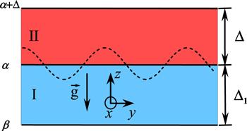
Figure 1. The RT model of two regions. The region I is from z = β to z = α, while the region II is from z = α to z = α + Δ. |
For simplicity and generality, we study the waves propagating only in the yoz plane, i.e. the wave number $\vec{k}=(0,{k}_{y},{k}_{z})$. Then the hydrodynamic equations to describe this kind of dusty plasma are as follows
$\begin{eqnarray}\displaystyle \frac{\partial {n}_{d}}{\partial t}+\displaystyle \frac{\partial \left({n}_{d}{v}_{d}\right)}{\partial y}+\displaystyle \frac{\partial \left({n}_{d}{w}_{d}\right)}{\partial z}=0,\end{eqnarray}$
$\begin{eqnarray}\begin{array}{l}\displaystyle \frac{\partial {v}_{d}}{\partial t}+{v}_{d}\displaystyle \frac{\partial {v}_{d}}{\partial y}+{w}_{d}\displaystyle \frac{\partial {v}_{d}}{\partial z}\\ \quad =\displaystyle \frac{{Z}_{d}e}{{m}_{d}}\left(\displaystyle \frac{\partial \phi }{\partial y}\ -\ {w}_{d}{B}_{x}\right)-\displaystyle \frac{1}{{m}_{d}{n}_{d}}\displaystyle \frac{\partial {P}_{d}}{\partial y},\end{array}\end{eqnarray}$
$\begin{eqnarray}\begin{array}{l}\displaystyle \frac{\partial {w}_{d}}{\partial t}+{v}_{d}\displaystyle \frac{\partial {w}_{d}}{\partial y}+{w}_{d}\displaystyle \frac{\partial {w}_{d}}{\partial z}\\ \quad =\displaystyle \frac{{Z}_{d}e}{{m}_{d}}\left(\displaystyle \frac{\partial \phi }{\partial z}+{v}_{d}{B}_{x}\right)-\displaystyle \frac{1}{{m}_{d}{n}_{d}}\displaystyle \frac{\partial {P}_{d}}{\partial z}-g,\end{array}\end{eqnarray}$
$\begin{eqnarray}\displaystyle \frac{{\partial }^{2}\phi }{\partial {y}^{2}}+\displaystyle \frac{{\partial }^{2}\phi }{\partial {z}^{2}}=\displaystyle \frac{e}{{\varepsilon }_{0}}\left({Z}_{d}{n}_{d}+{n}_{e}-{n}_{i}\right),\end{eqnarray}$
where nd refers to the number density of the dust particles, md is the mass of the dust particles, pd is the dust fluid pressure, vd, wd are the velocities of the dust fluid in the y direction and in the z direction, respectively, g is gravity acceleration constant, Zd is the number of charge of the electron residing on the dust particle and is assumed that it is a constant. $\vec{B}$ is the magnetic field intensity, and $\vec{B}={B}_{x}{\vec{e}}_{x}\ +\ {B}_{y}{\vec{e}}_{y}+{B}_{z}{\vec{e}}_{z}$.The incompressibility condition should be supplemented for the present system. It is valid because the observed dust flows are typically subsonic. The gravitational force on dust is not balanced by the dust pressure, but rather by the pressure of electrons and ions, which are coupled with the dust by electric fields
$\begin{eqnarray}{\rm{i}}{{kv}}_{d1}+\displaystyle \frac{{\rm{d}}{w}_{d1}}{{\rm{d}}z}=0.\end{eqnarray}$
We assume that
$\begin{eqnarray}{n}_{d}={n}_{d0}(z)+{n}_{d1}{{\rm{e}}}^{{\rm{i}}({ky}-\omega t)},\end{eqnarray}$
$\begin{eqnarray}B={B}_{0}+{B}_{1}{{\rm{e}}}^{{\rm{i}}({ky}-\omega t)},\end{eqnarray}$
$\begin{eqnarray}{v}_{d}={v}_{d1}{{\rm{e}}}^{{\rm{i}}({ky}-\omega t)},\end{eqnarray}$
$\begin{eqnarray}{w}_{d}={w}_{d1}{{\rm{e}}}^{{\rm{i}}({ky}-\omega t)},\end{eqnarray}$
$\begin{eqnarray}\phi ={\phi }_{1}{{\rm{e}}}^{{\rm{i}}({ky}-\omega t)},\end{eqnarray}$
where nd0 is the number density of the dust particle at equilibrium state, nd1 is the perturbed number density of the dust particle, vd1 and wd1 are the perturbed velocities of the dust fluid in the y and z directions, respectively, φ1 is the perturbed electric potential, B0 is a constant.In order to understand the RT instability of the system, we assume that the system is at an equilibrium state initially. Then by linearizing equations (2 )-(5 ), neglecting any nonlinear terms and substituting equations (7 )-(11 ) into equations (2 )-(5 ), we have
$\begin{eqnarray}-{\rm{i}}\omega {n}_{d1}+{w}_{d1}\displaystyle \frac{{\rm{d}}{n}_{d0}}{{\rm{d}}z}=0,\end{eqnarray}$
$\begin{eqnarray}-{\rm{i}}\omega {v}_{d1}=\displaystyle \frac{{Z}_{d}e}{{m}_{d}}\left({\rm{i}}k{\phi }_{1}-{w}_{d1}{B}_{0x}\right)-\displaystyle \frac{1}{{m}_{d}{n}_{d0}}{\rm{i}}{{kP}}_{d1},\end{eqnarray}$
$\begin{eqnarray}\begin{array}{l}-{\rm{i}}\omega {w}_{d1}=\displaystyle \frac{{Z}_{d}e}{{m}_{d}}\left(\displaystyle \frac{{\rm{d}}{\phi }_{1}}{{\rm{d}}z}+{v}_{d1}{B}_{0x}\right)\\ \quad -\displaystyle \frac{1}{{m}_{d}{n}_{d0}}\displaystyle \frac{{\rm{d}}{P}_{d1}}{{\rm{d}}z}-\displaystyle \frac{{n}_{d1}}{{n}_{d0}}g,\end{array}\end{eqnarray}$
$\begin{eqnarray}\begin{array}{l}-{k}^{2}{\phi }_{1}+\displaystyle \frac{{{\rm{d}}}^{2}{\phi }_{1}}{{\rm{d}}{z}^{2}}=\displaystyle \frac{e}{{\varepsilon }_{0}}\\ \quad \times \left[{Z}_{d}{n}_{d1}+\displaystyle \frac{e{\phi }_{1}}{{k}_{{\rm{B}}}}\left(\displaystyle \frac{{n}_{e0}}{{T}_{e}}+\displaystyle \frac{{n}_{i0}}{{T}_{i}}\right)\right].\end{array}\end{eqnarray}$
Simplifying equations (12 )-(15 ), we have
$\begin{eqnarray}\begin{array}{l}-{k}^{2}{\phi }_{1}+\displaystyle \frac{{{\rm{d}}}^{2}{\phi }_{1}}{{\rm{d}}{z}^{2}}=\displaystyle \frac{e}{{\varepsilon }_{0}}\\ \quad \times \left[\displaystyle \frac{{Z}_{d}{w}_{d1}}{{\rm{i}}\omega }\displaystyle \frac{{\rm{d}}{n}_{d0}}{{\rm{d}}z}+\displaystyle \frac{e{\phi }_{1}}{{k}_{{\rm{B}}}}\left(\displaystyle \frac{{n}_{e0}}{{T}_{e}}+\displaystyle \frac{{n}_{i0}}{{T}_{i}}\right)\right],\end{array}\end{eqnarray}$
$\begin{eqnarray}\begin{array}{l}\displaystyle \frac{{\rm{d}}}{{\rm{d}}z}\left({m}_{d}{n}_{d0}\displaystyle \frac{{\rm{d}}{w}_{d1}}{{\rm{d}}z}\right)-{k}^{2}\left({m}_{d}{n}_{d0}+{m}_{d}\displaystyle \frac{g}{{\omega }^{2}}\displaystyle \frac{{\rm{d}}{n}_{d0}}{{\rm{d}}z}\right){w}_{d1}\\ \quad =\ -\displaystyle \frac{{\rm{i}}{k}^{2}e}{\omega }\left[{Z}_{d}{n}_{d0}\displaystyle \frac{{\rm{d}}{\phi }_{1}}{{\rm{d}}z}-\displaystyle \frac{{\rm{d}}}{{\rm{d}}z}\left({Z}_{d}{n}_{d0}{\phi }_{1}\right)\right]\\ \quad -\displaystyle \frac{{ke}}{\omega }\left[{Z}_{d}{n}_{d0}{B}_{0x}\displaystyle \frac{{\rm{d}}{w}_{d1}}{{\rm{d}}z}-\displaystyle \frac{{\rm{d}}}{{\rm{d}}z}\left({Z}_{d}{n}_{d0}{w}_{d1}{B}_{0x}\right)\right].\end{array}\end{eqnarray}$
We now consider a dusty plasma in which there are two different regions, Region I: β < z < α and region II: α < z < α + Δ, see figure 1. We assume that the mass of dust particles in both regions is the same, while the number densities of the dusty plasma in both regions are different, nd0 = nd01 in region I. However, the number density of the dust particles varies with respect to space coordinate z as follows: ${n}_{d0}\left(z\right)={n}_{0}{{\rm{e}}}^{z/L}$ in region II, where constant L represents the number density gradient scale. Then we have from equations (16 ) and (17 )
$\begin{eqnarray}\displaystyle \frac{{{\rm{d}}}^{2}{\phi }_{1}}{{\rm{d}}{z}^{2}}-\left({k}^{2}+{\lambda }_{{}_{D}}^{-2}\right){\phi }_{1}=\displaystyle \frac{e}{{\rm{i}}\omega {\varepsilon }_{0}L}{Z}_{d}{n}_{0}{{\rm{e}}}^{z/L}{w}_{d1},\end{eqnarray}$
$\begin{eqnarray}\begin{array}{l}\displaystyle \frac{{{\rm{d}}}^{2}{w}_{d1}}{{\rm{d}}{z}^{2}}+\displaystyle \frac{1}{L}\displaystyle \frac{{\rm{d}}{w}_{d1}}{{\rm{d}}z}-{k}^{2}\left(1+\displaystyle \frac{g}{L{\omega }^{2}}\right){w}_{d1}\\ \quad =\displaystyle \frac{{\rm{i}}{k}^{2}{{eZ}}_{d}}{\omega {m}_{d}L}{\phi }_{1}-\displaystyle \frac{{{keZ}}_{d}}{\omega {m}_{d}L}{w}_{d1}{B}_{0x},\end{array}\end{eqnarray}$
where ${\lambda }_{D}={\left(\tfrac{{n}_{e0}{e}^{2}}{{\varepsilon }_{0}{k}_{{\rm{B}}}{T}_{e}}+\tfrac{{n}_{i0}{e}^{2}}{{\varepsilon }_{0}{k}_{{\rm{B}}}{T}_{i}}\right)}^{-1/2}$.Rewriting equations (18 ) and (19 ), we have
$\begin{eqnarray}\begin{array}{l}\displaystyle \frac{{{\rm{d}}}^{4}{w}_{d1}}{{\rm{d}}{z}^{4}}+\displaystyle \frac{1}{L}\displaystyle \frac{{{\rm{d}}}^{3}{w}_{d1}}{{\rm{d}}{z}^{3}}\\ \quad -\left[{k}^{2}\left(1+\displaystyle \frac{g}{L{\omega }^{2}}\right)-\displaystyle \frac{{{keZ}}_{d}}{\omega {m}_{d}L}{B}_{0x}+\left({k}^{2}+{\lambda }_{{}_{D}}^{-2}\right)\right]\displaystyle \frac{{{\rm{d}}}^{2}{w}_{d1}}{{\rm{d}}{z}^{2}}\\ \quad -\left({k}^{2}+{\lambda }_{{}_{D}}^{-2}\right)\displaystyle \frac{1}{L}\displaystyle \frac{{\rm{d}}{w}_{d1}}{{\rm{d}}z}\\ \quad +\left({k}^{2}+{\lambda }_{{}_{D}}^{-2}\right)\left[{k}^{2}\left(1+\displaystyle \frac{g}{L{\omega }^{2}}\right)-\displaystyle \frac{{{keZ}}_{d}}{\omega {m}_{d}L}{B}_{0x}\right]{w}_{d1}\\ \quad =\,\displaystyle \frac{{k}^{2}{e}^{2}{Z}_{{}_{d}}^{2}}{{\varepsilon }_{0}{\omega }^{2}{L}^{2}{m}_{d}}{n}_{0}{{\rm{e}}}^{z/L}{w}_{d1}.\end{array}\end{eqnarray}$
In order to know how the growth rate depends on the plasma parameters, we choose some typical plasma parameters as reported experimentally in the previous work [18]. We use e = 1.6 × 10⁻¹⁹ C, ϵ0 = 8.854 × 10⁻¹² F m−1, Zd = 4500, md ∼ 10−14 kg, n0 ∼ 1011 m−3, L = 2.0 m, we find that the order of the right hand side of equation (20 ) is $\tfrac{{k}^{2}{e}^{2}{Z}_{{}_{d}}^{2}{n}_{0}}{{\varepsilon }_{0}{L}^{2}{\omega }^{2}{m}_{d}}\sim {10}^{-3}$ when k ≈ 0.1, while the order of the last term of the left hand side of equation (20 ) is $\left({k}^{2}+{\lambda }_{{}_{D}}^{-2}\right)\left({k}^{2}\left(1+\tfrac{g}{L{\omega }^{2}}\right)+\tfrac{{{keZ}}_{d}}{\omega {m}_{d}L}{B}_{0x}\right)\sim {10}^{6}$. Due to this reason, we neglect the right hand side of equation (20 ). Then, the eigenvalues corresponding to equation (20 ) are as follows
$\begin{eqnarray}\displaystyle \frac{3}{{L}^{2}}+8\left[{k}^{2}\left(1+\displaystyle \frac{g}{L{\omega }^{2}}\right)-\displaystyle \frac{{{keZ}}_{d}}{\omega {m}_{d}L}{B}_{0x}+\left({k}^{2}+{\lambda }_{{}_{D}}^{-2}\right)\right]=0.\end{eqnarray}$
The dispersion relation is
$\begin{eqnarray}{\omega }^{2}=\displaystyle \frac{{\left(\tfrac{8{{keZ}}_{d}{{LB}}_{0x}}{{m}_{d}}\right)}^{2}-32{k}^{2}{gL}\left[3+8{k}^{2}{L}^{2}+8{L}^{2}\left({k}^{2}+{\lambda }_{{}_{D}}^{-2}\right)\right]}{4{\left[3+8{k}^{2}{L}^{2}+8{L}^{2}\left({k}^{2}+{\lambda }_{{}_{D}}^{-2}\right)\right]}^{2}}.\end{eqnarray}$
The growth rate of the RT instability can be expressed as follows
$\begin{eqnarray}\gamma =\sqrt{-\displaystyle \frac{{\left(\tfrac{8{{keZ}}_{d}{{LB}}_{0x}}{{m}_{d}}\right)}^{2}-32{k}^{2}{gL}\left[3+8{k}^{2}{L}^{2}+8{L}^{2}\left({k}^{2}+{\lambda }_{{}_{D}}^{-2}\right)\right]}{4{\left[3+8{k}^{2}{L}^{2}+8{L}^{2}\left({k}^{2}+{\lambda }_{{}_{D}}^{-2}\right)\right]}^{2}}}.\end{eqnarray}$
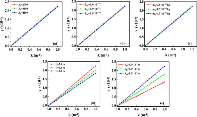
Figure 2 shows the dependence of the growth rate of the RT instability on the wave number k for different Zd in figure 2 (a), different B0x in figure 2 (b), different md in figure 2 (c), different values of L in figure 2 (d), different λD in figure 2 (e). The plasma parameters are chosen from the previous work [18] md = 1.3 × 10⁻¹⁴ kg, B0x = 0.4 × 10⁻⁴ T, L = 2.0 m, λD = 1.0 × 10⁻⁴ m in figure 2 (a). md = 1.3 × 10⁻¹⁴ kg, Zd = 4500, λD = 1.0 × 10⁻⁴ m in figure 2 (b). Zd = 4500, B0x = 0.4 × 10⁻⁴ T, L=2.0 m, λD = 1.0 × 10⁻⁴ m in figure 2 (c). md = 1.3 × 10⁻¹⁴ kg, Zd = 4500, B0x = 0.4 × 10⁻⁴ T, λD = 1.0 × 10⁻⁴ m in figure 2 (d). md = 1.3 × 10⁻¹⁴ kg, Zd = 4500, B0x = 0.4 × 10⁻⁴ T, L = 2.0 m in figure 2 (e).
Figure 2. (a) Dependence of the growth rate of the RT instability on the wave number k for different parameters of Zd = 2700, 3600, 4500, respectively. (b) Dependence of the growth rate of the RT instability on the wave number k for different parameters of B0x = 0.4 × 10⁻⁴ T, 0.5 × 10⁻⁴ T, 0.6 × 10⁻⁴ T, respectively. (c) Dependence of the growth rate of the RT instability on the wave number k for different parameters of md = 3.6 × 10⁻¹⁵ kg, 8.5 × 10⁻¹⁵ kg, 1.3 × 10⁻¹⁴ kg, respectively. (d) Dependence of the growth rate of the RT instability on the wave number k for different parameters of L = 2.0 m, 2.5 m, 3.0 m, respectively. (e) Dependence of the growth rate of the RT instability on the wave number k for different parameters of λD = 6 × 10⁻⁵ m, 8 × 10⁻⁵ m, 1 × 10⁻⁴ m, respectively. |
Notice from figure 2 that the growth rate of the RT instability increases as the wave number k increases. It suggests that the shorter the wavelength, the larger the growth rate. It is noted from figures 2(a)-(c) that the magnitude of the electric charge on a dust particle Zd, the external magnetic field B0x and the mass of a dust particle md almost have no effect on the RT instability. Similarly, in order to know how the growth rate depends on the plasma parameters, we choose some typical plasma parameters as reported experimentally in the previous work [18]. We use e = 1.6 × 10⁻¹⁹ C, Zd = 4500, L = 2.0m, k ≈ 0.1, md ∼ 10−14 kg, B0x ∼ 10−4 T, λD ∼ 10−4 m, and find that the order of the first term of the numerator of equation (23 ) is $\tfrac{8{{keZ}}_{d}{{LB}}_{0x}}{{m}_{d}}\sim {10}^{-6}$, while the order of the second term of the numerator of equation (23 ) is $32{k}^{2}{gL}[3+8{k}^{2}{L}^{2}+8{L}^{2}({k}^{2}+{\lambda }_{D}^{-2})]\sim {10}^{10}$. Due to this reason, we neglect the first term of the numerator of equation (23 ). Therefore, the magnitude of the electric charge on a dust particle Zd, the external magnetic field B0x and the mass of a dust particle md almost have no effect on the RT instability. However, it indicates from figures 2(d) and (e) that both the parameters L and λD obviously affect the growth rate of the RT instability. It is found that the growth rate decreases as L increases. It suggests that the larger the number density gradient scale, the less the growth rate of the RT instability. Moreover, the growth rate increases as λD increases. It seems that the larger the Debye length, the larger the growth rate of the RT instability.
It seems that the number density and the temperature of both electrons and ions can affect the RT instability. It indicates that the larger the number densities of both electrons and ions, the smaller the growth rate, while the higher the temperatures of both electrons and ions, the larger the growth rate. It is found that the RT instability and its growth rate not only depend on the region parameters (the external magnetic field, the region length and its gradient) and the dust particles parameters (the number density, the mass and the charge of the dust particle), but also on both electron and ion characters (the number densities, the temperatures of both electrons and ions).
2.2. RT instability in an ion-electron plasma
For comparison, we now consider an ion-electron plasma consisting of electrons and ions, which has been studied extensively in previous works [62–66]. In order to investigate the RT instability in an ion-electron plasma, we assume that the electrons follow the Boltzmann distribution, ${n}_{e}={n}_{e0}\exp \left(\tfrac{e\phi }{{k}_{{\rm{B}}}{T}_{e}}\right)$, while the ions are treated as a fluid. The same model is considered for ion-electron plasma, as shown in figure 1. For simplicity and generality, we also study waves propagating only in the yoz plane, i.e. the wave number $\vec{k}=(0,{k}_{y},{k}_{z})$. Then the hydrodynamic equations to describe this kind of ion-electron plasma are as follows
$\begin{eqnarray}\displaystyle \frac{\partial {n}_{i}}{\partial t}+\displaystyle \frac{\partial \left({n}_{i}{v}_{i}\right)}{\partial y}+\displaystyle \frac{\partial \left({n}_{i}{w}_{i}\right)}{\partial z}=0,\end{eqnarray}$
$\begin{eqnarray}\begin{array}{l}\displaystyle \frac{\partial {v}_{i}}{\partial t}+{v}_{i}\displaystyle \frac{\partial {v}_{i}}{\partial y}+{w}_{i}\displaystyle \frac{\partial {v}_{i}}{\partial z}\\ \quad =\displaystyle \frac{e}{{m}_{i}}\left(-\displaystyle \frac{\partial \phi }{\partial y}\ +\ {w}_{i}{B}_{x}\right)-\displaystyle \frac{1}{{m}_{i}{n}_{i}}\displaystyle \frac{\partial {P}_{i}}{\partial y},\end{array}\end{eqnarray}$
$\begin{eqnarray}\begin{array}{l}\displaystyle \frac{\partial {w}_{i}}{\partial t}+{v}_{i}\displaystyle \frac{\partial {w}_{i}}{\partial y}+{w}_{i}\displaystyle \frac{\partial {w}_{i}}{\partial z}\\ \quad =\displaystyle \frac{e}{{m}_{i}}\left(-\displaystyle \frac{\partial \phi }{\partial z}-{v}_{i}{B}_{x}\right)-\displaystyle \frac{1}{{m}_{i}{n}_{i}}\displaystyle \frac{\partial {P}_{i}}{\partial z}-g,\end{array}\end{eqnarray}$
$\begin{eqnarray}\displaystyle \frac{{\partial }^{2}\phi }{\partial {y}^{2}}+\displaystyle \frac{{\partial }^{2}\phi }{\partial {z}^{2}}=\displaystyle \frac{e}{{\varepsilon }_{0}}\left({n}_{e}-{n}_{i}\right),\end{eqnarray}$
where ni refers to the number density of ions, mi is the mass of ions, pi is the ion fluid pressure, vi, wi are the velocities of ion fluid in the y direction and in the z direction, respectively, g is gravity acceleration constant, φ is electric potential, $\vec{B}$ is the magnetic field intensity, $\vec{B}={B}_{x}{\vec{e}}_{x}\ +\ {B}_{y}{\vec{e}}_{y}+{\vec{B}}_{z}{\vec{e}}_{z}$.Using the incompressibility condition,
$\begin{eqnarray}{\rm{i}}{{kv}}_{i1}+\displaystyle \frac{{\rm{d}}{w}_{i1}}{{dz}}=0.\end{eqnarray}$
We assume that
$\begin{eqnarray}{n}_{i}={n}_{i0}(z)+{n}_{i1}{{\rm{e}}}^{{\rm{i}}({ky}-\omega t)},\end{eqnarray}$
$\begin{eqnarray}B={B}_{0}+{B}_{1}{{\rm{e}}}^{{\rm{i}}({ky}-\omega t)},\end{eqnarray}$
$\begin{eqnarray}{v}_{i}={v}_{i1}{{\rm{e}}}^{{\rm{i}}({ky}-\omega t)},\end{eqnarray}$
$\begin{eqnarray}{w}_{i}={w}_{i1}{{\rm{e}}}^{{\rm{i}}({ky}-\omega t)},\end{eqnarray}$
$\begin{eqnarray}\phi ={\phi }_{1}{{\rm{e}}}^{{\rm{i}}({ky}-\omega t)},\end{eqnarray}$
where ni0 is the number density of ions at equilibrium state, ni1 is the perturbed number density of ions, vi1 and wi1 are the perturbed velocities of the ion in the y and z directions respectively, φ1 is the perturbed potential, B0 is a constant.In order to understand the RT instability of the system, we assume that the system is at an equilibrium state initially. Then by linearizing equations (24 )-(27 ), neglecting any nonlinear terms and substituting equations (28 )-(33 ) into equations (24 )-(27 ), we have
$\begin{eqnarray}-{\rm{i}}\omega {n}_{i1}+{w}_{i1}\displaystyle \frac{{\rm{d}}{n}_{i0}}{{\rm{d}}z}=0,\end{eqnarray}$
$\begin{eqnarray}-{\rm{i}}\omega {v}_{i1}=\displaystyle \frac{e}{{m}_{i}}\left(-{\rm{i}}k{\phi }_{1}+{w}_{i1}{B}_{0x}\right)-\displaystyle \frac{1}{{m}_{i}{n}_{i0}}{\rm{i}}{{kP}}_{i1},\end{eqnarray}$
$\begin{eqnarray}-{\rm{i}}\omega {w}_{i1}=\displaystyle \frac{e}{{m}_{i}}\left(-\displaystyle \frac{{\rm{d}}{\phi }_{1}}{{\rm{d}}z}-{v}_{i1}{B}_{0x}\right)-\displaystyle \frac{1}{{m}_{i}{n}_{i0}}\displaystyle \frac{{\rm{d}}{P}_{i1}}{{\rm{d}}z}-\displaystyle \frac{{n}_{i1}}{{n}_{i0}}g,\end{eqnarray}$
$\begin{eqnarray}-{k}^{2}{\phi }_{1}+\displaystyle \frac{{{\rm{d}}}^{2}{\phi }_{1}}{{\rm{d}}{z}^{2}}=\displaystyle \frac{e}{{\varepsilon }_{0}}\left(\displaystyle \frac{{n}_{e0}e{\phi }_{1}}{{k}_{{\rm{B}}}{T}_{e}}-{n}_{i1}\right).\end{eqnarray}$
Simplifying equations (34 )-(37 ), we have
$\begin{eqnarray}\begin{array}{l}\displaystyle \frac{{\rm{d}}}{{\rm{d}}z}({m}_{i}{n}_{i0}\displaystyle \frac{{\rm{d}}{w}_{i1}}{{\rm{d}}z})-{k}^{2}({m}_{i}{n}_{i0}+{m}_{i}\displaystyle \frac{g}{{\omega }^{2}}\displaystyle \frac{{\rm{d}}{n}_{i0}}{{\rm{d}}z}){w}_{i1}\\ \quad =\displaystyle \frac{{\rm{i}}{k}^{2}e}{\omega }\left[{n}_{i0}\displaystyle \frac{{\rm{d}}{\phi }_{1}}{{\rm{d}}z}-\displaystyle \frac{{\rm{d}}}{{\rm{d}}z}({n}_{i0}{\phi }_{1})\right]-\displaystyle \frac{{ke}}{\omega }\\ \quad \times \left[{n}_{i0}{B}_{0x}\displaystyle \frac{{\rm{d}}{w}_{i1}}{{\rm{d}}z}-\displaystyle \frac{{\rm{d}}}{{\rm{d}}z}\left({n}_{i0}{w}_{i1}{B}_{0x}\right)\right],\end{array}\end{eqnarray}$
$\begin{eqnarray}-{k}^{2}{\phi }_{1}+\displaystyle \frac{{{\rm{d}}}^{2}{\phi }_{1}}{{\rm{d}}{z}^{2}}=\displaystyle \frac{e}{{\varepsilon }_{0}}\left(\displaystyle \frac{{n}_{e0}e{\phi }_{1}}{{k}_{{\rm{B}}}{T}_{e}}-\displaystyle \frac{{w}_{i1}}{{\rm{i}}\omega }\displaystyle \frac{{\rm{d}}{n}_{i0}}{{\rm{d}}z}\right).\end{eqnarray}$
Similarly, we consider an ion-electron plasma in which there are two different regions. Region I: β < z < α and region II: α < z < α + Δ, see in figure 1, where ni0 = ni01 in region I. While ${n}_{i0}\left(z\right)={n}_{0}{{\rm{e}}}^{z/L}$ in region II. Then we have from equations (38 ) and (39 )
$\begin{eqnarray}\begin{array}{l}\displaystyle \frac{{{\rm{d}}}^{2}{w}_{i1}}{{\rm{d}}{z}^{2}}+\displaystyle \frac{1}{L}\displaystyle \frac{{\rm{d}}{w}_{i1}}{{\rm{d}}z}-{k}^{2}\left(1+\displaystyle \frac{g}{L{\omega }^{2}}\right){w}_{i1}\\ \quad =-\displaystyle \frac{{\rm{i}}{k}^{2}e}{\omega {m}_{i}L}{\phi }_{1}+\displaystyle \frac{{ke}}{\omega {m}_{i}L}{w}_{i1}{B}_{0x},\end{array}\end{eqnarray}$
$\begin{eqnarray}-{k}^{2}{\phi }_{1}+\displaystyle \frac{{{\rm{d}}}^{2}{\phi }_{1}}{{\rm{d}}{z}^{2}}=\displaystyle \frac{{e}^{2}{\phi }_{1}}{{\varepsilon }_{0}{k}_{{\rm{B}}}{T}_{e}}{n}_{0}{{\rm{e}}}^{z/L}-\displaystyle \frac{e}{{\rm{i}}\omega {\varepsilon }_{0}L}{n}_{0}{{\rm{e}}}^{z/L}{w}_{i1}.\end{eqnarray}$
Rewriting equations (40 ) and (41 ), we have
$\begin{eqnarray}\begin{array}{l}\displaystyle \frac{{{\rm{d}}}^{4}{w}_{i1}}{{\rm{d}}{z}^{4}}+\displaystyle \frac{1}{L}\displaystyle \frac{{{\rm{d}}}^{3}{w}_{i1}}{{\rm{d}}{z}^{3}}-\left[{k}^{2}\left(1+\displaystyle \frac{g}{L{\omega }^{2}}\right)\right.\\ \quad \left.+\displaystyle \frac{{{keB}}_{0x}}{\omega {m}_{i}L}+\left({k}^{2}+\displaystyle \frac{{e}^{2}{n}_{0}{{\rm{e}}}^{z/L}}{{\varepsilon }_{0}{k}_{{\rm{B}}}{T}_{e}}\right)\right]\displaystyle \frac{{{\rm{d}}}^{2}{w}_{i1}}{{\rm{d}}{z}^{2}}\\ \quad -\left({k}^{2}+\displaystyle \frac{{e}^{2}{n}_{0}{{\rm{e}}}^{z/L}}{{\varepsilon }_{0}{k}_{{\rm{B}}}{T}_{e}}\right)\displaystyle \frac{1}{L}\displaystyle \frac{{\rm{d}}{w}_{i1}}{{\rm{d}}z}+\left({k}^{2}+\displaystyle \frac{{e}^{2}{n}_{0}{{\rm{e}}}^{z/L}}{{\varepsilon }_{0}{k}_{{\rm{B}}}{T}_{e}}\right)\\ \quad \times \left[{k}^{2}\left(1+\displaystyle \frac{g}{L{\omega }^{2}}\right)+\displaystyle \frac{{{keB}}_{0x}}{\omega {m}_{i}L}\right]{w}_{i1}=\displaystyle \frac{{k}^{2}{e}^{2}{n}_{0}{{\rm{e}}}^{z/L}}{{\varepsilon }_{0}{\omega }^{2}{L}^{2}{m}_{i}}{w}_{i1}.\end{array}\end{eqnarray}$
In order to know how the growth rate depends on the plasma parameters, we choose some typical plasma parameters as reported experimentally in the previous work [24]. If we choose e = 1.6 × 10⁻¹⁹ C, ϵ0 = 8.854 × 10⁻¹² F m−1, mi ∼ 10−27 kg, n0 ∼ 1014 m−3, L = 2.0 m, we find that the order of the left hand side of equation (42 ) $\tfrac{1}{L}\sim {10}^{-1},{k}^{2}\sim {10}^{-2},{k}^{2}\left(1+\tfrac{g}{L{\omega }^{2}}\right)\sim {10}^{-2},\tfrac{{{keB}}_{0x}}{\omega {m}_{i}L}\sim {10}^{-5}$, $\tfrac{{e}^{2}{n}_{0}}{{\varepsilon }_{0}{k}_{{\rm{B}}}{T}_{e}}\sim {10}^{6}$ when k ≈ 0.1, while the order of the right hand side of equation (42 ) is $\tfrac{{k}^{2}{e}^{2}{n}_{0}}{{\varepsilon }_{0}{\omega }^{2}{L}^{2}{m}_{i}}\sim {10}^{-3}$. Due to this reason, we neglect the small coefficients of equation (42 ). we have
$\begin{eqnarray}\displaystyle \frac{{{\rm{d}}}^{2}{w}_{i1}}{{\rm{d}}{z}^{2}}+\displaystyle \frac{1}{L}\displaystyle \frac{{\rm{d}}{w}_{i1}}{{\rm{d}}z}-\left[{k}^{2}\left(1+\displaystyle \frac{g}{L{\omega }^{2}}\right)+\displaystyle \frac{{{keB}}_{0x}}{\omega {m}_{i}L}\right]{w}_{i1}=0.\end{eqnarray}$
Moreover, the eigenvalues corresponding to equation (43 ) are as follows
$\begin{eqnarray}\displaystyle \frac{1}{{L}^{2}}+4\left[{k}^{2}\left(1+\displaystyle \frac{g}{L{\omega }^{2}}\right)+\displaystyle \frac{{{keB}}_{0x}}{\omega {m}_{i}L}\right]=0.\end{eqnarray}$
The dispersion relation is
$\begin{eqnarray}{\omega }^{2}=\displaystyle \frac{{\left(\tfrac{4{{keLB}}_{0x}}{{m}_{i}}\right)}^{2}-16{k}^{2}{gL}\left(1+4{k}^{2}{L}^{2}\right)}{4{\left(1+4{k}^{2}{L}^{2}\right)}^{2}}.\end{eqnarray}$
It seems from equation (45 ) that ω2 > 0 when the equation of ${B}_{0x}^{2}\geqslant g(1+4{k}^{2}{L}^{2})\displaystyle \frac{{m}_{i}^{2}}{{e}^{2}L}$ is satisfied. It is estimated that when the external magnetic field B0x is larger than 10−8 T, ω2 > 0 may be satisfied since $\displaystyle \frac{{m}_{i}}{e}\sim {10}^{-8}$. Then, we conclude that the external magnetic field can strongly refrain the RT instability for electron-ion plasma. This result is different from that for a dusty plasma about which the external magnetic field only has a weak effect to refrain the RT instability.
When B0x = 0, the dispersion relation is
$\begin{eqnarray}{\omega }^{2}=-\displaystyle \frac{4{k}^{2}{gL}}{1+4{k}^{2}{L}^{2}}.\end{eqnarray}$
The growth rate of the RT instability can be expressed as follows
$\begin{eqnarray}\gamma =\sqrt{\displaystyle \frac{4{k}^{2}{gL}}{1+4{k}^{2}{L}^{2}}}.\end{eqnarray}$
It seems that the dispersion relation equation (46 ) is consistent with that of the general fluid [67] and therefore there is RT instability.
2.3. Effects of the charge to mass ratio of charged fluids on the growth rate of the RT instability
The present results show that an external magnetic field is more effective on suppressing the RT instability in ion-electron plasma than that in dusty plasma. The explanation for this difference can be inferred by examining both equations (23 ) and (45 ). We can define a refrain factor to RT instability which is given by $\sigma \sim \displaystyle \frac{Q}{M}{B}_{0x}$, where Q is the electric charge of the charged particle and M is the mass of the charged particle. Put simply, the degree to which the RT instability is suppressed depends on the product of the external magnetic field and the charge-mass ratio of the charged particles. Due to the much larger charge-mass ratio of ions compared to dust particles, the effect of the external magnetic field in suppressing the RT instability is much more pronounced in ion-electron plasma than that in dusty plasma. In other words, the greater the charge-mass ratio of the charged particle, the stronger the effect of the magnetic field in suppressing the RT instability.
3. Summary and conclusion
The present paper provides a theoretical investigation of the RT instability in different kinds of charged fluid. One is a dusty plasma, while the other is ion-electron plasma. It is found that the charge-mass ratio of charged particles in a charged fluid plays a crucial role in the RT instability and its growth rate. It appears that a larger charge-mass ratio leads to a stronger effect of the external magnetic field in restraining the RT instability. Consequently, the effect of the magnetic field in refraining the RT instability is much more significant in ion-electron plasma compared to dusty plasma due to the ions' larger charge-mass ratio.
It is also found that, for a dusty plasma, the growth rate of the RT instability increases as the perturbed wave number increases. Moreover, the RT instability and its growth rate depend not only on the external parameters of the region (the external magnetic field, the length of the region, and its gradient), the parameters of the dust particles (the number density, the mass, and the charge), but also on the characteristics of both the electrons and ions such as their number densities and their temperatures.
Currently, our research may have potential applications. For example, it is almost impossible to refrain RT instability by an external magnetic field for a dusty plasma. However, it is easy to refrain the RT instability by an external magnetic field for an ion-electron plasma.