Welcome to visit Communications in Theoretical Physics,
Others

Lyapunov functions for studying global asymptotic stability of two rumor spreading models

  • Manh Tuan Hoang
Expand
  • Department of Mathematics, FPT University, Hoa Lac Hi-Tech Park, Km29 Thang Long Blvd, Hanoi, Vietnam

Received date: 2023-05-23

  Revised date: 2023-08-29

  Accepted date: 2023-08-29

  Online published: 2023-09-20

Copyright

© 2023 Institute of Theoretical Physics CAS, Chinese Physical Society and IOP Publishing

Abstract

In a previous work (2018, Commun. Theor. Phys. 70, 795-802), a new compartment model for the spreading of rumors was introduced and analyzed. However, only the local asymptotic stability of this model was discussed. In the present work, we first provide a rigorous mathematical analysis for the global asymptotic stability (GAS) of the above-mentioned rumor spreading model. By constructing suitable Lyapunov candidate functions, we obtain the GAS of a rumor-free (boundary) equilibrium point and a unique rumor-spreading (positive) equilibrium point. After that, we utilize the approach based on the Lyapunov candidate functions to study the GAS of another rumor spreading model with control strategies, which was proposed in (2022, Physica A 606, 128157). As an important consequence, the GAS of the rumor spreading model with control strategies is determined fully without resorting to technical hypotheses used in the benchmark work. Lastly, the theoretical findings are supported by a set of illustrative numerical examples. The obtained results not only improve the ones constructed in the two above-mentioned benchmark papers but also can be extended to study the global dynamics of other rumor propagation models in the context of both integer-order and fractional-order derivatives.

Cite this article

Manh Tuan Hoang . Lyapunov functions for studying global asymptotic stability of two rumor spreading models[J]. Communications in Theoretical Physics, 2023 , 75(10) : 105802 . DOI: 10.1088/1572-9494/acf48d

1. Introduction

It is well-known that controlling rumors is an important social issue, especially in the context of the rapidly evolving Internet and social media sites and platforms For this reason, many mathematicians and engineers have studied a broad range of mathematical models based on basic principles of compartment epidemiological models for describing the transmission of rumors (see, for example, [112]). These models have various useful applications in real-world situations and can suggest effective and suitable strategies to control the spreading of rumors. It is important to note that rumors are often spread in community and social networks; hence, there is a high similarity between the spreading of rumors and the transmission of infectious diseases (see, for instance, [1315]).
In a previous work [1], Dong and Huang proposed a new rumor spreading model, which is based on characteristics of the transmission of rumors in online social networks and can be considered as a modification of the well-known SIS epidemic models. In this model, the total population N is divided into two compartments according to their statuses with respect to rumors, namely the susceptible (health) class S that contains network users who are not under the influence of some rumor message at some time and the infected (transmission) class I containing network users who are in the influence of some rumor message at some time so that they involve in the message propagation. Then, the following model was formulated by using basic ideas of mathematical epidemiology and suitable technical hypotheses
$\begin{eqnarray}\begin{array}{rcl}\displaystyle \frac{{\rm{d}}S}{{\rm{d}}t} & = & {bS}+(b+\sigma )I-{{bS}}^{2}-(\beta +b){SI},\\ \displaystyle \frac{{\rm{d}}I}{{\rm{d}}t} & = & -\sigma I-{{bI}}^{2}+(\beta -b){SI},\end{array}\end{eqnarray}$
Here, all the parameters are assumed to be positive due to biological and epidemiological reasons. It is important to remark that the changing total user number N(t) in the online social networks was assumed to satisfy the logistic differential equation dN/dt = bN(1 − N) since the network population grows but definitely has the global human population as its upper ceiling, where b is the net growth rate of users and is determined by the difference of the registration rate of new users and deactivation rate of users. We refer the readers to [1] for more details of the model (5) and its derivation.
It was proved in [1] that the model (1) always has a rumor-free equilibrium point F0 = (1, 0) for all the values of the parameters and a unique (positive) rumor-spreading equilibrium point, which is given by ${F}_{* }=({S}_{* },{I}_{* })\,=\left((b+\sigma )/\beta ,1-(b+\sigma )/\beta \right)$, exists if β > b + σ. It should be emphasized that in [1] only local asymptotic stability of F* was established but numerical examples suggested that this equilibrium point may be not only locally asymptotically stable but also globally asymptotically stable (see section 4 in [1]). It is worth noting that the analysis of global asymptotic stability (GAS) of dynamical systems governed by differential equations is an important and prominent problem with many applications in both theory and practice [1619].
Motivated by the above reason, in the first part of this work, we provide a rigorous mathematical analysis for the GAS of the compartment model (1). By using suitable Lyapunov functions, we obtain the GAS of the rumor-free and rumor-spreading equilibrium points of the model (1). The obtained results improve the stability analysis performed in [1].
After establishing the complete GAS of the model (1), we consider another rumor spreading model with discontinuous control strategies introduced in [12]. This model is a combination of the model (1) with control strategies and is given by
$\begin{eqnarray}\begin{array}{rcl}\displaystyle \frac{{\rm{d}}S}{{\rm{d}}t} & = & {aS}-{{aS}}^{2}+(a+b)I-(\sigma +a){SI}+q\varphi (I)I,\\ \displaystyle \frac{{\rm{d}}I}{{\rm{d}}t} & = & -{bI}-{{aI}}^{2}+(\sigma -a){SI}-q\varphi (I)I,\end{array}\end{eqnarray}$
where φ(I) is called a control function and satisfies the following properties
i

(i)$\varphi :{{\mathbb{R}}}_{+}\to {{\mathbb{R}}}_{+}$ and has a limited number of jump discontinuities in every compact interval;

ii

(ii)φ and is non-decreasing and φ(x) ∈ [0, 1] for all x ∈ [0, 1].

The derivation and practical meanings of the control function φ(I) were explained in [12].
In [12], stability analysis of equilibrium points and global convergence in finite time of the model (2) were studied. In particular, it was shown that a rumor-free equilibrium E0 = (1, 0) always exists and it is globally asymptotically stable if σ < a + b + qφ(0) (see theorem 4.1 in [12]); and if σabq > 0, then at least one rumor-spreading (positive) equilibrium point E* = (S*, I*) exists (see theorem 3.1 in [12]) and it is globally asymptotically stable whenever (see theorem 4.2 in [12])
$\begin{eqnarray}2q+a-\sigma -{{qI}}^{* }\gt 0\end{eqnarray}$
and
$\begin{eqnarray}\begin{array}{l}a\left[{{aS}}^{* }-\displaystyle \frac{\sigma +a}{2}+(\sigma +a){I}^{* }-\displaystyle \frac{{{qI}}^{* }}{2}\right]\\ \quad \gt (a+q+b)(\sigma -a).\end{array}\end{eqnarray}$
Although the conditions (3) and (4) may be not difficult to be verified, they make the parameter space limited; moreover, stability analysis of many epidemic models suggested that positive equilibrium points are often globally asymptotically stable provided they exist (see, for instance, [2022]). Therefore, it is reasonable to predict that conditions (3) and (4) may be technical hypotheses and can be released.
By the above reason, in the second part of this work, we utilize the approach based on the Lyapunov functions, which was used to analyze the GAS of the model (1), to investigate the GAS of the equilibrium points of the model (2). As expected, we obtain the complete GAS of the model (2) without resorting to the technical hypotheses (3) and (4). Hence, the stability analysis in [12] is improved.
As we mentioned above, the GAS analysis of dynamical systems is an essential problem with many useful applications in real-world situations but it is not a trivial task in general. It is well-known that the Lyapunov stability theory has been considered as one of the most successful approaches to this problem [1619]. However, an indispensable requirement of this approach is the construction of suitable Lyapunov function candidates but there is no general technique for constructing such Lyapunov functions. In the present work, by transforming the model (1) to the new system (5) and utilizing well-known Lyapunov functions suggested in previous works, namely linear Lyapunov functions and Voltera-Lyapunov functions (see, e.g. [2327]), we construct appropriate Lyapunov functions to establish the GAS of the rumor spreading models (1) and also (2). Moreover, the constructed Lyapunov functions can be utilized to study the stability properties of extensions of the rumor spreading models in the context of fractional-order models. This is an important advantage of the used Lyapunov functions.
Lastly, in the third part of this work, we report a set of illustrative numerical examples to support the theoretical findings. The obtained results indicate that the numerical examples are consistent with the theoretical assertions.
The plan of this work is as follows:
In section 2, we analyze the complete GAS of the model (1). The GAS analysis of the model (2) is performed in section 3. Section 4 reports a set of illustrative numerical examples. Some conclusions and discussions are presented in the last section.

2. Stability analysis of the model (1)

In this section, we analyze the GAS of the model (1). First, let us denote by N the total population, that is, N(t) = S(t) + I(t) for t ≥ 0. Then, the model (1) can be represented in the from
$\begin{eqnarray}\begin{array}{rcl}\displaystyle \frac{{\rm{d}}N}{{\rm{d}}t} & = & {bN}(1-N),\\ \displaystyle \frac{{\rm{d}}I}{{\rm{d}}t} & = & -\sigma I-\beta {I}^{2}+(\beta -b){NI}.\end{array}\end{eqnarray}$
Here, a feasible region of the model (5) is given by
$\begin{eqnarray}{\rm{\Omega }}=\{(N,I)| 0\leqslant N\leqslant 1,\quad 0\leqslant I\leqslant 1\}.\end{eqnarray}$
It is easy to verify that the model (5) always has two rumor-free equilibrium points E0 = (N0, I0) = (1, 0) and E1 = (N1, I1) = (0, 0) while a unique (positive) rumor-spreading equilibrium point ${E}_{* }=({N}_{* },{I}_{* })=\left(1,\,1-\displaystyle \frac{b+\sigma }{\beta }\right)$ exists if and only if b + σ < β. Before establishing the GAS, we examine the local asymptotic stability of the model (5) based on Lyapunov's indirect method (see [16], theorem 4.7).

i

(i)The equilibrium point ${E}_{1}=(0,0)$ is always unstable.

ii

(ii)The rumor-free equilibrium point ${E}_{0}=(1,0)$ is locally asymptotically stable if $\sigma +b\gt \beta $ and is unstable if $\sigma +b\lt \beta $.

iii

(iii)The rumor-spreading equilibrium point ${E}_{* }$ is locally asymptotically stable if it exists, i.e. when $\sigma +b\lt \beta $.

The Jacobian matrix of the system (5) is given by

$\begin{eqnarray*}J(N,I)=\left(\begin{array}{cc}b-2{bN} & 0\\ (\beta -b)I & -\sigma -2\beta I+(\beta -b)N\end{array}\right).\end{eqnarray*}$
Hence, $J(N,I)$ evaluating at E1 is
$\begin{eqnarray*}J({E}_{1})=\left(\begin{array}{cc}b & 0\\ 0 & -\sigma \end{array}\right).\end{eqnarray*}$
The matrix $J({E}_{1})$ has two eigenvalues, which are ${\lambda }_{1}=b\gt 0$ and ${\lambda }_{2}=-\sigma $. Hence, E1 is unstable.

Similarly, the Jacobian matrix evaluating at E0 is given by

$\begin{eqnarray*}J({E}_{0})=\left(\begin{array}{cc}-b & 0\\ 0 & \beta -\sigma -b\end{array}\right).\end{eqnarray*}$
Therefore, if $\beta \lt \sigma +b$ then $J({E}_{0})$ has two negative eigenvalues, which implies that E0 is locally asymptotically stable. If $\beta \gt \sigma +b$, then $J({E}_{0})$ has one positive eigenvalue ${\lambda }_{2}=\beta -\sigma -b$, which implies that E0 is unstable.

Lastly, the Jacobian matrix evaluating at E* is given by

$\begin{eqnarray*}J({E}_{* })=\left(\begin{array}{cc}-b & 0\\ (\beta -b){I}_{* } & -\sigma -2\beta {I}_{* }+(\beta -b){N}_{* }\end{array}\right).\end{eqnarray*}$
Hence, two eigenvalues of $J({E}_{* })$ are ${\mu }_{1}=-b\lt 0$ and ${\mu }_{2}=-\sigma -2\beta {I}_{* }+(\beta -b){N}_{* }$. Since $({N}_{* },{I}_{* })$ is the positive equilibrium point, it follows from the second equation of (5) that $-\sigma -\beta {I}_{* }+(\beta -b){N}_{* }=0$. Consequently, ${\mu }_{2}\,=-\beta {I}_{* }=\sigma +b-\beta $. So, if $\sigma +b\lt \beta $, then $J({E}_{* })$ has two negative eigenvalues. This implies that E* is locally asymptotically stable.

By transforming the model (1) to the form (5), the local stability analysis in the proof of lemma 1 is simpler than the analysis presented in [1].

We now establish the GAS of E0 and E* by using the Lyapunov stability theory [1619]. Note that if (N(0), I(0)) = (0, 0), then (N(t), I(t)) = (0, 0) for all t ≥ 0 and if I(0) = 0, then I(t) = 0 for t ≥ 0. On the other hand, if N(0) > 0 and I(0) > 0, then it follows from (5) that
$\begin{eqnarray*}\begin{array}{rcl}N(t) & = & N(0){{\rm{e}}}^{{\displaystyle \int }_{0}^{t}(b-{bN}(\xi )){\rm{d}}\xi }\gt 0,\\ I(t) & = & I(0){{\rm{e}}}^{{\displaystyle \int }_{0}^{t}[-\sigma -\beta I(\xi )+(\beta -b)N(\xi )]{\rm{d}}\xi }\gt 0,\end{array}\end{eqnarray*}$
which implies that the set
$\begin{eqnarray}{{\rm{\Omega }}}^{* }=\{(N,I)| 0\lt I\leqslant 1,\quad 0\lt N\leqslant 1\}.\end{eqnarray}$
is a positively invariant set of the model (5).

i

(i)The rumor-free equilibrium point E0 is not only locally asymptotically stable but also globally asymptotically stable with respect to the set ${\rm{\Omega }}-\{(0,0)\}$ when $\sigma +b\gt \beta $.

ii

(ii)The rumor-spreading equilibrium point E* is not only locally asymptotically stable but also globally asymptotically stable with respect to the set ${{\rm{\Omega }}}^{* }$ defined in (7) if it exists.

Proof of Part (i) Consider a Lyapunov function candidate ${V}_{0}:{\rm{\Omega }}-\{(0,0)\}\to {{\mathbb{R}}}_{+}$ given by

$\begin{eqnarray}{V}_{0}(N,I)={\tau }_{0}\left[N-{N}_{0}\mathrm{ln}\left(\displaystyle \frac{N}{{N}_{0}}\right)-{N}_{0}\right]+I,\end{eqnarray}$
where ${\tau }_{0}$ is a positive real number that will be chosen later. The time derivative of the function V0 along solutions of the model (5) satisfies
$\begin{eqnarray}\begin{array}{l}\displaystyle \frac{{\rm{d}}{V}_{0}}{{\rm{d}}t}=\displaystyle \frac{{\rm{d}}{V}_{0}}{{\rm{d}}N}\displaystyle \frac{{\rm{d}}N}{{\rm{d}}t}+\displaystyle \frac{{\rm{d}}{V}_{0}}{{\rm{d}}I}\displaystyle \frac{{\rm{d}}I}{{\rm{d}}t}={\tau }_{0}\displaystyle \frac{N-{N}_{0}}{N}{bN}({N}_{0}-N)\\ \quad +\left[-\sigma I-\beta {I}^{2}+(\beta -b){NI}\right]\\ \quad =-{\tau }_{0}b{\left(N-{N}_{0}\right)}^{2}+\left[(\beta -\sigma -b)I\right.\\ \quad \left.-\beta {I}^{2}+(\beta -b)(N-{N}_{0})I\right].\end{array}\end{eqnarray}$
We deduce from $\beta \lt \sigma +b$ and $I\leqslant 1$ that
$\begin{eqnarray}(\beta -\sigma -b)I\leqslant (\beta -\sigma -b){I}^{2}.\end{eqnarray}$
Combining (9) and (10), we obtain
$\begin{eqnarray}\begin{array}{l}\displaystyle \frac{{\rm{d}}{V}_{0}}{{\rm{d}}t}\leqslant -{\tau }_{0}b{\left(N-{N}_{0}\right)}^{2}\\ \quad +\,\left[-(\sigma +b){I}^{2}+(\beta -b)(N-{N}_{0})I\right]\\ \quad =\,-\tau b{\left(N-{N}_{0}\right)}^{2}+(\beta -b)(N-{N}_{0})I-(\sigma +b){I}^{2}\\ \quad =\,-(\sigma +b)\left[{I}^{2}-\displaystyle \frac{\beta -b}{\sigma +b}(N-{N}_{0})I\right.\\ \quad \left.+\,\displaystyle \frac{1}{4}\displaystyle \frac{{\left(\beta -b\right)}^{2}}{{\left(\sigma +b\right)}^{2}}{\left(N-{N}_{0}\right)}^{2}\right]\\ \quad -\,\left[{\tau }_{0}b-\displaystyle \frac{1}{4}\displaystyle \frac{{\left(\beta -b\right)}^{2}}{\sigma +b}\right]{\left(N-{N}_{0}\right)}^{2}\\ \quad =\,-(\sigma +b){\left[I-\displaystyle \frac{1}{2}\displaystyle \frac{\beta -b}{\sigma +b}(N-{N}_{0})\right]}^{2}\\ \quad -\,\left[{\tau }_{0}b-\displaystyle \frac{1}{4}\displaystyle \frac{{\left(\beta -b\right)}^{2}}{\sigma +b}\right]{\left(N-{N}_{0}\right)}^{2}.\end{array}\end{eqnarray}$
We see from (11) that if ${\tau }_{0}\gt \displaystyle \frac{1}{4b}\displaystyle \frac{{\left(\beta -b\right)}^{2}}{\sigma +b}$ then the function V0 will satisfy the Lyapunov stability theorem. Hence, the GAS of E0 is shown.

Proof of Part (ii) Consider a Lyapunov function candidate ${V}_{* }:{{\rm{\Omega }}}^{* }\to {{\mathbb{R}}}_{+}$ defined by

$\begin{eqnarray}\begin{array}{l}{V}_{* }(N,I)={\tau }_{* }\left[N-{N}_{* }\,\mathrm{ln}\left(\displaystyle \frac{N}{{N}_{* }}\right)-{N}_{* }\right]\\ \quad +\left[I-{I}_{* }\,\mathrm{ln}\left(\displaystyle \frac{I}{{I}_{* }}\right)-{I}_{* }\right],\end{array}\end{eqnarray}$
where ${\tau }_{* }$ is any positive real number satisfying
$\begin{eqnarray}{\tau }_{* }\gt \displaystyle \frac{{\left(\beta -b\right)}^{2}}{4b\beta }.\end{eqnarray}$
Since $({N}_{* },{I}_{* })$ is the unique positive equilibrium point, the model (5) can be rewritten in the form
$\begin{eqnarray*}\begin{array}{rcl}\displaystyle \frac{{\rm{d}}N}{{\rm{d}}t} & = & {bN}({N}_{* }-N),\\ \displaystyle \frac{{\rm{d}}I}{{\rm{d}}t} & = & \left[(\beta -b)(N-{N}_{* })-\beta (I-{I}_{* })\right]I.\end{array}\end{eqnarray*}$
This implies that the derivative of V* along trajectories of (5) satisfies
$\begin{eqnarray}\begin{array}{l}\displaystyle \frac{{\rm{d}}{V}_{* }}{{\rm{d}}t}=\displaystyle \frac{{\rm{d}}{V}_{* }}{{\rm{d}}N}\displaystyle \frac{{\rm{d}}N}{{\rm{d}}t}+\displaystyle \frac{{\rm{d}}{V}_{* }}{{\rm{d}}I}\displaystyle \frac{{\rm{d}}I}{{\rm{d}}t}\\ \quad ={\tau }_{* }\displaystyle \frac{N-{N}_{* }}{N}{bN}({N}_{* }-N)+\displaystyle \frac{I-{I}_{* }}{I}\\ \quad \times \left[(\beta -b)(N-{N}_{* })-\beta (I-{I}_{* })\right]I\\ \quad =-b{\tau }_{* }{\left(N-{N}_{* }\right)}^{2}+(\beta -b)(N-{N}_{* })(I-{I}_{* })\\ \quad -\beta {\left(I-{I}_{* }\right)}^{2}\\ \quad =-\beta \left[{\left(I-{I}_{* }\right)}^{2}-\displaystyle \frac{\beta -b}{\beta }(I-{I}_{* })(N-{N}_{* })\right.\\ \quad \left.+\displaystyle \frac{1}{4}\displaystyle \frac{{\left(\beta -b\right)}^{2}}{{\beta }^{2}}{\left(N-{N}_{* }\right)}^{2}\right]\\ \quad -\left[b{\tau }_{* }-\displaystyle \frac{{\left(\beta -b\right)}^{2}}{4\beta }\right](N-{N}_{* }^{2})\\ \quad =-\beta {\left[\left(I-{I}_{* })-\displaystyle \frac{1}{2}\displaystyle \frac{\beta -b}{\beta }(N-{N}_{* }\right)\right]}^{2}\\ \quad -\left[b{\tau }_{* }-\displaystyle \frac{{\left(\beta -b\right)}^{2}}{4\beta }\right]{\left(N-{N}_{* }\right)}^{2}.\end{array}\end{eqnarray}$
Thus, we deduce from (13) and (14) that the function V* satisfies the Lyapunov stability theorem, which implies the GAS of E*. The proof of this part is complete.

3. Stability analysis of the model (2)

In this section, we examine the GAS of the rumor model with control strategies (2).

3.1. Stability of the model with smooth control functions

For the sake of convenience, we first consider the case when the control function φ is a smooth function. This makes the stability analysis of the equilibria of the model easier. In the case when φ is a function having a limited number of jump discontinuities in every compact interval, the analysis will be studied in a similar way.
Assume that the control function φ is a smooth function, non-decreasing and φ(x) ∈ [0, 1] for all x ∈ [0, 1]. Let us denote by N(t) = S(t) + I(t) for t ≥ 0. Then, we obtain a new system from the system (2)
$\begin{eqnarray}\begin{array}{rcl}\displaystyle \frac{{\rm{d}}N}{{\rm{d}}t} & = & {aN}(1-N),\\ \displaystyle \frac{{\rm{d}}I}{{\rm{d}}t} & = & -{bI}-\sigma {I}^{2}+(\sigma -a){NI}-q\varphi (I)I.\end{array}\end{eqnarray}$
The model (15) also admits the set Ω defined in (6) as a feasible region and positively invariant set. Then, it is easily seen that the model (15) always has two rumor-free equilibrium points, which are ${{ \mathcal E }}_{0}=({{ \mathcal N }}_{0},{{ \mathcal I }}_{0})=(1,0)$ and ${{ \mathcal E }}_{1}=({{ \mathcal N }}_{1},{{ \mathcal I }}_{1})=(0,0)$. In the following lemma, we show that the model (15) can possess a unique (positive) rumor-spreading equilibrium point.

If $q\varphi (0)+a\,+\,b\lt \sigma $, then the model (15) has a unique (positive) rumor-spreading equilibrium point ${{ \mathcal E }}_{* }=({{ \mathcal N }}_{* },{{ \mathcal I }}_{* })=(1,{{ \mathcal I }}_{* })$, where ${{ \mathcal I }}_{* }$ is a unique solution of the equation

$\begin{eqnarray}f(I):= \sigma I+q\varphi (I)+(a+b-\sigma )=0.\end{eqnarray}$
Otherwise, if $\varphi (0)+a\,+\,b\geqslant \sigma $ then the model has no rumor-spreading equilibrium points.

To determine possible positive equilibrium points, we consider the following system of algebraic equations

$\begin{eqnarray*}\begin{array}{l}1-N=0,\\ \quad -b-\sigma I+(\sigma -a)N-q\varphi (I)=0.\end{array}\end{eqnarray*}$
Hence, we obtain N = 1 and
$\begin{eqnarray*}f(I):= \sigma I+q\varphi (I)+(a+b-\sigma )=0.\end{eqnarray*}$
It is easy to see that
$\begin{eqnarray*}\begin{array}{rcl}f(0) & = & q\varphi (0)+a+b-\sigma \lt 0,\\ f(1) & = & a+b+q\varphi (1)\gt 0,\\ f^{\prime} (I) & = & \sigma +q\varphi ^{\prime} (I)\gt 0\quad {\rm{for}}\quad I\geqslant 0.\end{array}\end{eqnarray*}$
Therefore, the equation $f(I)=0$. Consequently, the existence of the unique rumor-spreading equilibrium point is shown. The proof is completed.

We first analyze the LAS of the model (15).

(i)The equilibrium point ${{ \mathcal E }}_{1}=(0,0)$ is always unstable.

(ii)The rumor-free equilibrium point ${{ \mathcal E }}_{0}=(1,0)$ is locally asymptotically stable if $a+b+q\varphi (0)\gt \sigma $ and is unstable if $a+b+q\varphi (0)\lt \sigma $.

(iii)The rumor-spreading equilibrium point ${{ \mathcal E }}_{* }$ is locally asymptotically stable if it exists.

The Jacobian matrix of the system (15) is given by

$\begin{eqnarray*}\begin{array}{l}J(N,I)\\ =\left(\begin{array}{cc}a-2{aN} & 0\\ (\sigma -a)I & -b-2\sigma I+(\sigma -a)N-{qI}\varphi ^{\prime} (I)-q\varphi (I).\end{array}\right).\end{array}\end{eqnarray*}$
Hence
$\begin{eqnarray*}J({{ \mathcal E }}_{1})=J(0,0)=\left(\begin{array}{cc}a & 0\\ 0 & -b-q\varphi (0)\end{array}\right),\end{eqnarray*}$
which implies that ${{ \mathcal E }}_{1}$ is unstable.

Similarly, we have

$\begin{eqnarray*}J({{ \mathcal E }}_{0})=\left(\begin{array}{cc}-a & 0\\ 0 & -b+\sigma -a-q\varphi (0)\end{array}\right).\end{eqnarray*}$
Therefore, if $a+b+q\varphi (0)\gt \sigma $ then $J({{ \mathcal E }}_{0})$ has two negative eigenvalues and hence, E0 is locally asymptotically stable. If $a+b+q\varphi (0)\lt \sigma $, then $J({E}_{0})$ has two eigenvalues of opposite sign, which implies that ${{ \mathcal E }}_{0}$ is unstable.

Lastly, the Jacobian matrix evaluating at ${{ \mathcal E }}_{* }$ is given by

$\begin{eqnarray*}\begin{array}{l}J({{ \mathcal E }}_{* })\\ =\left(\begin{array}{cc}-a & 0\\ & \\ (\beta -b){I}_{* } & -b-2\sigma {I}_{* }+(\sigma -a)-{{qI}}_{* }\varphi ^{\prime} ({I}_{* })-q\varphi ({I}_{* })\end{array}\right).\end{array}\end{eqnarray*}$
Hence, $J({{ \mathcal E }}_{* })$ has two eigenvalues, which are ${\mu }_{1}=-a\lt 0$ and
$\begin{eqnarray*}\begin{array}{l}{\mu }_{2}=-b-2\sigma {I}_{* }+(\sigma -a)-{{qI}}_{* }\varphi ^{\prime} ({I}_{* })\\ \quad -q\varphi ({I}_{* })=-(\sigma {I}_{* }+{{qI}}_{* }\varphi ^{\prime} ({I}_{* }))\lt 0.\end{array}\end{eqnarray*}$
This implies that E* is locally asymptotically stable.

In the following two theorems, the GAS of the model (15) is examined.

If $a+b+q\varphi (0)\gt \sigma $, then the rumor-free equilibrium point ${{ \mathcal E }}_{0}=(1,0)$ is not only locally asymptotically stable but also globally asymptotically stable with respect to the set ${\rm{\Omega }}-\{{{ \mathcal E }}_{1}\}$.

We consider a Lyapunov function candidate ${L}_{0}:{\rm{\Omega }}-\{{{ \mathcal E }}_{1}\}\to {{\mathbb{R}}}_{+}$ given by

$\begin{eqnarray}{L}_{0}(N,I)={w}_{0}\left[{ \mathcal N }-{{ \mathcal N }}_{0}\mathrm{ln}\left(\displaystyle \frac{N}{{{ \mathcal N }}_{0}}\right)-{{ \mathcal N }}_{0}\right]+I,\end{eqnarray}$
where w0 is a real number satisfying
$\begin{eqnarray}{w}_{0}\gt \displaystyle \frac{1}{4a}\displaystyle \frac{{\left(\sigma -a\right)}^{2}}{a+b+q\varphi (0)}.\end{eqnarray}$
Note that ${{ \mathcal N }}_{0}=1$. Then, the derivative of L0 along solutions of (15) satisfies
$\begin{eqnarray*}\begin{array}{l}\displaystyle \frac{{\rm{d}}{L}_{0}}{{\rm{d}}t}=\displaystyle \frac{{\rm{d}}{L}_{0}}{{\rm{d}}N}\displaystyle \frac{{\rm{d}}N}{{\rm{d}}t}+\displaystyle \frac{{\rm{d}}{L}_{0}}{{\rm{d}}I}\displaystyle \frac{{\rm{d}}I}{{\rm{d}}t}\\ \quad ={w}_{0}\displaystyle \frac{N-1}{N}{aN}(1-N)+\left[-{bI}-\sigma {I}^{2}+(\sigma -a){NI}\right.\\ \quad \left.-q\varphi (I)I\right]\\ \quad =-{w}_{0}a{\left(N-1\right)}^{2}+\left[(\sigma -a-b)I\right.\\ \quad \left.-\sigma {I}^{2}+(\sigma -a)(N-1)I-q\varphi (I)I\right].\end{array}\end{eqnarray*}$
Note that $\varphi (I)\geqslant \varphi (0)\geqslant 0$ and $I\geqslant {I}^{2}$ for $I\in [0,1]$ and $\sigma -(a+b+q\varphi (0))\lt 0$. Consequently, we have the following estimate for $\displaystyle \frac{{\rm{d}}{L}_{0}}{{\rm{d}}t}$
$\begin{eqnarray}\begin{array}{l}\displaystyle \frac{{\rm{d}}{L}_{0}}{{\rm{d}}t}\leqslant -{w}_{0}a{\left(N-1\right)}^{2}+\left[(\sigma -a-b)I\right.\\ \quad \left.-\sigma {I}^{2}+(\sigma -a)(N-1)I-q\varphi (0)I\right]\\ \quad =-{w}_{0}a{\left(N-1\right)}^{2}+\left[(\sigma -a-b-q\varphi (0))I\right.\\ \quad \left.-\sigma {I}^{2}+(\sigma -a)(N-1)I\right]\\ \quad \leqslant -{w}_{0}a{\left(N-1\right)}^{2}+\left[(\sigma -a-b-q\varphi (0)){I}^{2}\right.\\ \quad \left.-\sigma {I}^{2}+(\sigma -a)(N-1)I\right]\\ \quad =-{w}_{0}a{\left(N-1\right)}^{2}+\left[-(a+b+q\varphi (0)){I}^{2}\right.\\ \quad \left.+(\sigma -a)(N-1)I\right]\\ \quad =-(a+b+q\varphi (0))\left[{I}^{2}-\displaystyle \frac{\sigma -a}{(a+b+q\varphi (0))}I(N-1)\right.\\ \quad \left.+\displaystyle \frac{1}{4}\displaystyle \frac{{\left(\sigma -a\right)}^{2}}{{\left(a+b+q\varphi (0)\right)}^{2}}{\left(N-1\right)}^{2}\right]\\ \quad -\left[{w}_{0}a-\displaystyle \frac{1}{4}\displaystyle \frac{{\left(\sigma -a\right)}^{2}}{a+b+q\varphi (0)}\right]\\ \quad =-(a+b+q\varphi (0)){\left[I-\displaystyle \frac{1}{2}\displaystyle \frac{\sigma -a}{a+b+q\varphi (0)}(N-1)\right]}^{2}\\ \quad -\left[{w}_{0}a-\displaystyle \frac{1}{4}\displaystyle \frac{{\left(\sigma -a\right)}^{2}}{a+b+q\varphi (0)}\right].\end{array}\end{eqnarray}$
Thus, we deduce from (18) and (19) that the function L0 satisfies the Lyapunov stability theorem and hence, the GAS of ${{ \mathcal E }}_{0}$ is shown. The proof is complete.

The rumor-spreading equilibrium point ${{ \mathcal E }}_{* }$ is not only locally asymptotically stable but also globally asymptotically stable with respect to the set ${{\rm{\Omega }}}^{* }$ given in (7) provided that it exists.

We consider a Lyapunov candidate function ${L}_{* }:{{\rm{\Omega }}}^{* }\to {{\mathbb{R}}}_{+}$ defined by

$\begin{eqnarray}\begin{array}{l}{L}_{* }(N,I)={w}_{* }\left[N-{{ \mathcal N }}_{* }\,\mathrm{ln}\left(\displaystyle \frac{N}{{{ \mathcal N }}_{* }}\right)-{{ \mathcal N }}_{* }\right]\\ \quad +\left[I-{{ \mathcal I }}_{* }\,\mathrm{ln}\left(\displaystyle \frac{I}{{{ \mathcal I }}_{* }}\right)-{{ \mathcal I }}_{* }\right],\end{array}\end{eqnarray}$
where w* is a real number satisfying
$\begin{eqnarray}{w}_{* }\gt \displaystyle \frac{1}{4a}\displaystyle \frac{{\left(\sigma -a\right)}^{2}}{\sigma }.\end{eqnarray}$
Since $({{ \mathcal N }}_{* },{{ \mathcal I }}_{* })$ is a unique positive equilibrium point, the model (15) can be represented in the form
$\begin{eqnarray}\begin{array}{rcl}\displaystyle \frac{{\rm{d}}N}{{\rm{d}}t} & = & {aN}({{ \mathcal N }}_{* }-N),\\ \displaystyle \frac{{\rm{d}}I}{{\rm{d}}t} & = & \left[-\sigma (I-{{ \mathcal I }}_{* })+(\sigma -a)(N-{{ \mathcal N }}_{* })\right.\\ & & \left.-q\left(\varphi (I)-\varphi ({{ \mathcal I }}_{* })\right)\right]I.\end{array}\end{eqnarray}$
From (20) and (22) and due to the fact that φ is non-decreasing, the time derivative of the function L* along solutions of (15) satisfies:
$\begin{eqnarray}\begin{array}{l}\displaystyle \frac{{\rm{d}}{L}_{* }}{{\rm{d}}t}=\displaystyle \frac{{\rm{d}}{L}_{* }}{{\rm{d}}N}\displaystyle \frac{{\rm{d}}N}{{\rm{d}}t}+\displaystyle \frac{{\rm{d}}{L}_{* }}{{\rm{d}}I}\displaystyle \frac{{\rm{d}}I}{{\rm{d}}t}\\ \quad =\displaystyle \frac{N-{{ \mathcal N }}_{* }}{N}{w}_{* }{aN}({{ \mathcal N }}_{* }-N)+\displaystyle \frac{I-{{ \mathcal I }}_{* }}{I}\\ \quad \times \left[-\sigma (I-{{ \mathcal I }}_{* })+(\sigma -a)(N-{{ \mathcal N }}_{* })-q\left(\varphi (I)\right.\right.\\ \quad \left.\left.-\varphi ({{ \mathcal I }}_{* }\right)\right]I\\ \quad =-{w}_{* }a{\left(N-{{ \mathcal N }}_{* }\right)}^{2}-\sigma {\left(I-{{ \mathcal I }}_{* }\right)}^{2}+(\sigma -a)\\ \quad \times (N-{{ \mathcal N }}_{* })(I-{{ \mathcal I }}_{* })-q\left(\varphi (I)-\varphi ({{ \mathcal I }}_{* })(I-{{ \mathcal I }}_{* })\right.\\ \quad \leqslant -{w}_{* }a{\left(N-{{ \mathcal N }}_{* }\right)}^{2}-\sigma {\left(I-{{ \mathcal I }}_{* }\right)}^{2}\\ \quad +(\sigma -a)(N-{{ \mathcal N }}_{* })(I-{{ \mathcal I }}_{* })\\ \quad =-\sigma \left[{\left(I-{{ \mathcal I }}_{* }\right)}^{2}-\displaystyle \frac{\sigma -a}{\sigma }(N-{{ \mathcal N }}_{* })(I-{{ \mathcal I }}_{* })\right.\\ \quad \left.+\displaystyle \frac{1}{4}{\left(\displaystyle \frac{\sigma -a}{\sigma }\right)}^{2}{\left(N-{{ \mathcal N }}_{* }\right)}^{2}\right]\\ \quad -\left[{w}_{* }a-\displaystyle \frac{1}{4}\displaystyle \frac{{\left(\sigma -a\right)}^{2}}{\sigma }\right]{\left(N-{{ \mathcal N }}_{* }\right)}^{2}\\ \quad =-\sigma {\left[\left(I-{{ \mathcal I }}_{* })-\displaystyle \frac{1}{2}\left(\displaystyle \frac{\sigma -a}{\sigma }\right)(N-{{ \mathcal N }}_{* }\right)\right]}^{2}\\ \quad -\left[{w}_{* }a-\displaystyle \frac{1}{4}\displaystyle \frac{{\left(\sigma -a\right)}^{2}}{\sigma }\right]{\left(N-{{ \mathcal N }}_{* }\right)}^{2}.\end{array}\end{eqnarray}$
Hence, we deduce form (21) and (23) that the function L* satisfies the Lyapunov stability theorem and thus, the GAS of ${{ \mathcal E }}_{* }$ is obtained. The proof is complete.

3.2. A note on stability analysis of the model with discontinuous control functions

In [12], Zhu et al performed a complex and rigorous analysis of the global dynamics of the model (2) in the case the control function φ(I) is not necessarily smooth but has a limited number of jump discontinuities in every compact interval. It was proved that if σabq > 0, then the model (2) has at least one positive equilibrium E* = (S*, I*) (see theorem 3.1 in [12]). It is important to note that the condition σabq > 0 implies that σabqφ(0) > 0 since φ(0) ≤ φ(1) ≤ 1. On the other hand, the GAS of the unique positive equilibrium point was established by using a Lyapunov function given by
$\begin{eqnarray}W(S(t),I(t))={E}_{1}(t)+\beta {E}_{2}(t)+{E}_{3}(t),\end{eqnarray}$
where
$\begin{eqnarray}\begin{array}{rcl}{E}_{1}(t) & = & \displaystyle \frac{{\left(S-{S}^{* }\right)}^{2}}{2},\\ {E}_{2}(t) & = & I-{I}^{* }-{I}^{* }\mathrm{ln}\displaystyle \frac{I}{{I}^{* }},\\ {E}_{3}(t) & = & {\displaystyle \int }_{0}^{I-{I}^{* }}\displaystyle \frac{\varphi ({I}^{* }+\xi )-{\eta }^{* }}{{I}^{* }+\xi }{\rm{d}}\xi ,\end{array}\end{eqnarray}$
and β is a positive parameter. By using the Lyapunov function given in (24)-(25), it was proved in [12], theorem 3.2 that the positive equilibrium point is globally asymptotically stable if the conditions (3) and (4) hold.
Now, by using the approach used in section 3.1 with the help of the Lyapunov candidate function given by (20) and the arguments in the proof of theorem 4, we can conclude that the positive equilibrium point of the model (2) is globally asymptotically stable provided that it exists. As an important consequence, the conditions (3) and (4) are released. This provides an important improvement of theorem 3.2 in [12].

4. Numerical examples

In this section, we report some numerical examples to support the theoretical findings constructed before. In all numerical examples performed below, we will use the classical fourth stage Runge-Kutta (RK4) method (see [28]) using a small step size Δt, namely, Δt = 10−5, to numerically simulate the models (5) and (15) over the time interval [0, 100].

In this example, we investigate global dynamics of the model (5). For this purpose, consider the model (5) with the following set of the parameters

In table 1, the term ‘GAS' stands for the globally asymptotically stable equilibrium point. Figures 1 and 2 depict solutions of the model (5) generated by the RK4 method. In these figures, each blue curve is a trajectory corresponding to a specific initial data, the yellow arrows show the evolution of the model and the red circles indicate the position of the globally asymptotically stable equilibrium points. It is clear that the numerical results are strong evidence supporting the validity of the theoretical findings presented in section 2.
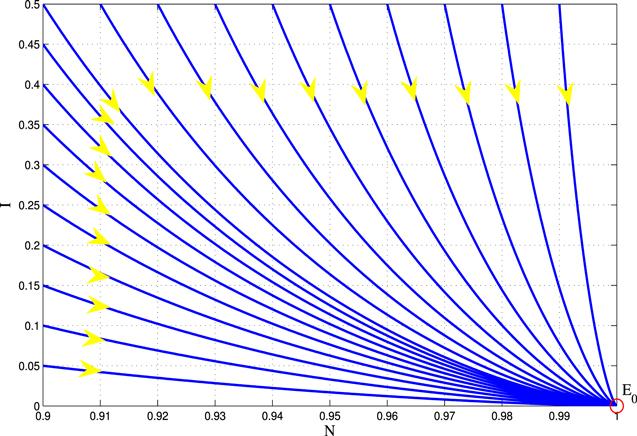
Figure 1. Global dynamics of the model (5) in Case 1 of Example 1.
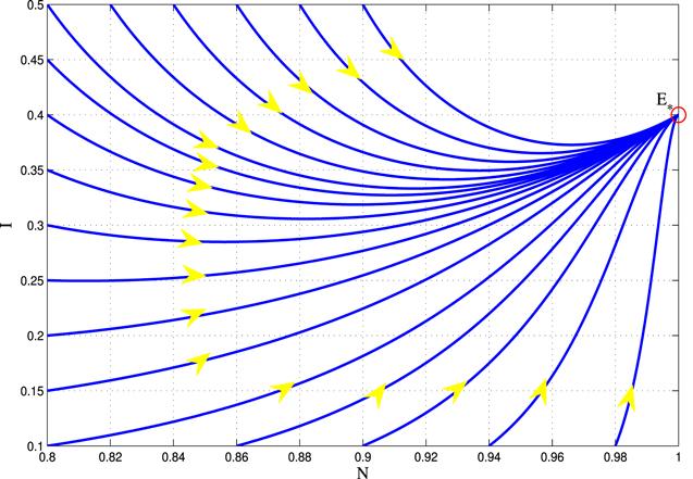
Figure 2. Global dynamics of the model (5) in Case 2 of Example 1.
Table 1. The set of the parameters used in Example 1.
Case b σ β Remark GAS
1 0.25 0.4 0.3 σ + b > β E0 = (1, 0)
2 0.10 0.2 0.5 σ + b < β E* = (1, 0.4)
Table 2. The set of the parameters used in Example 2.
Case a b q σ Remark GAS
1 0.25 0.4 0.5 0.3 a + b + qφ(0) > σ ${{ \mathcal E }}_{0}=(1,0)$
2 0.1 0.2 0.45 0.55 a + b + qφ(0) < σ ${{ \mathcal E }}_{* }=(1,0.2644)$

In this example, we consider the model (15) with a smooth control function given by $\varphi (I)=1-{e}^{-I}$ for $I\geqslant 0$ and the parameters given in Table 2.

Figures 3 and 4 sketch phase planes corresponding to specific initial data of the model (15). It is clear that the GAS of the equilibrium points is confirmed. Hence, the assertions in section 3 are supported.
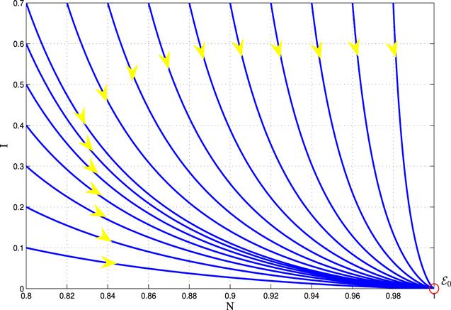
Figure 3. Global dynamics of the model with control strategies (15) in Case 1 of Example 2.
Figure 4. Global dynamics of the model with control strategies (15) in Case 2 of Example 2.

5. Conclusions and discussions

As the first and also the main conclusion of this work, we have provided a rigorous mathematical analysis for the GAS of the compartment models for the spreading of rumors (1) and (2). By using the Lyapunov candidate functions constructed in sections 2 and 3, the complete GAS of the two rumor spreading models has been determined fully. The obtained results in this work improve the ones constructed in [1] and [12].
The GAS analysis of the two rumor spreading models implies that there are only two scenarios of the spreading of the rumors, the first one corresponding to the GAS of the rumor-free equilibrium point means that the rumors will be receded and extinguished and the second one corresponding to the GAS of the rumor-spreading equilibrium point implies that the rumors always appear. Hence, we are able to control the spreading of the rumors by adjusting the parameters in the models. This may be useful in real-world situations.
In recent years, mathematical models described by fractional-order differential equations have been strongly developed and widely used to study complex systems arising in real-world applications, in which the stability problems of fractional-order systems is very important and prominent. The Lyapunov stability theory for fractional-order dynamical systems can be considered as one of the most successful approaches to this problem [26, 2932]. Hence, it is reasonable to assume that the Lyapunov functions proposed in the present work can be utilized to analyze the global dynamics of the rumor spreading models (1) and (2) in the context of fractional-order derivatives. For example, we can consider the Lyapunov candidate functions in sections 2 and 3 with the help of the fractional-order Lyapunov theory in [26, 2932] to study stability properties of the following fractional-order versions
$\begin{eqnarray}\begin{array}{rcl}{}_{0}^{C}{D}_{t}^{\alpha }S & = & \widehat{b}S+(\widehat{b}+\widehat{\sigma })I-\widehat{b}{S}^{2}-(\widehat{\beta }+\widehat{b}){SI},\\ {}_{0}^{C}{D}_{t}^{\alpha }I & = & -\widehat{\sigma }I-\widehat{b}{I}^{2}+(\widehat{\beta }-\widehat{b}){SI},\end{array}\end{eqnarray}$
and
$\begin{eqnarray}\begin{array}{rcl}{}_{0}^{C}{D}_{t}^{\alpha }S & = & \widehat{a}S-\widehat{a}{S}^{2}+(\widehat{a}+\widehat{b})I-(\widehat{\sigma }+\widehat{a}){SI}+\widehat{q}\varphi (I)I,\\ {}_{0}^{C}{D}_{t}^{\alpha }I & = & -\widehat{b}I-\widehat{a}{I}^{2}+(\widehat{\sigma }-\widehat{a}){SI}-\widehat{q}\varphi (I)I,\end{array}\end{eqnarray}$
where ${}_{0}^{C}{D}_{t}^{\alpha }f(t)$ denotes for the Caputo fractional derivative of a given function f(t) (see [33, 34]).
The proposed Lyapunov functions in the present work may be only suitable with the two rumor spreading models under consideration. Hence, it is necessary to propose new Lyapunov function candidates or different approaches to study the stability properties of other rumor spreading models that are more complex in form or structure. This issue will be considered in future studies.
In the near future, we will study stability properties and practical applications of the rumor spreading models (1) and (2) in the context of fractional-order derivative operators. Also, reliable numerical methods for solving the models (1) and (2) as well as their fractional-order versions will be considered.

Ethical approval

Not applicable.

Availability of supporting data

The data supporting the findings of this study are available within the article [and/or] its supplementary materials.

Conflicts of interest

We have no conflicts of interest to disclose.

Funding information

Not available.

Authors' contributions

Manh Tuan Hoang: Conceptualization, Methodology, Software, Formal analysis, Writing- Original draft preparation, Methodology, Writing—Review and Editing, Supervision.

We would like to thank the editor and anonymous referees for useful and valuable comments that led to a great improvement of the paper.

1
Dong S Huang Y-C 2018 A class of rumor spreading models with population dynamics Commun. Theor. Phys. 70 795 802

DOI

2
Guo H Yan X 2023 Dynamic modeling and simulation of rumor propagation based on the double refutation mechanism Inf. Sci. 630 385 402

DOI

3
Hua Y Pan Q Hou W He M 2018 Rumor spreading model considering the proportion of wisemen in the crowd Physica A 505 1084 1094

DOI

4
Jia P Wang C Zhang G Ma J 2019 A rumor spreading model based on two propagation channels in social networks Physica A 524 342 353

DOI

5
Jia F Lv G 2018 Dynamic analysis of a stochastic rumor propagation model Physica A 490 613 623

DOI

6
Ke Y Zhu L Wu P Shi L 2022 Dynamics of a reaction-diffusion rumor propagation model with non-smooth control Appl. Math. Comput. 435 127478

DOI

7
Kishore R Tyagi I Rao Y S Kumar D 2022 Epidemic model on rumor propagation in e-commerce Mater. Today: Proc. 57 2056 2060

DOI

8
Nwaibeh E A Chikwendu C R 2023 A deterministic model of the spread of scam rumor and its numerical simulations Math. Comput. Simul 207 111 129

DOI

9
Piqueira J R C Zilbovicius M Batistela C M 2020 Daley-Kendal models in fake-news scenario Physica A 548 123406

DOI

10
Yu Z Lu S Wang D Li Z 2021 Modeling and analysis of rumor propagation in social networks Inf. Sci. 580 857 873

DOI

11
Zhang Y Zhu J 2019 Dynamic behavior of an I2S2R rumor propagation model on weighted contract networks Physica A 536 120981

DOI

12
Zhu H Zhang X An Q 2022 Global stability of a rumor spreading model with discontinuous control, strategies Physica A 606 128157

DOI

13
Guo H Yin Q Xia C Dehmer M 2021 Impact of information diffusion on epidemic spreading in partially mapping two-layered time-varying networks Nonlinear Dyn. 105 3819 3833

DOI

14
Xia C Wang L Sun S Wang J 2012 An SIR model with infection delay and propagation vector in complex networks Nonlinear Dyn. 69 927 934

DOI

15
Xia C Sun S Rao F Sun J Wang J Chen Z 2009 SIS model of epidemic spreading on dynamical networks with community Front. Comput. Sci. China 3 361 365

DOI

16
Khalil H K 2002 Nonlinear Systems 3rd edn Pearson

17
LaSalle J Lefschetz S 1961 Stability by Liapunov's Direct Method with Applications Academic Press

18
LaSalle J P 1976 The Stability of Dynamical Systems Philadelphia, PA Society for Industrial and Applied Mathematics CBMS-NSF Regional Conference Series in Applied Mathematics

DOI

19
Liapunov A M 1966 Stability of Motion Academic

20
Allen L J S 2007 Introduction to Mathematical Biology Pearson Education, Inc, Prentice Hall

21
Edelstein-Keshet L 2005 Mathematical Models in Biology Philadelphia, PA Society for Industrial and Applied Mathematics

22
Martcheva M 2015 An Introduction to Mathematical Epidemiology Springer

23
Korobeinikov A 2004 Global properties of basic virus dynamics models Bull. Math. Biol. 66 879 883

24
Korobeinikov A 2004 Lyapunov functions and global properties for SEIR and SEIS epidemic models Math. Med. Biol. J. IMA 21 75 83

DOI

25
O'Regan S M Kelly T C Korobeinikov A O'Callaghan M J A Pokrovskii A V 2010 Lyapunov functions for SIR and SIRS epidemic models Appl. Math. Lett. 23 446 448

DOI

26
Vargas-De-León C 2015 Volterra-type Lyapunov functions for fractional-order epidemic systems Commun. Nonlinear Sci. Numer. Simul. 24 75 85

DOI

27
Vargas-De-León C 2011 On the global stability of SIS, SIR and SIRS epidemic models with standard incidence Chaos, Solitons Fractals 44 1106 1110

DOI

28
Ascher U Petzold L 1998 Computer methods for ordinary differential equations and differential-algebraic equations Society for Industrial and Applied Mathematics

29
Agarwal R P O'Regan D Hristova S 2015 Stability of Caputo fractional differential equations by Lyapunov functions Appl. Math. 60 653 676

DOI

30
Aguila-Camacho N Duarte-Mermoud A M Gallegos J A 2014 Lyapunov functions for fractional order systems Commun. Nonlinear Sci. Numer. Simul. 19 2951 2957

DOI

31
Duarte-Mermoud M A Aguila-Camacho N Gallegos J A Castro-Linares R 2015 Using general quadratic Lyapunov functions to prove Lyapunov uniform stability for fractional order systems Commun. Nonlinear Sci. Numer. Simul. 22 650 659

DOI

32
Li Y Chen Y Q Podlubny I 2010 Stability of fractional-order nonlinear dynamic systems: Lyapunov direct method and generalized Mittag-Leffler stability Comput. Math. Appl. 59 1810 1821

DOI

33
Caputo M 1967 Linear models of dissipation whose Q is almost frequency independent-II Geophys. J. Int. 13 529 539

DOI

34
Kilbas A A Srivastava H M Trujillo J J 2006 Theory and Applications of Fractional Differential Equations vol 204 1st edn Elsevier Science, Inc.

Outlines

/