Welcome to visit Communications in Theoretical Physics,
Mathematical Physics

$\bar{\partial }$-dressing method for the complex modified KdV equation

  • Shuxin Yang 1, 2 ,
  • Biao Li , 1
Expand
  • 1School of Mathematics and Statistics, Ningbo University, Ningbo 315211, China
  • 2School of Foundation Studies, Zhejiang Pharmaceutical University, Ningbo 315500, China

Received date: 2023-07-13

  Revised date: 2023-08-16

  Accepted date: 2023-09-27

  Online published: 2023-11-10

Copyright

© 2023 Institute of Theoretical Physics CAS, Chinese Physical Society and IOP Publishing

Abstract

The dressing method based on the 2 × 2 matrix $\bar{\partial }$-problem is generalized to study the complex modified KdV equation (cmKdV). Through two linear constraint equations, the spatial and time spectral problems related to the cmKdV equation are derived. The gauge equivalence between the cmKdV equation and the Heisenberg chain equation is obtained. Using a recursive operator, a hierarchy of cmKdV with source is proposed. On the basis of the $\bar{\partial }$-equation, the N-solition solutions of the cmKdV equation are obtained by selecting the appropriate spectral transformation matrix. Furthermore, we get explicit one-soliton and two-soliton solutions.

Cite this article

Shuxin Yang , Biao Li . $\bar{\partial }$-dressing method for the complex modified KdV equation[J]. Communications in Theoretical Physics, 2023 , 75(11) : 115003 . DOI: 10.1088/1572-9494/acfd8c

1. Introduction

In this paper, we consider the complex modified Korteweg–de Vries equation (cmKdV) [1] as follows:
$\begin{eqnarray}{u}_{t}+{u}_{{xxx}}+6| u{| }^{2}{u}_{x}=0.\end{eqnarray}$
Here, u = u(x, t) is a complex function of x and t. The cmKdV equation is a typical integrable partial differential equation. It has been studied extensively over the last decades and its mathematical properties are well-documented in the literature. For example, the soliton solutions, the breathers and super-regular breathers, the rogue wave solutions, the existence and stability of solitary wave solutions, periodic traveling waves, exact group invariant solutions and conservation laws have been discussed in [111]. On the other hand, it is often suitable for many physical situations, such as the propagation of few-cycle optical pulses in cubic nonlinear media, electromagnetic wave propagation in liquid crystal waveguides and transverse wave propagation in molecular chain models [1217].
The $\bar{\partial }$-dressing method is a powerful tool for constructing and solving integrable nonlinear equations and describing their transformations and reductions. This method was first proposed by Zakharov and Shabat [18], and further developed by Beals, Coifman, Ablowitz, ManBakov, Fokas et al [1924]. So far, a great deal of integrable equations have been widely discussed by the $\bar{\partial }$-dressing method [2533]. However, to our knowledge, there is still no research work on the cmKdV equation (1.1) by using the $\bar{\partial }$-dressing method. In this paper, we use the $\bar{\partial }$-dressing method to study Lax pairs, and cmKdV hierarchy with source and N-soliton solutions of the cmKdV equation (1.1).
The layout of this paper is organized as follows. In section 2, we obtain the Lax pair with singular dispersion relation by using the $\bar{\partial }$-dressing method. In section 3, we introduce a cmKdV hierarchy with source, which contains a cmKdV hierarchy for a special case. In section 4, the N-soliton solutions is constructed. As an application of the N-soliton formula, we discuss one-soliton and two-soliton in section 5. Finally, the conclusions will be drawn based on the above sections.

2. Spectral problem and Lax pair

2.1. The spatial spectral problem

We consider the 2 × 2 matrix $\bar{\partial }$-problem in the complex k-plane
$\begin{eqnarray}\bar{\partial }\psi =\psi R,\end{eqnarray}$
with a boundary condition ψ(x, t, k) → I, k → ∞, then a solution of the equation (2.1) can be written as
$\begin{eqnarray}\psi (k)=I+\displaystyle \frac{1}{2\pi {\rm{i}}}\int \int \displaystyle \frac{\psi (z)R(z)}{z-k}{\rm{d}}z\wedge {\rm{d}}\bar{z}\equiv I+\psi {{RC}}_{k},\end{eqnarray}$
where Ck denotes the Cauchy–Green integral operator acting on the left. The formal solution of $\bar{\partial }$-problem (2.1) will be given from (2.2) as
$\begin{eqnarray}\psi (k)=I\cdot {\left(I-{{RC}}_{k}\right)}^{-1}.\end{eqnarray}$
For convenience, we define a pairing [26]
$\begin{eqnarray*}\begin{array}{rcl}\langle f,g\rangle & = & \displaystyle \frac{1}{2\pi {\rm{i}}}\int \int f(k){g}^{{\rm{T}}}(k){\rm{d}}k\wedge {\rm{d}}\bar{k},\\ \langle f\rangle & = & \langle f,I\rangle =\displaystyle \frac{1}{2\pi {\rm{i}}}\int \int f(k){\rm{d}}k\wedge {\rm{d}}\bar{k},\end{array}\end{eqnarray*}$
which can be shown to possess the following properties
$\begin{eqnarray}\begin{array}{rcl}\langle f,g{\rangle }^{{\rm{T}}} & = & \langle g,f\rangle ,\ \langle {fR},g\rangle =\langle f,{{gR}}^{{\rm{T}}}\rangle ,\\ \langle {{fC}}_{k},g\rangle & = & -\langle f,{{gC}}_{k}\rangle .\end{array}\end{eqnarray}$
It is easy to prove that for some matrix functions f(k) and g(k), the operator Ck satisfies
$\begin{eqnarray}g(k)[f(k){C}_{k}]{C}_{k}+[g(k){C}_{k}]f(k){C}_{k}=[g(k){C}_{k}][f(k){C}_{k}].\end{eqnarray}$
It is well known that the Lax pairs of nonlinear equations play an important role in the study of integrable systems. Such as the Darboux transformation, inverse scattering transformation, Riemann–Hilbert method, and the algebro-geometric method rely on their Lax pairs. Here we prove that if the transform matrix R(x, t, k) satisfies a simple linear equation, the spatial-time spectral problems of the cmkdv equation can be established from (2.1). In particular, we obtain the spatial-time spectral problems of the cmKdV equation.

Let the transform matrix R satisfies

$\begin{eqnarray}{R}_{x}={\rm{i}}k[R,{\sigma }_{3}],\end{eqnarray}$
where ${\sigma }_{3}=\mathrm{diag}(1,-1)$, then the solution ψ of the $\bar{\partial }$-equation (2.1) satisfies the following spatial spectral problem
$\begin{eqnarray}{\psi }_{x}+{\rm{i}}k[{\sigma }_{3},\psi ]=Q\psi ,\end{eqnarray}$
where
$\begin{eqnarray}Q=\left(\begin{array}{cc}0 & q\\ -\bar{q} & 0\end{array}\right)=-{\rm{i}}[{\sigma }_{3},\langle \psi R\rangle ].\end{eqnarray}$

Using (2.3) and (2.6), we get

$\begin{eqnarray}{\psi }_{x}={\rm{i}}k\psi R{\sigma }_{3}{C}_{k}{\left(I-{{RC}}_{k}\right)}^{-1}-{\rm{i}}k\psi {\sigma }_{3}{{RC}}_{k}{\left(I-{{RC}}_{k}\right)}^{-1},\end{eqnarray}$
According to the definition of Ck, we can obtain
$\begin{eqnarray}{\rm{i}}k\psi {{RC}}_{k}={\rm{i}}\langle \psi R\rangle +{\rm{i}}k(\psi -I).\end{eqnarray}$
Since ${{RC}}_{k}=I-I\cdot (I-{{RC}}_{k})$, then we find
$\begin{eqnarray}{{RC}}_{k}{\left(I-{{RC}}_{k}\right)}^{-1}={\left(I-{{RC}}_{k}\right)}^{-1}-I.\end{eqnarray}$
Substituting (2.10) and (2.11) into (2.9), we obtain
$\begin{eqnarray}{\psi }_{x}={\rm{i}}\langle \psi R\rangle {\sigma }_{3}\psi -{\rm{i}}{\sigma }_{3}k{\left(I-{{RC}}_{k}\right)}^{-1}+{\rm{i}}k\psi {\sigma }_{3}.\end{eqnarray}$
From (2.10), we can get
$\begin{eqnarray}k{\left(I-{{RC}}_{k}\right)}^{-1}=\langle \psi R\rangle \psi +k\psi .\end{eqnarray}$
Substituting (2.13) into (2.12), we have equation (2.7).

2.2. The time spectral problem

Suppose that R satisfies the linear equation

$\begin{eqnarray}{R}_{t}=[R,{\rm{\Omega }}],\end{eqnarray}$
where
$\begin{eqnarray}{\rm{\Omega }}={{\rm{\Omega }}}_{p}+{{\rm{\Omega }}}_{s}=4{\rm{i}}{k}^{3}{\sigma }_{3}+\displaystyle \frac{1}{2\pi {\rm{i}}}\int \int \displaystyle \frac{\omega (\xi ){\sigma }_{3}}{\xi -k}{\rm{d}}\xi \wedge {\rm{d}}\bar{\xi },\end{eqnarray}$
which comprises both a polynomial part ${{\rm{\Omega }}}_{p}(k)$ and a singular part ${{\rm{\Omega }}}_{s}(k)$ and $\omega (\xi )$ is a scalar function. Then the solution ψ of the $\bar{\partial }$-equation (2.1) leads to time spectral problem
$\begin{eqnarray}\begin{array}{l}{\psi }_{t}+4{\rm{i}}{k}^{3}[{\sigma }_{3},\psi ]=(2{Q}^{3}+2{\rm{i}}k{\sigma }_{3}{Q}_{x}-2{\rm{i}}{{kQ}}^{2}{\sigma }_{3}\\ \quad +4{k}^{2}Q-{Q}_{{xx}})\psi \\ \quad -\displaystyle \frac{1}{2\pi {\rm{i}}}(\psi {\sigma }_{3}{\psi }^{-1}\omega (k){C}_{k})\psi +\psi {{\rm{\Omega }}}_{s}.\end{array}\end{eqnarray}$

As $\omega (k)=0$, the equation (2.16) reduces to

$\begin{eqnarray}\begin{array}{l}{\psi }_{t}+4{\rm{i}}{k}^{3}[{\sigma }_{3},\psi ]=(2{Q}^{3}+2{\rm{i}}k{\sigma }_{3}{Q}_{x}\\ \quad -2{\rm{i}}{{kQ}}^{2}{\sigma }_{3}+4{k}^{2}Q-{Q}_{{xx}})\psi ,\end{array}\end{eqnarray}$
which together with (2.7) gives the Lax pair of the cmKdV equation (1.1).

We first use the polynomial dispersion relation only ${\rm{\Omega }}={{\rm{\Omega }}}_{p}=4{\rm{i}}{k}^{3}{\sigma }_{3}$. From equations (2.2), (2.3) and (2.15), we arrive that

$\begin{eqnarray}\begin{array}{l}{\psi }_{t}=4{\rm{i}}[{k}^{3}\psi {{RC}}_{k}{\sigma }_{3}{\left(I-{{RC}}_{k}\right)}^{-1}\\ \quad -{k}^{3}\psi {\sigma }_{3}{\left(I-{{RC}}_{k}\right)}^{-1}]+4{\rm{i}}{k}^{3}\psi {\sigma }_{3}.\end{array}\end{eqnarray}$
Through the following direct computation
$\begin{eqnarray}\begin{array}{rcl}k\psi {{RC}}_{k} & = & \langle \psi R\rangle +k(\psi -I),\\ {k}^{2}\psi {{RC}}_{k} & = & \langle k\psi R\rangle +k\langle \psi R\rangle +{k}^{2}(\psi -I),\\ {k}^{3}\psi {{RC}}_{k} & = & \langle {k}^{2}\psi R\rangle +k\langle k\psi R\rangle +{k}^{2}\langle \psi R\rangle +{k}^{3}(\psi -I),\end{array}\end{eqnarray}$
then (2.18) is changed to
$\begin{eqnarray}\begin{array}{rcl}{\psi }_{t} & = & -4{\rm{i}}{k}^{3}[{\sigma }_{3},\psi ]+4{\rm{i}}[\langle {k}^{2}\psi R\rangle ,{\sigma }_{3}]\psi \\ & & +4{\rm{i}}[\langle k\psi R\rangle ,{\sigma }_{3}](k+\langle \psi R\rangle )\psi \\ & & +4{\rm{i}}[\langle \psi R\rangle ,{\sigma }_{3}]({k}^{2}+\langle k\psi R\rangle +k\langle \psi R\rangle +\langle \psi R{\rangle }^{2})\psi .\end{array}\end{eqnarray}$
By using (2.6), (2.7) and (2.8), we obtain
$\begin{eqnarray}\begin{array}{rcl}\langle \psi R{\rangle }_{x} & = & {\rm{i}}[\langle k\psi R\rangle ,{\sigma }_{3}]+Q\langle \psi R\rangle ,\\ \langle k\psi R{\rangle }_{x} & = & {\rm{i}}[\langle {k}^{2}\psi R\rangle ,{\sigma }_{3}]+Q\langle k\psi R\rangle .\end{array}\end{eqnarray}$
Hence, equation (2.20) reduces to
$\begin{eqnarray}\begin{array}{l}{\psi }_{t}+4{\rm{i}}{k}^{3}[{\sigma }_{3},\psi ]=(4\langle k\psi R{\rangle }_{x}+4k\langle \psi R{\rangle }_{x}\\ \quad +4\langle \psi R{\rangle }_{x}\langle \psi R\rangle +4{k}^{2}Q)\psi .\end{array}\end{eqnarray}$
By means of (2.6), (2.7) and (2.8), we have
$\begin{eqnarray}\begin{array}{rcl}\langle k\psi R{\rangle }_{x}^{\mathrm{off}} & = & -\displaystyle \frac{{\rm{i}}}{2}{\sigma }_{3}Q\langle \psi R\rangle +\displaystyle \frac{{\rm{i}}}{2}{\sigma }_{3}\langle \psi R{\rangle }_{x},\\ \langle k\psi R{\rangle }_{x}^{\mathrm{diag}} & = & \displaystyle \frac{{\rm{i}}}{2}{\sigma }_{3}{Q}^{2}\langle \psi R\rangle -\displaystyle \frac{{\rm{i}}}{2}{\sigma }_{3}Q\langle \psi R{\rangle }_{x}.\end{array}\end{eqnarray}$
Substituting (2.23) into (2.22) leads to the time evolution equation
$\begin{eqnarray}\begin{array}{l}{\psi }_{t}+4{\rm{i}}{k}^{3}[{\sigma }_{3},\psi ]=(2{Q}^{3}+2{\rm{i}}k{\sigma }_{3}{Q}_{x}-2{\rm{i}}{{kQ}}^{2}{\sigma }_{3}\\ \quad +4{k}^{2}Q-{Q}_{{xx}})\psi .\end{array}\end{eqnarray}$
In the following, we consider the singular dispersion relation in (2.15). In the same way, we have
$\begin{eqnarray}{\psi }_{t}=(\psi R{{\rm{\Omega }}}_{s}{C}_{k}-\psi {{\rm{\Omega }}}_{s}){\left(I-{{RC}}_{k}\right)}^{-1}+\psi {{\rm{\Omega }}}_{s}.\end{eqnarray}$
And resorting (2.2) and (2.5), $\psi R{{\rm{\Omega }}}_{s}{C}_{k}$ in (2.25) satisfies
$\begin{eqnarray}\psi R{{\rm{\Omega }}}_{s}{C}_{k}=\psi {{\rm{\Omega }}}_{s}-\displaystyle \frac{1}{2\pi {\rm{i}}}\int \int \displaystyle \frac{\omega (\xi )\psi (\xi ){\sigma }_{3}}{\xi -k}{\rm{d}}\xi \wedge {\rm{d}}\bar{\xi }.\end{eqnarray}$
Hence, we have
$\begin{eqnarray}{\psi }_{t}=-\displaystyle \frac{1}{2\pi {\rm{i}}}\int \int \displaystyle \frac{\omega (\xi )\psi (\xi ){\sigma }_{3}}{\xi -k}{\rm{d}}\xi \wedge {\rm{d}}\bar{\xi }{\left(I-{{RC}}_{k}\right)}^{-1}+\psi {{\rm{\Omega }}}_{s}.\end{eqnarray}$
By using the relations
$\begin{eqnarray*}\displaystyle \frac{1}{\rho -k}\displaystyle \frac{1}{\xi -\rho }=\displaystyle \frac{1}{\xi -k}\left(\displaystyle \frac{1}{\rho -k}-\displaystyle \frac{1}{\rho -\xi }\right),\end{eqnarray*}$
we find that
$\begin{eqnarray*}\displaystyle \frac{1}{k-\xi }{\left(I-{{RC}}_{k}\right)}^{-1}=\displaystyle \frac{1}{k-\xi }{\psi }^{-1}(\xi )\psi (k),\end{eqnarray*}$
by which, then (2.27) gives a time-dependent linear equation with the singular dispersion relation
$\begin{eqnarray}{\psi }_{t}=-\displaystyle \frac{1}{2\pi {\rm{i}}}(\psi {\sigma }_{3}{\psi }^{-1}\omega (k){C}_{k})\psi +\psi {{\rm{\Omega }}}_{s},\end{eqnarray}$
which together with (2.24) gives (2.16).

2.3. Gauge equivalence

In this section, we prove that there is a gauge equivalence between the cmKdV equation and the Heisenberg chain equation.

The cmKdV equation (1.1) is gauge equivalent with the Heisenberg chain equation

$\begin{eqnarray}{S}_{t}=-\displaystyle \frac{{\rm{i}}}{2}[S,{S}_{{xx}}],\ \ \ \ {S}^{2}=I.\end{eqnarray}$

Making a reversible transformation $g(x,t)$,

$\begin{eqnarray*}\psi (x,t,k)=g(x,t)\varphi (x,t,k),\ \ \ g(x,t)=\psi (k=0).\end{eqnarray*}$
Then we can calculate that $\varphi (x,t,k)$ satisfies the following $\bar{\partial }$-problem,
$\begin{eqnarray}\bar{\partial }\varphi ={g}^{-1}\psi R=\varphi R,\varphi (k)\to {g}^{-1},k\to \infty .\end{eqnarray}$
The equation (2.30) admits a solution
$\begin{eqnarray}\varphi (k)={g}^{-1}+\displaystyle \frac{1}{2\pi {\rm{i}}}\int \int \displaystyle \frac{\varphi (\zeta )R(\zeta )}{\zeta -k}{\rm{d}}\zeta \wedge {\rm{d}}\bar{\zeta }={g}^{-1}+\varphi {{RC}}_{k}.\end{eqnarray}$
From (2.31), we have
$\begin{eqnarray}\varphi (k)={g}^{-1}{\left(I-{{RC}}_{k}\right)}^{-1}.\end{eqnarray}$
Deriving equation (2.32) with respect to space variable x and using (2.7), we obtain
$\begin{eqnarray}\begin{array}{l}{\varphi }_{x}=-{g}^{-1}{g}_{x}\varphi +{\rm{i}}k\varphi R{\sigma }_{3}{C}_{k}{\left(I-{{RC}}_{k}\right)}^{-1}\\ \quad -{\rm{i}}k\varphi {\sigma }_{3}{{RC}}_{k}{\left(I-{{RC}}_{k}\right)}^{-1}.\end{array}\end{eqnarray}$
Similar to the previous calculation, we can simplify the above formula to
$\begin{eqnarray}{\varphi }_{x}=-{g}^{-1}\{{g}_{x}+{\rm{i}}[{\sigma }_{3},\langle \psi R\rangle ]g\}\varphi -{\rm{i}}{{kg}}^{-1}{\sigma }_{3}g\varphi +{\rm{i}}k\varphi {\sigma }_{3}.\end{eqnarray}$
We can choose the function g to satisfy the following condition
$\begin{eqnarray*}{g}_{x}=-{\rm{i}}[{\sigma }_{3},\langle \psi R\rangle ]g.\end{eqnarray*}$
Let $S={g}^{-1}{\sigma }_{3}g$, then the equation (2.33) gives the spatial–spectral problem
$\begin{eqnarray}{\varphi }_{x}=-{\rm{i}}{kS}\varphi +{\rm{i}}k\varphi {\sigma }_{3}.\end{eqnarray}$
The compatible condition leads to the Heisenberg chain equation
$\begin{eqnarray}{S}_{t}=-\displaystyle \frac{{\rm{i}}}{2}[S,{S}_{{xx}}],\ \ \ \ {S}^{2}=I.\end{eqnarray}$

3. Recursive operators and cmKdV hierarchy

In this section, we derive the cmKdV equation with a source. First of all, we define the matrix M in the following form
$\begin{eqnarray}M=\left(\begin{array}{cc}-r & p\\ \bar{p} & r\end{array}\right)=\psi {\sigma }_{3}{\psi }^{-1}.\end{eqnarray}$
By using (2.8) and (3.1), we can obtain the following proposition.

Q defined by (2.8) satisfies a coupled hierarchy with a source M

$\begin{eqnarray}\begin{array}{ccc}{Q}_{t}+2{\alpha }_{n}{\sigma }_{3}{{\rm{\Lambda }}}^{n}Q & = & {\rm{i}}[{\sigma }_{3},\langle \omega (k)M(k)\rangle ],{\unicode{x000A0}}n=1,2,\ldots \\ {M}_{x}+{\rm{i}}k[{\sigma }_{3},M] & = & [Q,M].\end{array}\end{eqnarray}$

For the special case when $n=2,{\alpha }_{n}=2{\rm{i}}$, the hierarchy (3.2) give the cmKdV equation with source

$\begin{eqnarray}\begin{array}{l}{\rm{i}}{q}_{x}+{q}_{{xx}}+2| q{| }^{2}q=\ll p\gg ,\\ {p}_{x}+2{\rm{i}}{kp}=2{qr},\ {r}_{x}=-(r\bar{p}+\bar{r}p).\end{array}\end{eqnarray}$
where $\ll p\gg =\,\tfrac{1}{2\pi {\rm{i}}}\int \int \omega (\xi )p(\xi ){\rm{d}}\xi \wedge {\rm{d}}\bar{\xi }$, and $\omega (\xi )$ is a scalar function in the singular dispersion relation. By choosing $\omega (\xi )=0$, the equation (3.3) exactly reduces to the cmKdV equation (1.1).

Differentiating the expression of Q with respect to t yields

$\begin{eqnarray}{Q}_{t}=-{\rm{i}}[{\sigma }_{3},\langle \psi R{\rangle }_{t}],\end{eqnarray}$
Because of $\bar{\partial }f(k){C}_{k}=f(k)$, then we have
$\begin{eqnarray}\begin{array}{rcl}{(\psi R)}_{t} & = & \bar{\partial }{\psi }_{t}(k)=\bar{\partial }[I\cdot (I-{{RC}}_{k}{)}_{t}^{-1}]\\ & = & \bar{\partial }[\psi {R}_{t}{\left(I-{{RC}}_{k}\right)}^{-1}]{C}_{k}\\ & = & \psi {R}_{t}{\left(I-{{RC}}_{k}\right)}^{-1}.\end{array}\end{eqnarray}$
By using (3.5), we can obtain
$\begin{eqnarray}\begin{array}{l}{Q}_{t}=-{\rm{i}}[{\sigma }_{3},\langle \psi {R}_{t}{\left(I-{{RC}}_{k}\right)}^{-1},I\rangle ]=\\ \,-\,{\rm{i}}[{\sigma }_{3},\,\langle \psi {R}_{t},I\cdot {\left(I+{R}^{T}{C}_{k}\right)}^{-1}\rangle ].\end{array}\end{eqnarray}$
From the $\bar{\partial }$-equation (2.1), we have
$\begin{eqnarray*}\bar{\partial }{\psi }^{-1}=-R{\psi }^{-1},\end{eqnarray*}$
which leads to
$\begin{eqnarray*}{\left({\psi }^{-1}\right)}^{T}=I\cdot {\left(I+{R}^{T}{C}_{k}\right)}^{-1}.\end{eqnarray*}$
Therefore, using (2.4) and (2.14), equation (3.6) can be simplified to
$\begin{eqnarray}{Q}_{t}=-{\rm{i}}[{\sigma }_{3},\langle (\bar{\partial }\psi ){\rm{\Omega }}{\psi }^{-1}+\psi {\rm{\Omega }}\bar{\partial }{\psi }^{-1}\rangle ].\end{eqnarray}$
Taking into the fact that ${{\rm{\Omega }}}_{p}={\alpha }_{n}{k}^{n}{\sigma }_{3},{\alpha }_{n}=\mathrm{const}$ and ${{\rm{\Omega }}}_{s}\to 0$ as $k\to \infty $, the above equation can be further reduced
$\begin{eqnarray}\begin{array}{rcl}{Q}_{t} & = & -{\rm{i}}[{\sigma }_{3},\langle \psi {\rm{\Omega }}\bar{\partial }{\psi }^{-1}\rangle ]-{\rm{i}}[{\sigma }_{3},\langle (\bar{\partial }\psi ){\rm{\Omega }}{\psi }^{-1}\rangle ]\\ & = & -{\rm{i}}{\alpha }_{n}[{\sigma }_{3},\langle \bar{\partial }({k}^{n}M(k))\rangle ]+{\rm{i}}[{\sigma }_{3},\langle \omega (k)M(k)\rangle ]\\ & = & -2{\rm{i}}{\alpha }_{n}{\sigma }_{3}\langle \bar{\partial }({k}^{n}M{\left(k\right)}^{{\rm{off}}})\rangle +{\rm{i}}[{\sigma }_{3},\langle \omega (k)M(k)\rangle ].\end{array}\end{eqnarray}$
By virtue of the spectral problem (2.7), one can verify that
$\begin{eqnarray}{M}_{x}+{\rm{i}}k[{\sigma }_{3},M]-[Q,M]=0.\end{eqnarray}$
From (3.9), they satisfy the following equations
$\begin{eqnarray}\begin{array}{rcl}{M}_{x}^{\mathrm{diag}} & = & [Q,{M}^{\mathrm{off}}],\\ {M}_{x}^{\mathrm{off}} & = & 2{\rm{i}}k{\sigma }_{3}{M}^{\mathrm{off}}+[Q,{M}^{\mathrm{diag}}],\end{array}\end{eqnarray}$
which lead to
$\begin{eqnarray}\begin{array}{rcl}{M}^{\mathrm{diag}} & = & {\sigma }_{3}+{\partial }_{x}^{-1}[Q,{M}^{\mathrm{off}}],\\ {M}^{\mathrm{off}} & = & -{\rm{i}}{\left({\rm{\Lambda }}-k\right)}^{-1}Q,\end{array}\end{eqnarray}$
where
$\begin{eqnarray*}{\rm{\Lambda }}\cdot =\,\displaystyle \frac{1}{2}{\rm{i}}{\sigma }_{3}({\partial }_{x}\cdot -[Q,{\partial }_{x}^{-1}[Q,\cdot ]]).\end{eqnarray*}$
The operator Λ usually is called as recursion operator. We expand ${\left({\rm{\Lambda }}-k\right)}^{-1}$ in the series
$\begin{eqnarray*}{\left({\rm{\Lambda }}-k\right)}^{-1}=-\displaystyle \sum _{j=1}^{\infty }{k}^{-j}{{\rm{\Lambda }}}^{j-1}.\end{eqnarray*}$
By using $\bar{{\rm{\partial }}}{k}^{n-j}=\pi \delta (k){\delta }_{j,n+1},j\,=\,1,2,\ldots $, we can derive that
$\begin{eqnarray*}\displaystyle \sum _{j=1}^{\infty }\langle \bar{\partial }{k}^{n-j}\rangle {{\rm{\Lambda }}}^{j-1}Q=-{{\rm{\Lambda }}}^{n}Q,\end{eqnarray*}$
Substituting it into (3.8) leads to the equation (3.2).

4. N-soliton solutions of cmKdV equation

In this section, we will derive the N-soliton solutions of the cmKdV equation (1.1).

Suppose that ${k}_{j}$ and ${\bar{k}}_{j}$ are 2N discrete spectrals in complex plane ${\mathbb{C}}$. we choose a spectral transform matrix R as

$\begin{eqnarray}R=\displaystyle \sum _{j=1}^{N}\pi {{\rm{e}}}^{-{\rm{i}}\theta (k){\sigma }_{3}}\left(\begin{array}{cc}0 & -{c}_{j}\delta (k-{k}_{j})\\ {\bar{c}}_{j}\delta (k-{\bar{k}}_{j}) & 0\end{array}\right){{\rm{e}}}^{{\rm{i}}\theta (k){\sigma }_{3}},\end{eqnarray}$
where cj is const and $\theta (k)={kx}+4{k}^{3}t$, then the cmKdV equation (1.1) admits the N-soliton solutions
$\begin{eqnarray}{q}_{N}(x,t)=2{\rm{i}}\displaystyle \frac{\det \ {M}^{\mathrm{aug}}}{\det \ M},\end{eqnarray}$
where ${M}^{\mathrm{aug}}$ is $(N+1)\times (N+1)$ matrices defined by
$\begin{eqnarray*}\begin{array}{ccc}{M}^{{\rm{a}}{\rm{u}}{\rm{g}}} & = & \left(\begin{array}{cc}0 & {\boldsymbol{Y}}\\ {\boldsymbol{B}} & M\end{array}\right),{\boldsymbol{Y}}=({Y}_{1},\cdots ,{Y}_{N}),{\unicode{x000A0}}{Y}_{j}=-{c}_{j}{{\rm{e}}}^{\left.-2{\rm{i}}\theta ({k}_{j}\right)},\\ {\boldsymbol{B}} & = & {\left(1,\cdots ,1\right)}^{{\rm{T}}}.\end{array}\end{eqnarray*}$

Substituting (4.1) into (2.8), yields

$\begin{eqnarray}q(x,t)=-2{\rm{i}}\displaystyle \sum _{j=1}^{N}{c}_{j}{{\rm{e}}}^{-2{\rm{i}}\theta ({k}_{j})}{\psi }_{11}({k}_{j}).\end{eqnarray}$
Substituting (4.1) into $\bar{\partial }$-equation (2.2) and resorting the properties of δ function, we obtain
$\begin{eqnarray}{\psi }_{11}(k)=1+\displaystyle \sum _{j=1}^{N}\displaystyle \frac{\bar{{c}_{j}}}{k-{\bar{k}}_{j}}{{\rm{e}}}^{2{\rm{i}}\theta ({\bar{k}}_{j})}{\psi }_{12}({\bar{k}}_{j}),\end{eqnarray}$
$\begin{eqnarray}{\psi }_{12}(k)=-\displaystyle \sum _{m=1}^{N}\displaystyle \frac{{c}_{m}}{k-{k}_{m}}{{\rm{e}}}^{-2{\rm{i}}\theta ({k}_{m})}{\psi }_{11}({k}_{m}).\end{eqnarray}$
Replacing k in (4.4) with kn, and k in (4.5) with ${\bar{k}}_{j}$, we get a system of linear equation
$\begin{eqnarray}{\psi }_{11}({k}_{n})=1-\displaystyle \sum _{j=1}^{N}\displaystyle \sum _{m=1}^{N}{C}_{j}({k}_{n})\overline{\left.{C}_{m}({k}_{j}\right)}{\psi }_{11}({k}_{m}),{\unicode{x000A0}}n=1,2,\cdots ,N.\end{eqnarray}$
The above equation can be rewritten as
$\begin{eqnarray}M{\left({\psi }_{11}({k}_{1}),\cdots ,{\psi }_{11}({k}_{N})\right)}^{{\rm{T}}}={\left(1,\cdots ,1\right)}^{{\rm{T}}},\end{eqnarray}$
where M is N × N matrices defined by
$\begin{eqnarray*}\begin{array}{rlc}M & = & I+({A}_{n,m}),{\unicode{x000A0}}{\unicode{x000A0}}{A}_{n,m}=\displaystyle \sum _{j=1}^{N}{C}_{j}({k}_{n})\overline{\left.{C}_{m}({k}_{j}\right)},\\ {C}_{j}(k) & = & \displaystyle \frac{{\bar{c}}_{j}}{k-{k}_{j}}{{\rm{e}}}^{\left.2{\rm{i}}\theta ({\bar{k}}_{j}\right)},{\unicode{x000A0}}m,j=1,2,\cdots ,N.\end{array}\end{eqnarray*}$
According to Cramer's rule, the equation has the following solution
$\begin{eqnarray}\psi ({k}_{n})=\displaystyle \frac{det{\unicode{x000A0}}{M}_{n}^{{\rm{a}}{\rm{u}}{\rm{g}}}}{det{\unicode{x000A0}}M},{\unicode{x000A0}}{\unicode{x000A0}}n=1,2,\cdots ,N,\end{eqnarray}$
where
$\begin{eqnarray*}{M}_{n}^{\mathrm{aug}}=({{\boldsymbol{M}}}_{1},\cdots ,{{\boldsymbol{M}}}_{n-1},{\boldsymbol{B}},{{\boldsymbol{M}}}_{n+1},\cdots ,{{\boldsymbol{M}}}_{N}).\end{eqnarray*}$
Finally, substituting (4.8) into (4.3) further simplifies it to (4.2).

5. Application of the N-soliton formula

In the following, we will give the one-soliton and two-soliton solutions for the cmKdV equation (1.1).
▶For N = 1, taking k1 = ξ + iη, the formula (4.2) gives the one-soliton solution of the cmKdV equation (1.1)
$\begin{eqnarray}q=2{\rm{i}}\eta {{\rm{e}}}^{-2{\rm{i}}\xi x+{\rm{i}}\phi }{\rm{sech}} 2\eta (x-\alpha ),\end{eqnarray}$
where α = (− 3ξη + (ξ3 + ω1)/η)t + ξ0, φ = − 2(3ξ2ηη3)t + 2ω2t + φ0. The graphic of the one-soliton solution is shown in figure 1.
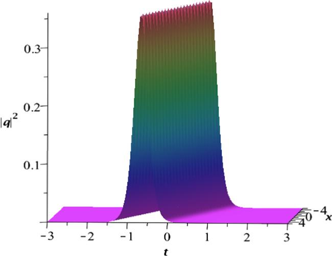
Figure 1. One-soliton solution of equation (1.1) with ξ = 0.2, η = 0.3, ω1 = −2, ω2 = 0.3, ξ0 = φ0 = 0.
▶For N = 2, the formula (4.2) gives the two-soliton solution of the cmKdV equation (1.1) that is given by
$\begin{eqnarray}{q}_{2}=2{\rm{i}}\displaystyle \frac{\det \ {M}^{\mathrm{aug}}}{\det \ M},\end{eqnarray}$
where
$\begin{eqnarray*}\begin{array}{rcl}M & = & \left(\begin{array}{cc}1+{A}_{11} & {A}_{12}\\ {A}_{21} & 1+{A}_{22}\end{array}\right),\\ {M}^{\mathrm{aug}} & = & \left(\begin{array}{ccc}0 & -{c}_{1}{{\rm{e}}}^{-2{\rm{i}}({k}_{1}x+4{k}_{1}^{3}t)} & -{c}_{2}{{\rm{e}}}^{-2{\rm{i}}({k}_{2}x+4{k}_{2}^{3}t)}\\ 1 & 1+{A}_{11} & {A}_{12}\\ 1 & {A}_{21} & 1+{A}_{22}\end{array}\right),\end{array}\end{eqnarray*}$
and
$\begin{eqnarray*}{A}_{i,j}=\displaystyle \frac{{{\rm{\Theta }}}_{1,j}}{-({k}_{i}-{\bar{k}}_{1})({k}_{j}-{\bar{k}}_{1})}+\displaystyle \frac{{{\rm{\Theta }}}_{2,j}}{-({k}_{i}-{\bar{k}}_{2})({k}_{j}-{\bar{k}}_{2})},\end{eqnarray*}$
$\begin{eqnarray*}{\bar{c}}_{i}{c}_{j}={{\rm{e}}}^{{v}_{i}+{v}_{j}},\ {{\rm{\Theta }}}_{i,j}={{\rm{e}}}^{2{\rm{i}}[({\bar{k}}_{i}-{k}_{j})x+4({\bar{k}}_{i}^{3}-{k}_{j}^{3})t]+{v}_{i}+{v}_{j}},\ i,j\,=\,1,2.\end{eqnarray*}$
with vi and vj being two arbitrary constants. The graphic of the two-soliton solution is shown in figure 2.
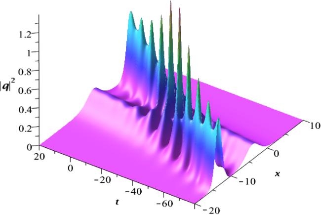
Figure 2. Two-solion solution of equation (1.1) with k1 = −0.1 + 0.2i, k2 = −0.2 + 0.4i, c1 = 1 + 4i, c2 = −1 + i.

6. Conclusion

By means of the $\bar{\partial }$-dressing method, the spatial and time spectral problems associated with the cmKdV equation are obtained. Furthermore, the gauge equivalence between the cmKdV equation and Heisenberg chain equation is obtained. Then a cmKdV hierarchy with source by means of a recursive operator is proposed. Finally, the N-soliton solutions of the cmKdV equation are constructed based on the $\bar{\partial }$-equation by selecting a special spectral transformation matrix. In particular, the explicit one-soliton and two-soliton solutions are discussed.

This work is supported by the National Natural Science Foundation of China (Grant No. 12175111, 11975131), and the KC Wong Magna Fund in Ningbo University.

1
He J 2014 Few-cycle optical rogue waves: complex modified Korteweg-de Vries equation Phys. Rev. E 89 062917

DOI

2
Fan E Lu C 2001 Soliton solutions for the new complex version of a coupled KdV equation and a coupled MKdV equation Phys. Lett. A 285 373 376

DOI

3
Wazwaz A 2005 The tanh and the sine-cosine methods for the complex modified KdV and the generalized KdV equations Comput. Math. Appl. 49 1101 1112

4
Zhaqilao 2013 Nth-order rogue wave solutions of the complex modified Korteweg-de Vries equation Phys. Scr. 87 065401

DOI

5
Liu Y F Guo R Li H 2015 Breathers and localized solutions of complex modified Korteweg-de Vries equation Mod. Phys. Lett. B 29 1550129

DOI

6
Liu C 2017 Superregular breathers in a complex modified Korteweg-de Vries system Chaos 27 083120

DOI

7
Zhidkov E P Iliev I D Kirchev K P 1985 Stability of a solution of the form of a solitary wave for a nonlinear complex modified Korteweg-de Vries equation Siberian Math. J. 26 810 817

8
Hakkaev S Iliev I D Kirchev K 2010 Stability of periodic traveling waves for complex modified Korteweg-de Vries equation J. Differ. Equ. 248 2608 2627

DOI

9
Johnpillai A G Kara A H Biswas A 2013 Invariant solutions and conservation laws of the complex modified korteweg-de vries equation Z. für Naturforsch. A 68 510 514 Exact Group

DOI

10
Ma W X 2021 Nonlocal PT-symmetric integrable equations and related Riemann–Hilbert problems Partial Diff. Equ. Appl. Math. 4 100190

DOI

11
Ma W X 2022 Riemann–Hilbert problems and soliton solutions of type (λ*, −λ*) reduced nonlocal integrable mKdV hierarchies Mathematics 10 870

DOI

12
Leblond H 2012 Circularly polarized few-optical-cycle solitons in Kerr media: a complex modified Korteweg-de Vries model Opt. Commun. 285 356 363

DOI

13
Leblond H Mihalache D 2011 Optical solitons in the few-cycle regime: recent theoretical results Rom. Rep. Phys. 63 1254 1266 ​https://univ-angers.hal.science/hal-03187691

14
Erbay S Şuhubi E S 1989 Nonlinear wave propagation in micropolar media: I. The general theory Int. J. Eng. Sci. 27 895 914

DOI

15
Reyes J A Palffy-Muhoray P 1998 Nonlinear Schrödinger equation in nematic liquid crystals Phys. Rev. E 58 5855 5859

DOI

16
Rodríguez R 2003 Standard and embedded solitons in nematic optical fibers Phys. Rev. E 68 36606 36606

DOI

17
Gorbacheva O B Ostrovsky L A 1983 Nonlinear vector waves in a mechanical model of a molecular chain Physica D 8 223 228

DOI

18
Zakharov V E Shabat A B 1974 A scheme for integrating the nonlinear equations of mathematical physics by the method of the inverse scattering problem: I Funct. Anal. Appl. 8 226 235

19
Ablowitz M J 1983 On the inverse scattering transform for the Kadomtsev–Petviashvili equation Stud. Appl. Math. 69 135 142

DOI

20
Beals R Coifman R R 1986 The D-bar approach to inverse scattering and nonlinear evolutions Physica D 18 242 249

DOI

21
Beals R Coifman R R 1981 Scattering, spectral transformations and nonlinear evolution equations Goulaouic-Meyer-Schwartz 22

22
Fokas A S Santini P M 1990 Dromions and a boundary value problem for the Davey–Stewartson I equation Physica D 44 99 130

DOI

23
Manakov S V 1981 The inverse scattering transform for the time-dependent Schrödinger equation and Kadomtsev–Petviashvili equation Physica D 3 420 427

DOI

24
Zakharov V E Manakov S V 1985 Construction of multidimensional nonlinear integrable systems and their solutions Funkc. Anal. Prilozh. 19 11 25

25
Bogdanov L V Manakov S V 1988 The nonlocal $\bar{\partial }$-problem and (2+1)-dimensional soliton equations J. Phys. A 21 537

26
Doktorov E V Leble S B 2007 A Dressing Method in Mathematical Physics Springer

27
Fokas A S Zakharov V E 1992 The dressing method and nonlocal Riemann–Hilbert problem J. Nonlinear Sci. 2 109 134

DOI

28
Kuang Y K Zhu J Y 2015 A three-wave interaction model with self-consistent sources: the $\bar{\partial }$-dressing method and solutions J. Math. Anal. Appl. 426 783 793

DOI

29
Zhu J Y Geng X G 2014 The AB equations and the $\bar{\partial }$-dressing method in semi-characteristic coordinates Math. Phys. Anal. Geom. 17 49 65

DOI

30
Luo J H Fan E G 2020 $\bar{\partial }$-dressing method for the coupled Gerdjikov–Ivanov equation Appl. Math. Lett. 110 06589

DOI

31
Luo J H Fan E G 2021 Dbar-dressing method for the Gerdjikov–Ivanov equation with nonzero boundary conditions Appl. Math. Lett. 120 107297

DOI

32
Luo J H E G Fan 2021 A $\bar{\partial }$-dressing approach to the Kundu–Eckhaus equation J. Geom. Phys. 167 104291

DOI

33
Yang S X Li B 2023 $\bar{\partial }$-dressing method for the (2+1)-dimensional Korteweg-de Vries equation Appl. Math. Lett. 140 108589

DOI

Outlines

/