Welcome to visit Communications in Theoretical Physics,
Mathematical Physics

The residual symmetry, Bäcklund transformations, CRE integrability and interaction solutions: (2+1)-dimensional Chaffee–Infante equation

  • Nursena Günhan Ay , 1, 2 ,
  • Emrullah Yaşar , 2, *
Expand
  • 1Department of Mathematics, Faculty of Engineering and Natural Sciences, İstanbul Medeniyet University, 34700 Üsküdar, Istanbul, Turkey
  • 2Department of Mathematics, Faculty of Arts and Sciences, Uludag University, 16059 Bursa, Turkey

*Author to whom all correspondence should be addressed.

Received date: 2023-06-05

  Revised date: 2023-08-10

  Accepted date: 2023-09-12

  Online published: 2023-11-10

Copyright

© 2023 Institute of Theoretical Physics CAS, Chinese Physical Society and IOP Publishing

Abstract

In this paper, we consider the (2+1)-dimensional Chaffee–Infante equation, which occurs in the fields of fluid dynamics, high-energy physics, electronic science etc. We build Bäcklund transformations and residual symmetries in nonlocal structure using the Painlevé truncated expansion approach. We use a prolonged system to localize these symmetries and establish the associated one-parameter Lie transformation group. In this transformation group, we deliver new exact solution profiles via the combination of various simple (seed and tangent hyperbolic form) exact solution structures. In this manner, we acquire an infinite amount of exact solution forms methodically. Furthermore, we demonstrate that the model may be integrated in terms of consistent Riccati expansion. Using the Maple symbolic program, we derive the exact solution forms of solitary-wave and soliton-cnoidal interaction. Through 3D and 2D illustrations, we observe the dynamic analysis of the acquired solution forms.

Cite this article

Nursena Günhan Ay , Emrullah Yaşar . The residual symmetry, Bäcklund transformations, CRE integrability and interaction solutions: (2+1)-dimensional Chaffee–Infante equation[J]. Communications in Theoretical Physics, 2023 , 75(11) : 115004 . DOI: 10.1088/1572-9494/acf8b6

1. Introduction

Nature's attractive nonlinearity is the most crucial constraint to comprehending it at its most fundamental level. This approach is widely accepted by researchers. The study of many types of nonlinear ordinary and partial differential equations (PDEs) is essential in the mathematical modeling of complicated systems that fluctuate over time. Physical and natural sciences, neurophysics, population ecology, economics, biomathematics, chemistry, diffusion, biology, heat, and general relativity are all used to develop these models.
Nonlinear evolution equations (NLEEs) can describe many nonlinear physical occurrences in applied science and technology. As a result, finding the exact solutions to the relevant NLEEs is critical for enhancing our understanding of nonlinear events and applying them to practical issues. Therefore, numerous studies have been carried out on this subject [17]. Many ways for achieving exact solutions to NLEEs have been proposed for example Lie symmetry analysis [8, 9], Hirota's method [1012], simplified Hirota's method [3, 13], extended tanh method [14] and numerous other techniques [15, 16]. Some studies to help us understand complex nonlinear wave models, including (2+1) dimensional nonlinear models it is known very recently that N-soliton solutions have been systematically studied by the Hirota bilinear method [12] and by Riemann–Hilbert problems, particularly for higher-order integrable equations [6, 7]. Furthermore, when it comes to symmetry analysis, the approach plays a significant role in analyzing the properties of PDEs [1721]. Nonclassical symmetry [22], Lie-Bäcklund symmetry [23], and nonlocal symmetry [20] have all been extended from classical Lie symmetries.
Finding the nonlocal symmetries of PDEs is a curious issue. Nonlocal symmetries can give rise to new solutions that Lie point symmetries can not produce [17]. The work of [24] presented an approach based on conservation rules for generating nonlocally linked systems in order to achieve nonlocal symmetries. Nonlocal symmetries and nonlocal conservation rules can be investigated by examining nonlocally connected systems [17]. New approaches for building nonlocal symmetry theory and producing nonlocal symmetries have been presented over time. Nonlocal symmetries can be generated using methods such as the Darboux transformation [25, 26], the Bäcklund transformation [27], and the Lax pairs [26, 28]. The Painlevé analysis approach, [17, 29, 30] is a suitable proposed way for revealing the integrability features of PDEs. The truncated Painlevé expansion may be used to build nonlocal symmetries, as presented in [31]. Because they are remnants of the truncated Painlevé expansion, such nonlocal symmetries are now known as residual symmetries [17]. After examining several interaction solutions created by non-local symmetry reduction analysis, the consistent Riccati expansion (CRE) approach [32] was presented to investigate interactions between the soliton and other waveforms When the CRE technique is used for an integrable equation, it is considered CRE solvable.
One of the aforementioned NLEEs is the Chaffe-Infante model. Suppose that the substance diffuses in a region with concentration u(x, y, z). If ϱ(x, y, z, t) is the diffusion coefficient, then
$\begin{eqnarray}{\rm{d}}m=-\varrho \displaystyle \frac{\partial u}{\partial n}{\rm{d}}s{\rm{d}}t\end{eqnarray}$
follows from the diffusion law, where m indicates the amount of diffusion material and ϱ > 0. Equation (1) and the law of conservation of mass produce
$\begin{eqnarray}\begin{array}{l}m={\int }_{{t}_{1}}^{{t}_{2}}\left[{\iint }_{\sum }\varrho \displaystyle \frac{\partial u}{\partial n}{\rm{d}}s\right]{\rm{d}}t={\iiint }_{{\rm{\Omega }}}[u(x,y,z,{t}_{2})\\ \quad -u(x,y,z,{t}_{1})]{\rm{d}}x{\rm{d}}y{\rm{d}}z,\end{array}\end{eqnarray}$
which is
$\begin{eqnarray}\displaystyle \frac{\partial }{\partial x}\left(\varrho \displaystyle \frac{\partial u}{\partial x}\right)+\displaystyle \frac{\partial }{\partial x}\left(\displaystyle \frac{\partial u}{\partial y}\right)+\displaystyle \frac{\partial }{\partial z}\left(\varrho \displaystyle \frac{\partial u}{\partial x}\right)=\displaystyle \frac{\partial u}{\partial t}.\end{eqnarray}$
Take ϱ = 1 and that the influential factor is g(u) = u3u. We achieve
$\begin{eqnarray}\displaystyle \frac{\partial u}{\partial t}=\displaystyle \frac{{\partial }^{2}u}{\partial {x}^{2}}+\displaystyle \frac{{\partial }^{2}u}{\partial {y}^{2}}+\displaystyle \frac{{\partial }^{2}u}{\partial {z}^{2}}+{\rm{\Gamma }}\times (u-{u}^{3}),\end{eqnarray}$
where the variable Γ governs the proportional balance of the diffusion and non-linear elements. Hence the (1 + 1)-dimensional Chaffee–Infante equation is [33]
$\begin{eqnarray}{u}_{t}={u}_{{xx}}+{\rm{\Gamma }}\times (u-{u}^{3}).\end{eqnarray}$
In this paper, we will look at the (2+1)-dimensional Chaffee–Infante equation (CI), which can be produced in the same way as the above. The (CI) equation [34]
$\begin{eqnarray}3\alpha {u}^{2}{u}_{x}-\alpha {u}_{x}+\sigma {u}_{{yy}}+{u}_{{tx}}-{u}_{{xxx}}=0\end{eqnarray}$
(where α is the coefficient of diffusion and σ is the degradation coefficient) is a popular reaction-diffusion model that explains the physical processes of mass transfer and particle diffusion. It is also necessary to have a field of usage in fluid dynamics, electronic science, and many other fields of science. Another feature that makes the CI equation important is that it is the typical model of infinite-dimensional gradient systems, where the structure of the spherical attractor can be fully explained. Here, bifurcation in a system parameter that indicates the potential's steepness also increases the model's attractiveness [35]. The CI equation has been studied using the modified Khater method [35], Lie symmetry analysis [36], the first integral method [37], and a variety of other approaches [38, 39].
The following is how the paper is organized. Using the truncated Painlevé expansion, we derive the Bäcklund transformation and the residual symmetry of equation (6). To locate the residual symmetry to the localized Lie point symmetry, an expanded system of equation (6) is developed. New solutions are obtained with the help of any seed solution in section 2. In the next section, we study the CRE solvability of equation (6). In section 4 we examine the solitary wave profile and interactions profile of equation (6). In the last section we give some conclusions.

2. Residual symmetry and Bäcklund transformation

In this section, we will derive the residual symmetry of equation (6) using the truncated Painlevé expansion. Due to truncated Painlevé analysis solution of equation (6) is expressed as
$\begin{eqnarray}u={u}_{0}+\displaystyle \frac{{u}_{1}}{f},\end{eqnarray}$
where u0 = u0(x, y, t), u1 = u1(x, y, t), and f = f(x, y, t) [17]. Substituting equation (7) into equation (6) and eliminating all of the powers of $\displaystyle \frac{1}{f}$ provides us with;
$\begin{eqnarray}{u}_{0}=\displaystyle \frac{\left({f}_{y}^{2}\sigma -3{f}_{{xx}}{f}_{x}+{f}_{t}{f}_{x}\right)\sqrt{2}}{6\sqrt{\alpha }\ {f}_{x}^{2}},{u}_{1}=\displaystyle \frac{\sqrt{2}\ {f}_{x}}{\sqrt{\alpha }},\end{eqnarray}$
where f holds,
$\begin{eqnarray}\begin{array}{l}\sigma {{PP}}_{x,x}+\sigma {P}_{x,y}+{Q}_{x,x}+\sigma {P}_{x}^{2}+\displaystyle \frac{2\left({\sigma }^{2}{P}^{3}+\sigma {PQ}\right){P}_{x}}{3}\\ \quad +\displaystyle \frac{\left(\sigma {P}^{2}+Q\right){Q}_{x}}{3}-{R}_{x}=0\end{array}\end{eqnarray}$
with Schwarzian variables
$\begin{eqnarray*}P=\displaystyle \frac{{f}_{y}}{{f}_{x}},Q=\displaystyle \frac{{f}_{t}}{{f}_{x}},R=\displaystyle \frac{{f}_{{xxx}}}{{f}_{x}}-\displaystyle \frac{3}{2}\displaystyle \frac{{f}_{{xx}}^{2}}{{f}_{x}^{2}}.\end{eqnarray*}$
We can propose the following Bäcklund-type theorem for equation (6) depending on the Schwarzian form.

If function f is a solution of equation (9), then

$\begin{eqnarray}u=\displaystyle \frac{\left({f}_{y}^{2}\sigma -3{f}_{{xx}}{f}_{x}+{f}_{t}{f}_{x}\right)\sqrt{2}}{6\sqrt{\alpha }\ {f}_{x}^{2}}+\displaystyle \frac{\tfrac{\sqrt{2}\ {f}_{x}}{\sqrt{\alpha }}}{f}\end{eqnarray}$
is a solution of equation (6). According to nonlocal symmetry theory [17, 31] residual symmetry of equation (6) is given by;
$\begin{eqnarray}{\theta }^{u}=\displaystyle \frac{\sqrt{2}\ {f}_{x}}{\sqrt{\alpha }}.\end{eqnarray}$
We know that equation (9) is invariant under the Möbius transformation [17];
$\begin{eqnarray}f\to \displaystyle \frac{k+{lf}}{m+{nf}},({kn}\ne {lm})\end{eqnarray}$
which indicates that f has the point symmetry, taking k = 0, $l=m=1$, $n=\epsilon $
$\begin{eqnarray}{\theta }^{f}=-{f}^{2}.\end{eqnarray}$
The transformation
$\begin{eqnarray}u=\displaystyle \frac{\left({f}_{y}^{2}\sigma -3{f}_{{xx}}{f}_{x}+{f}_{t}{f}_{x}\right)\sqrt{2}}{6\sqrt{\alpha }\ {f}_{x}^{2}}\end{eqnarray}$
may transform equation (6) into equation (9). To ascertain the residual symmetry group
$\begin{eqnarray}u\to \breve{u}=u+\epsilon {\theta }^{u}\end{eqnarray}$
we must solve the initial value problem given below:
$\begin{eqnarray}\displaystyle \frac{{\rm{d}}\breve{u}(\epsilon )}{{\rm{d}}\epsilon }=\displaystyle \frac{\sqrt{2}\ \breve{u}{\left(\epsilon \right)}_{x}}{\sqrt{\alpha }},\breve{u}(\epsilon ){| }_{\epsilon =0}=u.\end{eqnarray}$
Here infinitesimal parameter is denoted by ε. We can see here that the solution to equation (16) can not be found. To easily solve the preceding initial value problem, given an expanded system, one can localize the nonlocal symmetry to the localized Lie point symmetry. As a result, the new variables listed below are necessary
$\begin{eqnarray}{{\rm{\Upsilon }}}_{1}={f}_{x},{{\rm{\Upsilon }}}_{2}={f}_{y},{{\rm{\Upsilon }}}_{3}={f}_{t},{{\rm{\Upsilon }}}_{4}={{\rm{\Upsilon }}}_{1x}.\end{eqnarray}$
Hence we get a prolonged system including (6), (9), (11), and (14). The prolonged system has Lie point symmetry as;
$\begin{eqnarray*}\left(\begin{array}{c}{\theta }^{u}\\ {\theta }^{f}\\ {\theta }^{{{\rm{\Upsilon }}}_{1}}\\ {\theta }^{{{\rm{\Upsilon }}}_{2}}\\ {\theta }^{{{\rm{\Upsilon }}}_{3}}\\ {\theta }^{{{\rm{\Upsilon }}}_{4}}\end{array}\right)=\left(\begin{array}{c}\sqrt{\displaystyle \frac{2}{\alpha }}{{\rm{\Upsilon }}}_{1}\\ -{f}^{2}\\ -2f{{\rm{\Upsilon }}}_{1}\\ -2f{{\rm{\Upsilon }}}_{2}\\ -2f{{\rm{\Upsilon }}}_{3}\\ -2{h}_{1}^{2}-2{{fh}}_{4}\end{array}\right)\end{eqnarray*}$
Due to Lie's first theorem [18, 40], the corresponding initial value problem of Lie point symmetry reads
$\begin{eqnarray*}\displaystyle \frac{{\rm{d}}\breve{u}(\epsilon )}{{\rm{d}}\epsilon }=\sqrt{\displaystyle \frac{2}{\alpha }}\breve{{{\rm{\Upsilon }}}_{1}(\epsilon )},\breve{u}(0)=u,\end{eqnarray*}$
$\begin{eqnarray*}\displaystyle \frac{{\rm{d}}\breve{f}(\epsilon )}{{\rm{d}}\epsilon }=-{\breve{f}}^{2}(\epsilon ),\breve{f}(0)=f,\end{eqnarray*}$
$\begin{eqnarray}\displaystyle \frac{{\rm{d}}\breve{{{\rm{\Upsilon }}}_{1}}(\epsilon )}{{\rm{d}}\epsilon }=-2\breve{f}(\epsilon )\breve{{{\rm{\Upsilon }}}_{1}}(\epsilon ),\breve{{{\rm{\Upsilon }}}_{1}}(0)={{\rm{\Upsilon }}}_{1},\end{eqnarray}$
$\begin{eqnarray*}\displaystyle \frac{{\rm{d}}\breve{{{\rm{\Upsilon }}}_{2}}(\epsilon )}{{\rm{d}}\epsilon }=-2\breve{f}(\epsilon )\breve{{{\rm{\Upsilon }}}_{2}}(\epsilon ),\breve{{{\rm{\Upsilon }}}_{2}}(0)={{\rm{\Upsilon }}}_{2},\end{eqnarray*}$
$\begin{eqnarray*}\displaystyle \frac{{\rm{d}}\breve{{{\rm{\Upsilon }}}_{3}}(\epsilon )}{{\rm{d}}\epsilon }=-2\breve{f}(\epsilon )\breve{{{\rm{\Upsilon }}}_{3}}(\epsilon ),\breve{{{\rm{\Upsilon }}}_{3}}(0)={{\rm{\Upsilon }}}_{3},\end{eqnarray*}$
$\begin{eqnarray*}\displaystyle \frac{{\rm{d}}\breve{{{\rm{\Upsilon }}}_{4}}(\epsilon )}{{\rm{d}}\epsilon }=-2\breve{{{\rm{\Upsilon }}}_{1}}{\left(\epsilon \right)}^{2}-2\breve{f}(\epsilon )\breve{{{\rm{\Upsilon }}}_{4}}(\epsilon ),\breve{{{\rm{\Upsilon }}}_{4}}(0)={{\rm{\Upsilon }}}_{4}.\end{eqnarray*}$
Solving initial value problem given in equation (18) we yield
$\begin{eqnarray}\begin{array}{rcl}\breve{f} & = & \displaystyle \frac{f}{1+\epsilon f},\breve{{{\rm{\Upsilon }}}_{1}}=\displaystyle \frac{{{\rm{\Upsilon }}}_{1}}{{\left(1+\epsilon f\right)}^{2}},\breve{{{\rm{\Upsilon }}}_{2}}=\displaystyle \frac{{{\rm{\Upsilon }}}_{2}}{{\left(1+\epsilon f\right)}^{2}},\\ \breve{{{\rm{\Upsilon }}}_{3}} & = & \displaystyle \frac{{{\rm{\Upsilon }}}_{3}}{{\left(1+\epsilon f\right)}^{2}},\breve{{{\rm{\Upsilon }}}_{4}}=\displaystyle \frac{f\epsilon {{\rm{\Upsilon }}}_{4}-2\epsilon {{\rm{\Upsilon }}}_{1}^{2}+{{\rm{\Upsilon }}}_{4}}{{\left(1+\epsilon f\right)}^{3}}\mathrm{and}\\ \breve{u} & = & u+\displaystyle \frac{\sqrt{2}\,\epsilon {{\rm{\Upsilon }}}_{1}}{\sqrt{\alpha }\left(1+\epsilon f\right)},\end{array}\end{eqnarray}$
where ε is an arbitrary parameter. With the theorem we will provide, we will now assert that it is possible to generate a new solution from an existing one.

If u, f, ${{\rm{\Upsilon }}}_{1}$, ${{\rm{\Upsilon }}}_{2}$, ${{\rm{\Upsilon }}}_{3}$, ${{\rm{\Upsilon }}}_{4}$ is a solution of the prolonged system including (6), (9), (11), (14), then $\breve{u}$, $\breve{f}$, $\breve{{{\rm{\Upsilon }}}_{1}}$, $\breve{{{\rm{\Upsilon }}}_{2}}$, $\breve{{{\rm{\Upsilon }}}_{3}}$, $\breve{{{\rm{\Upsilon }}}_{4}}$ is also the solution of the prolonged system including (6), (9), (11), (14) where

$\begin{eqnarray}\begin{array}{rcl}\breve{f} & = & \displaystyle \frac{f}{1+\epsilon f},\breve{{{\rm{\Upsilon }}}_{1}}=\displaystyle \frac{\breve{{{\rm{\Upsilon }}}_{1}}}{{\left(1+\epsilon f\right)}^{2}},\breve{{{\rm{\Upsilon }}}_{2}}=\displaystyle \frac{\breve{{{\rm{\Upsilon }}}_{2}}}{{\left(1+\epsilon f\right)}^{2}},\\ \breve{{{\rm{\Upsilon }}}_{3}} & = & \displaystyle \frac{\breve{{{\rm{\Upsilon }}}_{3}}}{{\left(1+\epsilon f\right)}^{2}},\breve{{{\rm{\Upsilon }}}_{4}}=\displaystyle \frac{f\epsilon \breve{{{\rm{\Upsilon }}}_{4}}-2\epsilon {\breve{{{\rm{\Upsilon }}}_{1}}}^{2}+\breve{{{\rm{\Upsilon }}}_{4}}}{{\left(1+\epsilon f\right)}^{3}}\\ \breve{u} & = & u+\displaystyle \frac{\sqrt{2}\,\epsilon {{\rm{\Upsilon }}}_{1}}{\sqrt{\alpha }\left(1+\epsilon f\right)}.\end{array}\end{eqnarray}$
Using the finite symmetry transformation given above, one can obtain a new solution from any seed solution of equation (6) and equation (9).

$f={{\rm{e}}}^{{kx}+{ly}+{mt}}$ is a solution of equation (9) with $\alpha =\tfrac{+3{k}^{6}+{l}^{4}{\sigma }^{2}+2k\,{l}^{2}m\sigma +{k}^{2}{m}^{2}}{6{k}^{4}}$ then

$\begin{eqnarray*}u(x,y,t)=\displaystyle \frac{\left(-3{k}^{3}+{l}^{2}\sigma +{km}\right)\sqrt{3}}{3\sqrt{6\alpha }\,{k}^{2}}\end{eqnarray*}$
is a solution of equation (6). By using (20), a new solution of equation (6) is expressed as
$\begin{eqnarray}{u}_{1}(x,y,t)=\displaystyle \frac{\left(\epsilon A{{\rm{e}}}^{{kx}+{ly}+{mt}}-{k}^{3}+\tfrac{{l}^{2}\sigma }{3}+\tfrac{{km}}{3}\right)\sqrt{3}}{\sqrt{6\alpha }\,{k}^{2}\left(1+\epsilon {{\rm{e}}}^{{kx}+{ly}+{mt}}\right)}.\end{eqnarray}$
where $A=\left({k}^{3}+\tfrac{1}{3}{l}^{2}\sigma +\tfrac{1}{3}{km}\right)$.

$f=\tanh \left({kx}+{ly}+{mt}\right)$ is a solution of equation (9) then

$\begin{eqnarray*}u(x,y,t)=\displaystyle \frac{\sqrt{2}\left(6{k}^{3}\tanh \left({kx}+{ly}+{mt}\right)+{l}^{2}\sigma +{mk}\right)}{6\sqrt{\alpha }\,{k}^{2}}\end{eqnarray*}$
is a solution of equation (6) via equation (14) with $\alpha =-\tfrac{-12{k}^{6}-{l}^{4}{\sigma }^{2}-2k\,{l}^{2}m\sigma -{k}^{2}{m}^{2}}{6{k}^{4}}$. By using (20) we obtain a new solution of equation (6) as
$\begin{eqnarray}{u}_{2}(x,y,t)=\displaystyle \frac{2\sqrt{3}\left(\left(\epsilon {S}_{2}+{S}_{1}\right){k}^{3}+\tfrac{m\left({S}_{1}\epsilon +{S}_{2}\right)k}{6}+\tfrac{{l}^{2}\sigma \left({S}_{1}\epsilon +{S}_{2}\right)}{6}\right)}{\sqrt{{\rm{\Psi }}}\,{k}^{2}\left({S}_{1}\epsilon +{S}_{2}\right)},\end{eqnarray}$
where ${S}_{1}=\sinh \left({kx}+{ly}+{mt}\right)$, ${S}_{2}={\rm{\cosh }}({kx}+{ly}+{mt})$ and ${\rm{\Psi }}=\tfrac{12{k}^{6}+{l}^{4}{\sigma }^{2}+2k\,{l}^{2}m\sigma +{k}^{2}{m}^{2}}{{k}^{4}}$ (ε is arbitrary constants).

3. CRE solvability

According to the CRE method [17, 32] the solution of equation (6) is written as
$\begin{eqnarray}u={u}_{0}+{u}_{1}R(w),\end{eqnarray}$
where u0 = u0(x, y, t), u1 = u1(x, y, t) and R(w) is a solution of
$\begin{eqnarray}R{\left(w\right)}_{w}={s}_{0}+{s}_{1}R(w)+{s}_{2}R{\left(w\right)}^{2}.\end{eqnarray}$
Riccati equation with s0, s1 and s2 are arbitrary constants. Plugging equations (23) with (24) into (6) and collecting all the coefficients of the powers of R(w) results in a system of PDEs around u0, and u1. Solving this overdetermined system we get
$\begin{eqnarray}\begin{array}{rcl}{u}_{0} & = & \displaystyle \frac{\sqrt{2}\left(3{\left({w}_{x}\right)}^{3}{s}_{1}-{\left({w}_{y}\right)}^{2}\sigma +3\left({w}_{x}\right)\left({w}_{{xx}}\right)-\left({w}_{x}\right)\left({w}_{t}\right)\right)}{6\sqrt{\alpha }{\left({w}_{x}\right)}^{2}},\\ {u}_{1} & = & \displaystyle \frac{\sqrt{2}\,{s}_{2}\left({w}_{x}\right)}{\sqrt{\alpha }}\end{array}\end{eqnarray}$
and w satisfy
$\begin{eqnarray}\begin{array}{l}6{w}_{{xxxx}}{w}_{x}^{4}=3\kappa {s}_{1}{w}_{x}^{8}+3\left(3\kappa {w}_{{xx}}-2{s}_{1}\alpha \right){w}_{x}^{6}\\ \quad +6{s}_{1}\left(\sigma {w}_{{yy}}+{w}_{{xt}}-{w}_{{xxx}}\right){w}_{x}^{5}\\ \quad +\left(9{s}_{1}{w}_{{xx}}^{2}+6\left(-{s}_{1}{w}_{t}-\alpha \right){w}_{{xx}}+{s}_{1}{w}_{t}^{2}\right.\\ \quad \left.+6{w}_{{xyy}}\sigma +6{w}_{{xxt}}\right){w}_{x}^{4}\\ \quad -6\left({w}_{t}-3{w}_{{xx}}\right)\left(-\displaystyle \frac{{s}_{1}\sigma {w}_{y}^{2}}{3}+{w}_{{xxx}}-\displaystyle \frac{{w}_{{xt}}}{3}\right){w}_{x}^{3}\\ \quad \left(-9{w}_{{xx}}^{3}+6{w}_{t}{w}_{{xx}}^{2}+\left(-12\sigma {w}_{{xy}}{w}_{y}-{w}_{t}^{2}\right){w}_{{xx}}\right.\\ \quad \left.+4\left(\displaystyle \frac{{s}_{1}\sigma {w}_{y}^{3}}{4}+\displaystyle \frac{\left(-3{w}_{{xxx}}+{w}_{{xt}}\right){w}_{y}}{2}+{w}_{{xy}}{w}_{t}\right){w}_{y}\sigma \right){w}_{x}^{2}\\ \quad +4\sigma {w}_{y}^{2}\left(\sigma {w}_{{xy}}{w}_{y}-{w}_{t}{w}_{{xx}}+3{w}_{{xx}}^{2}\right){w}_{x}-3{\sigma }^{2}{w}_{{xx}}{w}_{y}^{4}\end{array}\end{eqnarray}$
where $\kappa ={s}_{1}^{2}-4{s}_{0}{s}_{2}$.
Hence, equation (6) obviously has the truncated Painlevé expansion solution connected to the Riccati equation equation (24). As a result, we can deduce that the equation (6) is CRE solvable [17, 32]. We shall now provide the critical Bäcklund transformation theorem.

If function w is a solution of equation (26), then

$\begin{eqnarray}\begin{array}{rcl}u(x,y,t) & = & \displaystyle \frac{\sqrt{2}\left(3{w}_{x}^{3}{s}_{1}-{w}_{y}^{2}\sigma +3{w}_{x}{w}_{{xx}}-{w}_{x}{w}_{t}\right)}{6\sqrt{\alpha }\,{w}_{x}^{2}}\\ & & +\left(\displaystyle \frac{\sqrt{2}\,{s}_{2}{w}_{x}}{\sqrt{\alpha }}\right)R(w)\end{array}\end{eqnarray}$
is a Bäcklund transformation between w and u which is the solution of equation (6) where R(w) is the solution of the equation (24).

4. Solitary wave and interaction wave solutions of (2+1)-dimensional Chaffee–Infante equation

This section is split into two subsections. Within the structure of w linear function selection, the exact solution profile of the Riccati problem in the form of tanh and the solitary wave profile will be constructed in the first subsection. The w function combines the linear function and the Jacobi elliptic function in the second subsection, representing the soliton-cnoidal solution interaction.

4.1. Solitary wave solution

We use a tanh-function solution of equation (24)
$\begin{eqnarray}R(w)=\displaystyle \frac{{s}_{1}+\sqrt{\kappa }\,\tanh \left(\tfrac{\sqrt{\kappa }\,w}{2}\right)}{2{s}_{2}}\end{eqnarray}$
to produce the one-soliton solutions of equation (6). We assume the following solution form of equation (26) as
$\begin{eqnarray}w={kx}+{ly}+\rho t\end{eqnarray}$
with $\alpha =\tfrac{-12{s}_{0}{s}_{2}\,{k}^{6}+3{s}_{1}^{2}{k}^{6}+{l}^{4}{\sigma }^{2}+2k\,{l}^{2}\rho \sigma +{k}^{2}{\rho }^{2}}{6{k}^{4}}$ (k, l, ρ arbitrary constants). Putting equations (28) and (29) into CRE solution i.e. equation (27) yields the single soliton solution represented below:
$\begin{eqnarray}{u}_{3}(x,y,t)=-\displaystyle \frac{\sqrt{3}\left(3\sqrt{\kappa }\,\tanh \left(\tfrac{\sqrt{\kappa }\left({kx}+{ly}+\rho t\right)}{2}\right){k}^{3}+{l}^{2}\sigma +k\rho \right)}{3\sqrt{\tfrac{-12{s}_{0}{s}_{2}\,{k}^{6}+3{s}_{1}^{2}{k}^{6}+{l}^{4}{\sigma }^{2}+2k\,{l}^{2}\rho \sigma +{k}^{2}{\rho }^{2}}{{k}^{4}}}\,{k}^{2}}.\end{eqnarray}$

4.2. Soliton-cnoidal wave solutions

To get the soliton-cnoidal wave coactions of equation (6), we begin with
$\begin{eqnarray}w={p}_{1}x+{q}_{1}y+{r}_{1}t+\psi (\xi ),\xi ={p}_{2}x+{q}_{2}y+{r}_{2}t,\end{eqnarray}$
where ${\psi }_{\xi }=\frac{{\rm{d}}\psi (\xi )}{{\rm{d}}\xi }$ is a solution of
$\begin{eqnarray}{\psi }_{\xi \xi }^{2}={c}_{0}+{c}_{1}{\psi }_{\xi }+{c}_{2}{\psi }_{\xi }^{2}+{c}_{3}{\psi }_{\xi }^{3}+{c}_{4}{\psi }_{\xi }^{4}\end{eqnarray}$
elliptic equation where c0, c1, c2, c3, c4 are constants. Inserting equations (31) with (32) into (26) we acquire
$\begin{eqnarray}\begin{array}{rcl}{c}_{0} & = & \displaystyle \frac{\left(36{p}_{1}^{6}{q}_{1}{z}_{0}{z}_{2}-9{p}_{1}^{6}{q}_{1}{z}_{1}^{2}+3c3{p}_{1}^{6}{q}_{2}-{\sigma }^{2}{q}_{1}^{5}+6\alpha {p}_{1}^{4}{q}_{1}-2\sigma {p}_{1}{q}_{1}^{3}{r}_{1}-{p}_{1}^{2}{q}_{1}{r}_{1}^{2}\right){q}_{1}^{3}}{3{p}_{1}^{6}{q}_{2}^{4}},\\ {c}_{1} & = & \displaystyle \frac{\left(96{p}_{1}^{6}{q}_{1}{z}_{0}{z}_{2}-24{p}_{1}^{6}{q}_{1}{z}_{1}^{2}+9c3{p}_{1}^{6}{q}_{2}-2{\sigma }^{2}{q}_{1}^{5}+12\alpha {p}_{1}^{4}{q}_{1}-4\sigma {p}_{1}{q}_{1}^{3}{r}_{1}-2{p}_{1}^{2}{q}_{1}{r}_{1}^{2}\right){q}_{1}^{2}}{3{q}_{2}^{3}{p}_{1}^{6}},\\ {c}_{2} & = & \displaystyle \frac{\left(72{p}_{1}^{6}{q}_{1}{z}_{0}{z}_{2}-18{p}_{1}^{6}{q}_{1}{z}_{1}^{2}+9c3{p}_{1}^{6}{q}_{2}-{\sigma }^{2}{q}_{1}^{5}+6\alpha {p}_{1}^{4}{q}_{1}-2\sigma {p}_{1}{q}_{1}^{3}{r}_{1}-{p}_{1}^{2}{q}_{1}{r}_{1}^{2}\right){q}_{1}}{3{q}_{2}^{2}{p}_{1}^{6}},\\ {c}_{4} & = & \kappa ,\\ {r}_{1} & = & \displaystyle \frac{{q}_{1}{r}_{2}}{{q}_{2}},\\ {p}_{1} & = & \displaystyle \frac{{q}_{1}{p}_{2}}{{q}_{2}}.\end{array}\end{eqnarray}$
The explicit interaction solutions between the soliton and the cnoidal periodic wave may be given in Jacobi elliptic functions using general solution forms of the equation (32). In this section, we will present two specific solutions to equation (32) in order to solve the (CI) equation.
(a) Case 1. We know that
$\begin{eqnarray}{\psi }_{\xi }={\eta }_{0}+{\eta }_{1}{\rm{sn}}(m\xi ,n)\end{eqnarray}$
is a simple solution of equation (32). Subtituing equations (34) with (33) and ${{\rm{cn}}}^{2}=1-{{\rm{sn}}}^{2}$, ${\rm{d}}{n}^{2}=1-{n}^{2}{{\rm{sn}}}^{2}$ where ${\rm{sn}}(m\xi ,n)=\sin $ am(mξ, n), ${\rm{cn}}(m\xi ,n)=\cos $ am(mξ, n), ${\rm{d}}n(m\xi ,n)=\frac{{\rm{d}}}{{\rm{d}}\xi {am}(m\xi ,n)}$ and am is Jacobi amplitude, into equation (32) and eliminating all coefficients of powers of ${\rm{sn}}(m\xi ,n)$, we accomplish
$\begin{eqnarray}\begin{array}{rcl}{c}_{3} & = & 4\kappa {\eta }_{0},\\ {r}_{2} & = & \pm \displaystyle \frac{-{q}_{2}^{2}\sigma +\sqrt{48{\eta }_{1}^{2}{p}_{2}^{6}{z}_{0}{z}_{2}-12{\eta }_{1}^{2}{p}_{2}^{6}{z}_{1}^{2}+6\alpha {p}_{2}^{4}}}{{p}_{2}},\\ {q}_{1} & = & -{\eta }_{0}{q}_{2}+{\eta }_{1}{q}_{2},\\ n & = & -1,\\ m & = & \pm \sqrt{\kappa }{\eta }_{1}.\end{array}\end{eqnarray}$
We know that elliptic functions correspond to lemniscate elliptic functions when n = −1.
Following that, it generates to interactionsolution between the soliton and cnoidal wave solutions of equation (6)
$\begin{eqnarray}\begin{array}{l}{u}_{4}(x,y,t)=\displaystyle \frac{\sqrt{2}}{2\sqrt{\alpha }\,{p}_{2}^{2}\left(S+1\right)}\left[{p}_{2}^{3}{\eta }_{1}\sqrt{\kappa }{\left(S+1\right)}^{2}\right.\\ \quad \tanh \left(\displaystyle \frac{\left(t\sqrt{6}\,{\rm{\Lambda }}{\rm{\Pi }}+x{\rm{\Lambda }}{p}_{2}^{2}+\left(-{{yq}}_{2}{\rm{\Lambda }}-\psi \right){p}_{2}-t\sigma {q}_{2}^{2}{\rm{\Lambda }}\right)\sqrt{\kappa }}{2{p}_{2}}\right)\\ \quad \left.-\displaystyle \frac{\sqrt{6}\left(S+1\right){\rm{\Pi }}}{3}+C{\eta }_{1}{\rm{D}}\sqrt{\kappa }\,{p}_{2}^{3}\right],\end{array}\end{eqnarray}$
where $S={\rm{sn}}(m\xi ,n)$, $C={\rm{cn}}(m\xi ,n)$, $D={\rm{d}}n(m\xi ,n)$, Λ = −η1 + η0, ${\rm{\Pi }}=\sqrt{{p}_{2}^{4}\left(2\kappa {\eta }_{1}^{2}{p}_{2}^{2}+\alpha \right)}$ and $\psi \,={\int }_{{\xi }_{0}}^{\xi }({\eta }_{0}+{\eta }_{1}{\rm{sn}}({mY},n)){\rm{d}}Y$.
(b) Case 2.
In this sub-case we will consider the solution of equation (32) as a rational elliptic function profile given below:
$\begin{eqnarray}{\psi }_{\xi }=\displaystyle \frac{1}{{\delta }_{0}+{\delta }_{1}{sn}{\left(m\xi ,n\right)}^{2}}\end{eqnarray}$
Inserting equations (37) with (33) into (32) and eliminating all coefficients of powers of ${sn}(m\xi ,n)$, we acquire
$\begin{eqnarray}\begin{array}{rcl}{c}_{3} & = & \displaystyle \frac{{\sigma }^{2}{\eta }_{0}^{2}{q}_{2}^{4}+12{p}_{2}^{6}{s}_{0}{s}_{2}-3{p}_{2}^{6}{s}_{1}^{2}-6\alpha {\eta }_{0}^{2}{p}_{2}^{4}+2\sigma {\eta }_{0}^{2}{p}_{2}{q}_{2}^{2}{r}_{2}+{\eta }_{0}^{2}{p}_{2}^{2}{r}_{2}^{2}}{3{p}_{2}^{6}{\eta }_{0}},\\ m & = & \displaystyle \frac{\sqrt{3{\sigma }^{2}{q}_{2}^{4}-18\alpha {p}_{2}^{4}+6\sigma {p}_{2}{q}_{2}^{2}{r}_{2}+3{p}_{2}^{2}{r}_{2}^{2}}}{6{p}_{2}^{3}},\\ {q}_{1} & = & 0,\\ {\delta }_{1} & = & \displaystyle \frac{3\left(-\kappa \right){p}_{2}^{6}-6\alpha {\delta }_{0}^{2}{p}_{2}^{4}+{\delta }_{0}^{2}{p}_{2}^{2}{r}_{2}^{2}+2\sigma {\delta }_{0}^{2}{p}_{2}{q}_{2}^{2}{r}_{2}+{\sigma }^{2}{\delta }_{0}^{2}{q}_{2}^{4}}{{\delta }_{0}\left(-{\sigma }^{2}{q}_{2}^{4}+6\alpha {p}_{2}^{4}-2\sigma {p}_{2}{q}_{2}^{2}{r}_{2}-{p}_{2}^{2}{r}_{2}^{2}\right)},\\ n & = & 0.\end{array}\end{eqnarray}$
Hence, we reach to another interaction solution forms for the equation (6) which is given below
$\begin{eqnarray}{u}_{5}(x,y,t)=-\displaystyle \frac{\sqrt{2}\left(\tfrac{\tanh \left(\tfrac{\sqrt{\kappa }\,\psi }{2}\right)\sqrt{\kappa }\,{p}_{2}^{3}}{2}+\tfrac{{\delta }_{1}\left(\sigma {q}_{2}^{2}+{p}_{2}{r}_{2}\right){{\rm{S}}}^{2}}{6}+{\delta }_{1}{S}m\,\mathrm{CD}{p}_{2}^{3}+\tfrac{{\delta }_{0}\left(\sigma {q}_{2}^{2}+{p}_{2}{r}_{2}\right)}{6}\right)}{\sqrt{\alpha }\left({\delta }_{0}+{\delta }_{1}{{S}}^{2}\right){p}_{2}^{2}},\end{eqnarray}$
where $S={\rm{sn}}(m\xi ,n)$, $C={\rm{cn}}(m\xi ,n)$, $D={\rm{d}}n(m\xi ,n)$, and $\psi ={\int }_{{\xi }_{0}}^{\xi }{\left({\delta }_{0}+{\delta }_{1}{sn}{\left({mY},n\right)}^{2}\right)}^{-1}){\rm{d}}Y.$
Physical discussion
In this part, the exact solution profiles obtained in this section against the (2+1) dimensional (CI) model have a very important place in the explanations of various kinds of physical phenomena in high-energy physics and electronic science fields. We have presented graphical simulations of exact solution forms in different physical structures with the application of the residual symmetry method and CRE approaches. We examined the dynamic behavior of exact solution profiles with an appropriate selection of parameters in exact solution forms.
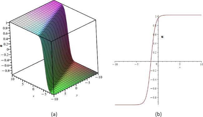
Figure 1 illustrated 3D and 2D graphical representations of the u1(x, y, t) given in equation (21), as constructed with ε = 0.1, k = −2, l = −1, m = 6, σ = 2, t = 0, y = 1. We discovered that u1 is a kink-type profile as a result of this investigating. We know that kink waves are rising or descending waves that go from one asymptotic state to another. The kink solution approaches an infinite constant [41].
Figure 1. (a) 3D-plot of u1 given in equation (21) where ε = 0.1, k = −2, l = −1, m = 6, σ = 2, t = 0, (b) 2D-plot of u1 given in equation (21) where ε = 0.1, k = −2, l = −1, m = 6, σ = 2, t = 0, y = 1.
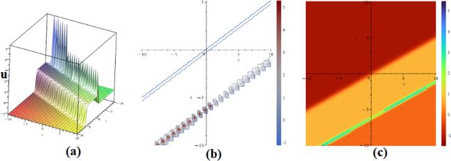
In figure 2, we presented the 3D, contour and density representations of the u2(x, y, t) interaction given in equation (36), respectively.
Figure 2. (a) 3D-plot of u4 given in equation (36), (b) Contour-plot of u4 given in equation (36), (c) Density plot of u4 given in equation (36) where s0 = 1, s1 = 3, s2 = 1, p2 = 0.3, q2 = −0.7, η1 = 1, η0 = 0.6, α = 1, σ = −0.7, x = 1.
In figure 3, the solution u5(x, y, t) given in equation (36), revealed by the interaction of a rational elliptical form solution of the equation (32) and a linear function, is presented together with s0 = 1, s1 = 3, s2 = 2, r2 = 2, q2 = −2, r1 = 1, q1 = −1, r1 = 1, r2 = 4.5, δ1 = 1, η0 = 2, α = 1, σ = 0.5, η0 = −9, and, ξ0 = 0. In figure 3 (a), 3D representation of u5(1, y, t), in (b) we demonstrate 2D plot of (u5) (1, 1, t) , (c) 3D plot of u5(x, y, t) at t = 1.
Figure 3. (a) 3D-plot of u5(1, y, t) given in equation (39), (b) 2D-plot of u5(1, 1, t) given equation (39), (c) 3D-plot of u5(x, y, 1) given in equation (39) where s0 = 1, s1 = 3, s2 = 2, r2 = 2, q2 = −2, r1 = 1, q1 = −1, r1 = 1, r2 = 4.5, δ1 = 1, η0 = 2, α = 1, σ = 0.5, η0 = −9, ξ0 = 0.

5. Conclusion

In this paper, we discussed the (2+1)-dimensional CI model, which is a well-known reaction diffusion equation. First, we applied truncated Painlevé expansion to generate the residual and Bäcklund transformations of the equation. Next, we demonstrated that the Chaffee–Infante equation is CRE solvable. To produce soliton-cnoidal wave solutions, two forms of special elliptic equation solutions are employed. Many important physical phenomena may be explored using soliton-cnoidal wave interaction solutions, including tsunami, and fermionic quantum plasma. Because the investigated equation is (2+1)-dimensional, applying the approaches is very complicated. We feel that these solutions are very distinct from those found in the literature. To the best of our knowledge, the retrieved exact solution profiles and non-local symmetry transformations are new. In addition, we have checked all the constructed exact solutions that satisfy the Chaffe-Infante equation via the Maple package program.
1
Wazwaz A M 2016 Multiple soliton solutions and multiple complex soliton solutions for two distinct Boussinesq equations Nonlinear Dyn. 85 731 737

DOI

2
Zhou T Y Tian B Shen Y Gao X T 2023 Auto-Bäcklund transformations and soliton solutions on the nonzero background for a (3+1)-dimensional Korteweg-de Vries-Calogero-Bogoyavlenskii-Schif equation in a fluid Nonlinear Dyn. 111 8647 8658

DOI

3
Wazwaz A M 2016 The simplified Hirota's method for studying three extended higher-order KdV-type equations J. Ocean Eng. Sci. 1 181 185

DOI

4
Wazwaz A M Alhejaili W AL-Ghamdi A O El-Tantawy S A 2023 Bright and dark modulated optical solitons for a (2+1)-dimensional optical Schrödinger system with third-order dispersion and nonlinearity Optik 274 170582

DOI

5
Tariq K U Wazwaz A M Javed R 2023 Construction of different wave structures, stability analysis and modulation instability of the coupled nonlinear Drinfel'd–Sokolov–Wilson model Chaos Solit. Fractals 166 112903

DOI

6
Ma W X 2022 Matrix integrable fourth-order nonlinear Schrödinger equations and their exact soliton solutions Chin. Phys. Lett. 39 100201

DOI

7
Ma W X 2023 Matrix integrable fifth-order mKdV equations and their soliton solutions Chin. Phys. B 32 020201

DOI

8
Wazwaz A M Kaur L 2019 Complex simplified Hirota's forms and Lie symmetry analysis for multiple real and complex soliton solutions of the modified KdV–Sine-Gordon equation Nonlinear Dyn. 95 2209 2215

DOI

9
Kumar S Niwas M Wazwaz A M 2020 Lie symmetry analysis, exact analytical solutions and dynamics of solitons for (2+1)-dimensional NNV equations Phys. Scr. 95 095204

DOI

10
Hirota R 2004 The Direct Method in Soliton Theory Cambridge University Press (No. 155)

DOI

11
Wazwaz A M 2007 Multiple-soliton solutions for the KP equation by Hirota's bilinear method and by the tanh-coth method Appl. Math. Comput. 190 633 640

DOI

12
Ma W X 2022 Soliton solutions by means of Hirota bilinear forms Partial Differ. Equ. Appl. Math. 5 100220

DOI

13
Wazwaz A M El-Tantawy S A 2017 Solving the (3+1)-dimensional KP–Boussinesq and BKP–Boussinesq equations by the simplified Hirota's method Nonlinear Dyn. 88 3017 3021

DOI

14
Wazwaz A M 2007 The extended tanh method for abundant solitary wave solutions of nonlinear wave equations Appl. Math. Comput. 187 1131 1142

DOI

15
Ma Y L Wazwaz A M Li B Q 2021 New extended Kadomtsev–Petviashvili equation: multiple soliton solutions, breather, lump and interaction solutions Nonlinear Dyn. 104 1581 1594

DOI

16

17
Zhao Z Han B 2018 Residual symmetry, Bäcklund transformation and CRE solvability of a (2+1 2+1)-dimensional nonlinear system Nonlinear Dyn. 94 461 474

DOI

18
Olver P J 1993 Applications of Lie Groups to Differential Equations vol 107 Springer Science & Business Media

19
Bluman G Anco S 2008 Symmetry and Integration Methods for Differential Equations vol 154 Springer Science & Business Media

20
Bluman G W Cheviakov A F Anco S C 2010 Applications of Symmetry Methods to Partial Differential Equations vol 168 Springer

21
Ibragimov N H 2009 A Practical Course in Differential Equations and Mathematical Modelling World Scientific Publishing Co Pvt Ltd

22
Chaolu T Bluman G 2014 An algorithmic method for showing existence of nontrivial non-classical symmetries of partial differential equations without solving determining equations J. Math. Anal. Appl. 411 281 296

DOI

23
Meleshko S V Grigoriev Y N Ibragimov N K Kovalev V F 2010 Symmetries of Integro-Differential Equations: With Applications in Mechanics and Plasma Physics vol 806 Springer Science & Business Media

24
Bluman G W Cheviakov A F Ivanova N M 2006 Framework for nonlocally related partial differential equation systems and nonlocal symmetries: extension, simplification, and examples J. Math. Phys. 47 113505

DOI

25
Lou S Y Hu X B 1997 Non-local symmetries via Darboux transformations J. Phys. A: Math. Nucl. Gen. 30 L95 L100

DOI

26
Hu X R Lou S Y Chen Y 2012 Explicit solutions from eigenfunction symmetry of the Korteweg–de Vries equation Phys. Rev. E 85 056607

DOI

27
Lou S Y Hu X Chen Y 2012 Nonlocal symmetries related to Bäcklund transformation and their applications J. Phys. A: Math. Theor. 45 155209

DOI

28
Chen J C Xin X P Chen Y 2014 Nonlocal symmetries of the Hirota-Satsuma coupled Korteweg–de Vries system and their applications: exact interaction solutions and integrable hierarchy J. Math. Phys. 55 053508

DOI

29
Wazwaz A M 2018 Painlevé analysis for a new integrable equation combining the modified Calogero–Bogoyavlenskii–Schiff (MCBS) equation with its negative-order form Nonlinear Dyn. 91 877 883

DOI

30
Wazwaz A M 2020 Painlevé analysis for Boiti–Leon–Manna–Pempinelli equation of higher dimensions with time-dependent coefficients: multiple soliton solutions Phys. Lett. A 384 126310

DOI

31
Liu S J Tang X Y Lou S Y 2018 Multiple Darboux–Bäcklund transformations via truncated Painlevé expansion and Lie point symmetry approach Chin. Phys. B 27 060201

DOI

32
Lou S Y 2015 Consistent Riccati expansion for integrable systems Stud. Appl. Math. 134 372 402

DOI

33
Mao Y 2018 Exact solutions to (2+1)-dimensional Chaffee–Infante equation Pramana 91 9

DOI

34
Yusuf A Sulaiman T A Abdeljabbar A Alquran M 2023 Breather waves, analytical solutions and conservation laws using Lie–Bäcklund symmetries to the (2+1)-dimensional Chaffee–Infante equation J. Ocean Eng. Sci. 8 145 151

DOI

35
Mahmood A Abbas M Akram G Sadaf M Riaz M B Abdeljawad T 2023 Solitary wave solution of (2+1)-dimensional Chaffee–Infante equation using the modified Khater method Results Phys. 48 106416

DOI

36
Riaz M B Atangana A Jhangeer A Junaid-U-Rehman M 2021 Some exact explicit solutions and conservation laws of Chaffee–Infante equation by Lie symmetry analysis Phys. Scr. 96 084008

DOI

37
Akbar M A Ali N H M Hussain J 2019 Optical soliton solutions to the (2+1)-dimensional Chaffee–Infante equation and the dimensionless form of the Zakharov equation Adv. Differ. Equ. 2019 1 18

DOI

38
Sulaiman T A Yusuf A Alquran M 2021 Dynamics of lump solutions to the variable coefficients (2+1)-dimensional Burger's and Chaffee–Infante equations J. Geom. Phys. 168 104315

DOI

39
Kumar S Almusawa H Hamid I Akbar M A Abdou M A 2021 Abundant analytical soliton solutions and evolutionary behaviors of various wave profiles to the Chaffee–Infante equation with gas diffusion in a homogeneous medium Results Phys. 30 104866

DOI

40
Ibragimov N H 1995 CRC Handbook of Lie Group Analysis of Differential Equations vol 3 CRC Press

41
Wazwaz A M 2010 Partial Differential Equations and Solitary Waves Theory Springer Science & Business Media

Outlines

/