Welcome to visit Communications in Theoretical Physics,
Mathematical Physics

Asymptotic analysis of multi-valley dark soliton solutions in defocusing coupled Hirota equations

  • Ziwei Jiang ,
  • Liming Ling , *
Expand
  • Department of Mathematics, South China University of Technology, Guangzhou 510641, China

*Author to whom any correspondence should be addressed.

Received date: 2023-05-23

  Revised date: 2023-08-08

  Accepted date: 2023-09-11

  Online published: 2023-11-10

Copyright

© 2023 Institute of Theoretical Physics CAS, Chinese Physical Society and IOP Publishing

Abstract

We construct uniform expressions of such dark soliton solutions encompassing both single-valley and double-valley dark solitons for the defocusing coupled Hirota equation with high-order nonlinear effects utilizing the uniform Darboux transformation, in addition to proposing a sufficient condition for the existence of the above dark soliton solutions. Furthermore, the asymptotic analysis we perform reveals that collisions for single-valley dark solitons typically exhibit elastic behavior; however, collisions for double-valley dark solitons are generally inelastic. In light of this, we further propose a sufficient condition for the elastic collisions of double-valley dark soliton solutions. Our results offer valuable insights into the dynamics of dark soliton solutions in the defocusing coupled Hirota equation and can contribute to the advancement of studies in nonlinear optics.

Cite this article

Ziwei Jiang , Liming Ling . Asymptotic analysis of multi-valley dark soliton solutions in defocusing coupled Hirota equations[J]. Communications in Theoretical Physics, 2023 , 75(11) : 115005 . DOI: 10.1088/1572-9494/acf84a

1. Introduction

For integrable systems, the nonlinear Schrödinger equation plays an important role in various fields such as nonlinear optics [1, 2], water waves [3, 4], plasma [5], and Bose–Einstein condensates [6]. In optical fibers, the nonlinear Schrödinger equation can describe the propagation of a picosecond optical pulse [2, 7], but for high-bit-rate transmission systems, higher-order nonlinear and dispersive effects are taken into account, which yields the higher-order nonlinear Schrödinger equation involving the Hirota equation [812]. The exact localized wave solutions of the Hirota equation, such as multi-solitons, rogue waves, and breathers, have been extensively studied [1322]. Furthermore, the explicit expressions of the asymptotic analyses of single-valley dark solitons (abbreviated as SVDS) and double-valley dark solitons (abbreviated as DVDS) have been given for the defocusing case, and a sufficient condition for elastic collisions has been obtained [21]. Notably, dark solitons with delayed nonlinear response and third-order dispersion, in contrast to those with only second-order dispersion and self-phase modulation, can admit single dark solitons with the same velocity under two different phase shifts identified as DVDSs [23]. Moreover, Hirota equations in different physical backgrounds have the characteristics of being multi-component and having variable coefficients [24]. And multi-component nonlinear systems are more widely used and possess more abundant dynamic phenomena than one-component systems [2527]. In this work, we mainly study the dark soliton solutions of the defocusing couple Hirota equation, which is completely integrable and admits the following form [2832]:
$\begin{eqnarray}{\rm{i}}{{\boldsymbol{q}}}_{t}+\displaystyle \frac{1}{2}{{\boldsymbol{q}}}_{{xx}}-{\boldsymbol{q}}{{\boldsymbol{q}}}^{\dagger }{\boldsymbol{q}}+{\rm{i}}\alpha (3{{\boldsymbol{q}}}_{x}{{\boldsymbol{q}}}^{\dagger }{\boldsymbol{q}}+3{\boldsymbol{q}}{{\boldsymbol{q}}}^{\dagger }{{\boldsymbol{q}}}_{x}-{{\boldsymbol{q}}}_{{xxx}})={\bf{0}},\end{eqnarray}$
where α is the real parameter; ${\boldsymbol{q}}={({q}_{1},{q}_{2})}^{\top }$ is a two-dimensional complex vector; the superscripts ‘⊤' and ‘†' represent the transposition and conjugate transpose of the matrix, respectively. When α = 0, equation (1) is reduced to the coupled nonlinear Schrödinger equation.
In recent years, some exact solutions of the coupled Hirota equation, such as soliton solutions [13, 33], rogue wave solutions [26, 34], breather solutions [35], and traveling wave solutions [36] have also been derived. There are transition phenomena in the evolution process between solitons, breathers, and rogue waves in the focusing case [3739]. Additionally, scholars pay attention to the dynamic behavior of the above exact solutions. For instance, elastic collisions are permitted in solutions such as SVDSs of the coupled Hirota equation [31, 40, 41]. Interestingly, in the coupled higher-order nonlinear Schrödinger equation, there exist the dark double-hump three-soliton solutions with higher order effects generated by the Hirota bilinear method, which admit elastic interactions among each other [41]. The soliton with a double-humped shape, or DVDS, has found extensive applications in power amplification processes owing to its wider pulse width and capacity to withstand higher power [42]. In fact, in the coupled Hirota equation, a single dark soliton can admit two types of intensity profiles: the dark soliton with a single valley and the dark soliton with double valleys. As far as our current state of knowledge allows us to ascertain that the question of whether there exists solely elastic interaction for DVDSs and SVDSs under the context of the coupled Hirota equation remains an open research field. The above problems in the coupled Hirota equation motivate us to further study the dynamic behaviors of its dark soliton solutions.
The paper is organized as follows: in section 2, with the aid of the uniform Darboux transformation [43], we construct uniform expressions to represent the multi-dark soliton solutions consisting of SVDSs and DVDSs for the coupled Hirota equation. Meanwhile, we propose a sufficient condition for the existence of dark soliton solutions of the coupled Hirota equation by studying the corresponding characteristic equation. In section 3, we explore the intriguing properties of these solutions through asymptotic analysis. It is revealed that the interaction among single dark soliton solutions can be divided into the following two cases: if the single dark soliton solution corresponds to an SVDS, it will inevitably result in an elastic collision. On the other hand, if the single dark soliton solution represents a DVDS, it is more likely to exhibit inelastic collision. The conclusions are given in section 4.

2. The dark soliton solutions for the coupled Hirota equation

The coupled Hirota equation (1) admits the Lax pair
$\begin{eqnarray}\begin{array}{rcl}{{\rm{\Phi }}}_{x} & = & {\boldsymbol{U}}(\lambda ;{\boldsymbol{Q}}){\rm{\Phi }},\qquad {{\rm{\Phi }}}_{t}={\boldsymbol{V}}(\lambda ;{\boldsymbol{Q}}){\rm{\Phi }},\\ {\rm{\Phi }} & = & {\rm{\Phi }}(x,t;\lambda ),\end{array}\end{eqnarray}$
where
$\begin{eqnarray*}\begin{array}{rcl}{\boldsymbol{U}} & \equiv & {\boldsymbol{U}}(\lambda ;{\boldsymbol{Q}})={\rm{i}}(\lambda {\sigma }_{3}+{\boldsymbol{Q}}),\qquad {\boldsymbol{Q}}=\left(\begin{array}{cc}0 & {{\boldsymbol{q}}}^{\dagger }\\ {\boldsymbol{q}} & {{\bf{0}}}_{2}\end{array}\right),\\ {\boldsymbol{V}} & \equiv & {\boldsymbol{V}}(\lambda ;{\boldsymbol{Q}})=(1-4\alpha \lambda )\left({\boldsymbol{U}}\lambda -\displaystyle \frac{{\rm{i}}{\sigma }_{3}}{2}({{\boldsymbol{Q}}}^{2}+{\rm{i}}{{\boldsymbol{Q}}}_{x})\right)\\ & & +{\rm{i}}\alpha ({{\boldsymbol{Q}}}_{{xx}}+2{{\boldsymbol{Q}}}^{3}-{\rm{i}}{{\boldsymbol{Q}}}_{x}{\boldsymbol{Q}}+{\rm{i}}{\boldsymbol{Q}}{{\boldsymbol{Q}}}_{x}),\end{array}\end{eqnarray*}$
σ3 = diag(1, −1, −1), $\lambda \in {\mathbb{C}}$ is a spectral parameter; q is defined in equation (1). 02 denotes the 2 × 2 null matrix. Utilizing the compatibility condition Φxt = Φtx of the Lax pair (2), we can obtain the zero curvature equation UtVx + [U, V] = 0 with [U, V] = UVVU, which results in the Hirota equation (1).
To construct dark soliton solutions, we set the plane wave solution of the coupled Hirota equation (1) as ${q}_{i}={c}_{i}{{\rm{e}}}^{{\rm{i}}{\theta }_{i}}$, where θi = aix + bit, i = 1,2, ${b}_{i}=-\alpha \left({a}_{i}^{3}+{\sum }_{j=1}^{2}3{c}_{j}^{2}({a}_{i}^{2}+{a}_{j}^{2})\right)\,-\tfrac{1}{2}{a}_{i}^{2}-{\sum }_{j\,=\,1}^{2}{c}_{j}^{2}$, ai and ci are the wave number and amplitude of background, respectively. In order to solve the Lax pair (2) with the abovementioned plane wave solution, we first convert the variable coefficient differential equation into a constant coefficient differential equation utilizing the gauge transformation $\widetilde{{\rm{\Phi }}}={\boldsymbol{G}}{\rm{\Phi }}$, $\widetilde{{\rm{\Phi }}}=\widetilde{{\rm{\Phi }}}(x,t;\lambda )$, ${\boldsymbol{G}}=\mathrm{diag}(1,{{\rm{e}}}^{-{\rm{i}}{\theta }_{1}},{{\rm{e}}}^{-{\rm{i}}{\theta }_{2}})$. It should be pointed out that the spectral parameter λ must satisfy $\lambda \in {\mathbb{R}}$ to obtain the dark soliton solutions. The Lax pair (2) is then converted into
$\begin{eqnarray}{\widetilde{{\rm{\Phi }}}}_{x}={\rm{i}}{{\boldsymbol{U}}}_{1}\widetilde{{\rm{\Phi }}},\quad {\widetilde{{\rm{\Phi }}}}_{t}={\rm{i}}(2\alpha {{\boldsymbol{U}}}_{1}^{3}+{d}_{1}{{\boldsymbol{U}}}_{1}^{2}+{d}_{2}{{\boldsymbol{U}}}_{1}+{d}_{3})\widetilde{{\rm{\Phi }}},\end{eqnarray}$
where
$\begin{eqnarray*}\begin{array}{rcl}{{\boldsymbol{U}}}_{1} & = & \left(\begin{array}{ccc}\lambda & -{c}_{1} & -{c}_{2}\\ {c}_{1} & -\lambda -{a}_{1} & 0\\ {c}_{2} & 0 & -\lambda -{a}_{2}\end{array}\right),\\ {d}_{1} & = & 3\alpha \left(\displaystyle \sum _{i=1}^{2}{a}_{i}\right)+\displaystyle \frac{1}{2},\end{array}\end{eqnarray*}$
$\begin{eqnarray*}\begin{array}{rcl}{d}_{2} & = & -6\alpha {\lambda }^{2}+\lambda +3\alpha {a}_{1}{a}_{2},\\ {d}_{3} & = & -{d}_{1}{\lambda }^{2}-3\alpha {a}_{1}{a}_{2}\lambda +\left({d}_{1}+\displaystyle \frac{1}{2}\right)\left(\displaystyle \sum _{i=1}^{2}{c}_{i}^{2}\right).\end{array}\end{eqnarray*}$
And the characteristic equation of matrix U1 is as follows:
$\begin{eqnarray}\det ({{\boldsymbol{U}}}_{1}-\mu {{\mathbb{I}}}_{3})=0,\end{eqnarray}$
where μ is the eigenvalue of equation (4) and ${{\mathbb{I}}}_{3}$ denotes the 3 × 3 identity matrix. The coefficients of the algebraic expression (4) with respect to μ are real-valued if the spectral parameter λ is real, which guarantees that expression (4) possesses either real-valued roots or a set of complex conjugate roots. To get the dark soliton solutions of equation (1), it is necessary to possess a pair of conjugate complex roots μ and μ* of equation (4). It is straightforward to obtain the vector solution of equation (3) by this pair of complex roots, and then substituting the above solution into the transformation ${\rm{\Phi }}={{\boldsymbol{G}}}^{-1}\widetilde{{\rm{\Phi }}}$ yields
$\begin{eqnarray}\begin{array}{rcl}{\rm{\Phi }} & = & \left[\begin{array}{c}{{\rm{e}}}^{{\rm{i}}X}\\ \displaystyle \frac{{c}_{1}}{\chi +{a}_{1}}{{\rm{e}}}^{{\rm{i}}(X+{\theta }_{1})}\\ \displaystyle \frac{{c}_{2}}{\chi +{a}_{2}}{{\rm{e}}}^{{\rm{i}}(X+{\theta }_{2})}\end{array}\right],\\ X & = & \mu x+(2\alpha {\mu }^{3}+{d}_{1}{\mu }^{2}+{d}_{2}\mu +{d}_{3})t,\\ \chi & = & \lambda +\mu ,\end{array}\end{eqnarray}$
which is the vector solution of equation (2).
We are going to employ the uniform Darboux transformation [43], which is widely used to generate solitonic solutions. Due to the limitations of the classical Darboux transformation, it is not feasible to directly derive the multi-dark soliton solutions of multi-component systems. Hence, we adopt the uniform Darboux transformation proposed in reference [43] to construct multi-dark soliton solutions of the coupled Hirota equation. According to equation (5), the uniform Darboux transformation can be constructed explicitly as
$\begin{eqnarray}{{\boldsymbol{T}}}^{[1]}={{\mathbb{I}}}_{3}-\displaystyle \frac{({\mu }_{1}-{\mu }_{1}^{* }){{\rm{\Phi }}}_{1}{{\rm{\Phi }}}_{1}^{\dagger }{\sigma }_{3}}{2(\lambda -{\lambda }_{1})({{\rm{e}}}^{{\rm{i}}({X}_{1}-{X}_{1}^{* })}+{{\rm{e}}}^{2{\gamma }_{1}{\mu }_{1I}})},\end{eqnarray}$
where ${{\rm{\Phi }}}_{1}={\left.{\boldsymbol{G}}{\rm{\Phi }}\right|}_{\lambda ={\lambda }_{1},\mu ={\mu }_{1}}$, ${X}_{1}=X{| }_{\lambda ={\lambda }_{1},\mu ={\mu }_{1}}$, ${\mu }_{1I}={\mathfrak{I}}({\mu }_{1})$, ${\gamma }_{1}\in {\mathbb{R}}$ is an arbitrary constant. Furthermore, the SVDS corresponding to the spectral parameter λ1 for the coupled Hirota equation (1) can be expressed as
$\begin{eqnarray}\begin{array}{rcl}{{\boldsymbol{q}}}^{[1]}(x,t;{{\boldsymbol{c}}}_{1}^{(s)}) & = & {\left[{q}_{1}^{[1]}(x,t;{{\boldsymbol{c}}}_{1}^{(s)}),{q}_{2}^{[1]}(x,t;{{\boldsymbol{c}}}_{1}^{(s)})\right]}^{\top },\\ {q}_{i}^{[1]}(x,t;{{\boldsymbol{c}}}_{1}^{(s)}) & = & {c}_{i}\left(1-\displaystyle \frac{{B}_{i}}{2}+\displaystyle \frac{{B}_{i}}{2}\tanh ({Y}_{1})\right){{\rm{e}}}^{{\rm{i}}{\theta }_{i}},\end{array}\end{eqnarray}$
where ${{\boldsymbol{c}}}_{1}^{(s)}=\left({\lambda }_{1},{\gamma }_{1},{\mu }_{1}\right)$, ${\mu }_{1R}={\mathfrak{R}}({\mu }_{1})$, ${B}_{i}=\tfrac{{\mu }_{1}-{\mu }_{1}^{* }}{{\chi }_{1}+{a}_{i}}$, i = 1, 2, ${v}_{1}=-(2\alpha (3{\left({\mu }_{1R}\right)}^{2}-{\left({\mu }_{1I}\right)}^{2})+2{d}_{1}{\mu }_{1R}+{d}_{2})$, Y1 = μ1I(xv1t + γ1) and v1 represents the velocity of SVDS (7). According to solution (7), we could obtain the following straightforward features about SVDSs: the evolution direction of dark soliton solution (7) is along the trajectory xv1t + γ1 = 0; the valley depths of ${\left|{q}_{i}^{[1]}\right|}^{2}$, i = 1, 2 are $\tfrac{{c}_{i}^{2}{\left({\mu }_{1I}\right)}^{2}}{{\left({\lambda }_{1}+{a}_{i}+{\mu }_{1R}\right)}^{2}+{\left({\mu }_{1I}\right)}^{2}}$, respectively.
We select a set of parameters based on equation (7), allowing us to successfully present the density profile of the SVDS, as shown in figure 1. In particular, substituting the parameters a1 = 1, a2 = −0.4, c1 = 1, c2 = 1, and λ1 = 1 into the characteristic equation (4) to yield the complex root μ1 ≈ −0.2513 + 1.2203i and then substituting all parameters into the above results, we can obtain that: the velocity v1 of the dark soliton solution is approximately equal to 4.6289; the valley depths of ${\left|{q}_{1}^{[1]}\right|}^{2}$ and ${\left|{q}_{2}^{[1]}\right|}^{2}$ are approximately equal to 0.9601 and 0.5291, respectively; the evolution direction of dark soliton solution is along the trajectory xv1t − 0.5 = 0, v1 ≈ 4.6289.
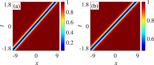
Figure 1. The density profiles of intensity square of the dark soliton solution with the parameters ${{\boldsymbol{c}}}_{1}^{(s)}\approx \left(-0.5,1,-0.2513+1.2203{\rm{i}}\right)$, a1 = 1, a2 = −0.4, c1 = 1, c2 = 1, and α = 0.65, which corresponds to an SVDS. (a) The density profile of $| {q}_{1}^{[1]}{| }^{2}$. (b) The density profile of $| {q}_{2}^{[1]}{| }^{2}$.
Similarly, we are able to construct the expressions of the multi-dark soliton solutions corresponding to the spectral parameters λi, i = 1, 2, ⋯ , n for the coupled Hirota equation (1). Suppose that Lax pair (2) has n different solutions ${{\rm{\Phi }}}_{i}={\left.{\boldsymbol{G}}{\rm{\Phi }}\right|}_{\lambda ={\lambda }_{i},\mu ={\mu }_{i}}$, and ${{\rm{\Phi }}}_{j}^{\dagger }{\sigma }_{3}{{\rm{\Phi }}}_{j}=0$, if ${\lambda }_{j}\in {\mathbb{R}}$ , then the n-fold uniform Darboux transformation can be expressed as
$\begin{eqnarray}{{\boldsymbol{T}}}^{[n]}={{\mathbb{I}}}_{3}-{{\rm{\Theta }}}_{n}{{\boldsymbol{R}}}_{n}^{-1}{\left(\lambda {{\mathbb{I}}}_{n}-{{\boldsymbol{D}}}_{n}\right)}^{-1}{{\rm{\Theta }}}_{n}^{\dagger }{\sigma }_{3},\end{eqnarray}$
where
$\begin{eqnarray*}\begin{array}{rcl}{{\rm{\Theta }}}_{n} & = & \left[{{\rm{\Phi }}}_{1},{{\rm{\Phi }}}_{2},\cdots ,{{\rm{\Phi }}}_{n}\right],{{\boldsymbol{D}}}_{n}=\mathrm{diag}({\lambda }_{1},{\lambda }_{2},\ldots ,{\lambda }_{n}),{\nu }_{j}=\displaystyle \frac{1}{{\rm{i}}{\mu }_{{jI}}}{{\rm{e}}}^{2{\gamma }_{j}{\mu }_{{jI}}},j\,=\,1,2,\cdots ,n,\\ {{\boldsymbol{R}}}_{n} & = & \left[\begin{array}{cccc}\mathop{\mathrm{lim}}\limits_{\lambda \to {\lambda }_{1}}\displaystyle \frac{{{\rm{\Phi }}}_{1}^{\dagger }{\rm{\Lambda }}{{\rm{\Phi }}}_{1}(\lambda )}{\lambda -{\lambda }_{1}}+{\nu }_{1} & \displaystyle \frac{{{\rm{\Phi }}}_{1}^{\dagger }{\sigma }_{3}{{\rm{\Phi }}}_{2}}{{\lambda }_{2}-{\lambda }_{1}} & \cdots & \displaystyle \frac{{{\rm{\Phi }}}_{1}^{\dagger }{\sigma }_{3}{{\rm{\Phi }}}_{n}}{{\lambda }_{n}-{\lambda }_{1}}\\ \displaystyle \frac{{{\rm{\Phi }}}_{2}^{\dagger }{\sigma }_{3}{{\rm{\Phi }}}_{1}}{{\lambda }_{1}-{\lambda }_{2}} & \mathop{\mathrm{lim}}\limits_{\lambda \to {\lambda }_{2}}\displaystyle \frac{{{\rm{\Phi }}}_{2}^{\dagger }{\sigma }_{3}{{\rm{\Phi }}}_{2}(\lambda )}{\lambda -{\lambda }_{2}}+{\nu }_{2} & \cdots & \displaystyle \frac{{{\rm{\Phi }}}_{2}^{\dagger }{\sigma }_{3}{{\rm{\Phi }}}_{n}}{{\lambda }_{n}-{\lambda }_{2}}\\ \vdots & \vdots & \ddots & \vdots \\ \displaystyle \frac{{{\rm{\Phi }}}_{n}^{\dagger }{\sigma }_{3}{{\rm{\Phi }}}_{1}}{{\lambda }_{1}-{\lambda }_{n}} & \displaystyle \frac{{{\rm{\Phi }}}_{n}^{\dagger }{\sigma }_{3}{{\rm{\Phi }}}_{2}}{{\lambda }_{2}-{\lambda }_{n}} & \cdots & \mathop{\mathrm{lim}}\limits_{\lambda \to {\lambda }_{n}}\displaystyle \frac{{{\rm{\Phi }}}_{n}^{\dagger }{\sigma }_{3}{{\rm{\Phi }}}_{n}(\lambda )}{\lambda -{\lambda }_{n}}+{\nu }_{n}\end{array}\right].\end{array}\end{eqnarray*}$

The expressions for the multi-dark soliton solutions can be derived by the n-fold uniform Darboux transformation (8):

$\begin{eqnarray}\begin{array}{rcl}{{\boldsymbol{q}}}^{[n]}(x,t;{\boldsymbol{c}}) & = & {\left[{q}_{1}^{[n]}(x,t;{\boldsymbol{c}}),{q}_{2}^{[n]}(x,t;{\boldsymbol{c}})\right]}^{\top },\\ {q}_{i}^{[n]}(x,t;{\boldsymbol{c}}) & = & {c}_{i}\displaystyle \frac{\det ({{\boldsymbol{M}}}_{i})}{\det ({\boldsymbol{N}})}{{\rm{e}}}^{{\rm{i}}{\theta }_{i}},\end{array}\end{eqnarray}$
where
$\begin{eqnarray}\begin{array}{rcl}{{\boldsymbol{M}}}_{i} & = & {\left(\displaystyle \frac{2\left({{\rm{e}}}^{{\rm{i}}({X}_{l}-{X}_{k}^{* })}+{\delta }_{k,l}\right)}{{\chi }_{l}-{\chi }_{k}^{* }}-2{\beta }_{l,i}{{\rm{e}}}^{{\rm{i}}({X}_{l}-{X}_{k}^{* })}\right)}_{1\leqslant k,l\leqslant n},\\ {\beta }_{l,i} & = & \displaystyle \frac{1}{{a}_{i}+{\chi }_{l}},\\ {\boldsymbol{N}} & = & {\left(\displaystyle \frac{2\left({{\rm{e}}}^{{\rm{i}}({X}_{l}-{X}_{k}^{* })}+{\delta }_{k,l}\right)}{{\chi }_{l}-{\chi }_{k}^{* }}\right)}_{1\leqslant k,l\leqslant n},\\ {\delta }_{k,l} & = & \left\{\begin{array}{ll}0, & k\ne l\\ {{\rm{e}}}^{2{\gamma }_{k}{\mu }_{{kI}}}, & k=l\end{array}\right.,\quad {\chi }_{l}={\lambda }_{l}+{\mu }_{l},\end{array}\end{eqnarray}$
Xl is defined in equation (5), ${\boldsymbol{c}}=({\lambda }_{1},{\lambda }_{2},\cdots ,{\lambda }_{n},{\gamma }_{1},{\gamma }_{2},\cdots ,{\gamma }_{n},{\mu }_{1},{\mu }_{2},\cdots ,{\mu }_{n})$. In fact, a multi-dark soliton ${{\boldsymbol{q}}}^{[n]}(x,t;{\boldsymbol{c}})$ can be seen as consisting of ns SVDSs and nd DVDSs. The SVDS corresponding to the spectral parameter ${\lambda }_{l}$ is defined as ${{\boldsymbol{q}}}^{[1]}(x,t;{{\boldsymbol{c}}}_{l}^{(s)})=[{q}_{1}^{[1]}(x,t;{{\boldsymbol{c}}}_{l}^{(s)}),{q}_{2}^{[1]}{(x,t;{{\boldsymbol{c}}}_{l}^{(s)})]}^{\top }$, and the DVDS with ${v}_{l-1}={v}_{l}$ corresponding to the spectral parameters ${\lambda }_{l-1}$ and ${\lambda }_{l}$ is denoted as ${{\boldsymbol{q}}}^{[2]}(x,t;{{\boldsymbol{c}}}_{l}^{(d)})={\left[{q}_{1}^{[2]}(x,t;{{\boldsymbol{c}}}_{l}^{(d)}),{q}_{2}^{[2]}(x,t;{{\boldsymbol{c}}}_{l}^{(d)})\right]}^{\top }$, where ${v}_{l}=-(2\alpha (3{\left({\mu }_{{lR}}\right)}^{2}-{\left({\mu }_{{lI}}\right)}^{2})+2{d}_{1}{\mu }_{{lR}}+{d}_{2})$, ${{\boldsymbol{c}}}_{l}^{(d)}=\left({\lambda }_{l-1},{\lambda }_{l},{\gamma }_{l-1},{\gamma }_{l},{\mu }_{l-1},{\mu }_{l}\right)$, $l=2,3,\cdots n$.

We select two sets of parameters to construct two types of multi-dark soliton solutions respectively. The multi-dark soliton solution in figure 2 exhibits the dynamics of three SVDSs, whereas the multi-dark soliton solution in figure 3 displays the dynamics of a DVDS and an SVDS. Notably, in contrast to the scalar Hirota equation, the two valleys of the DVDS can remain relatively far away from each other.
Figure 2. The density profiles of intensity square of the dark soliton solution with the parameters ns = 3, nd = 0, a1 = 0.5, a2 = −0.4, c1 = 1, c2 = 1, α = 0.625, and c ≈ (1, 0.5, −1, 1, 1.2, 10, 0.0686 + 0.9824i, 0.0302 + 1.2606i, − 0.1154 + 1.0236i), which corresponds to a general multi-dark soliton solution. (a) The density profile of $| {q}_{1}^{[3]}{| }^{2}$. (b) The density profile of $| {q}_{2}^{[3]}{| }^{2}$.
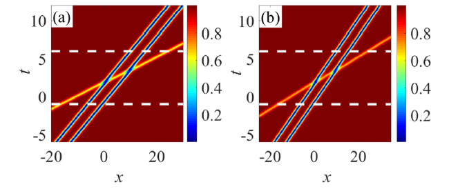
Figure 3. The density profiles of the intensity square of the dark soliton solution with the parameters ns = 1, nd = 1, a1 = − 0.2, a2 = − 0.4, c1 = 1, c2 = 1, α = 0.625, and ${\boldsymbol{c}}\approx \left(0.15,0.1,-1,1,1.2,10,0.15-1.4107{\rm{i}},0.1498+1.498{\rm{i}},0.1443+0.8251{\rm{i}}\right)$, which corresponds to a multi-dark soliton consisting of a symmetric DVDS and an SVDS. (a) The density profile of $| {q}_{1}^{[3]}{| }^{2}$. (b) The density profile of $| {q}_{2}^{[3]}{| }^{2}$.
Whilst it is true that not all parameters selected can yield a dark soliton solution for the coupled Hirota equation, we shall endeavor to identify the underlying conditions that satisfy the existence of such solutions. Especially, we restrict our attention to the case of a1 > a2 and c1 = c2 in the subsequent proposition.

If the following conditions $(1)$ or $(2)$ hold:

1.

(1)$\lambda \in \left(\tfrac{{{\rm{\Delta }}}_{3}-\sqrt{{{\rm{\Delta }}}_{1}+\sqrt{{{\rm{\Delta }}}_{2}}}}{4\left({a}_{1}-{a}_{2}\right)},\tfrac{{{\rm{\Delta }}}_{3}-\sqrt{{{\rm{\Delta }}}_{1}-\sqrt{{{\rm{\Delta }}}_{2}}}}{4\left({a}_{1}-{a}_{2}\right)}\right)$∪$\left(\tfrac{{{\rm{\Delta }}}_{3}+\sqrt{{{\rm{\Delta }}}_{1}-\sqrt{{{\rm{\Delta }}}_{2}}}}{4\left({a}_{1}-{a}_{2}\right)},\tfrac{{{\rm{\Delta }}}_{3}+\sqrt{{{\rm{\Delta }}}_{1}+\sqrt{{{\rm{\Delta }}}_{2}}}}{4\left({a}_{1}-{a}_{2}\right)}\right)$ with ${\left({a}_{1}-{a}_{2}\right)}^{2}\geqslant 8{c}_{1}^{2}$,

2.

(2)$\lambda \in \left(\tfrac{{{\rm{\Delta }}}_{3}-\sqrt{{{\rm{\Delta }}}_{1}-\sqrt{{{\rm{\Delta }}}_{2}}}}{4\left({a}_{1}-{a}_{2}\right)},\tfrac{{{\rm{\Delta }}}_{3}+\sqrt{{{\rm{\Delta }}}_{1}-\sqrt{{{\rm{\Delta }}}_{2}}}}{4\left({a}_{1}-{a}_{2}\right)}\right)$ with ${\left({a}_{1}-{a}_{2}\right)}^{2}\lt 8{c}_{1}^{2}$,

where ${{\rm{\Delta }}}_{1}={\left({a}_{1}-{a}_{2}\right)}^{4}\,+\,20{\left({a}_{1}-{a}_{2}\right)}^{2}{c}_{1}^{2}-8{c}_{1}^{4}$, ${{\rm{\Delta }}}_{2}\,=64{c}_{1}^{2}{\left({\left({a}_{1}-{a}_{2}\right)}^{2}+{c}_{1}^{2}\right)}^{3}$, ${{\rm{\Delta }}}_{3}={a}_{2}^{2}-{a}_{1}^{2}$, then the defocusing coupled Hirota equation admits the dark soliton solutions.

In order to construct dark soliton solutions by uniform Darboux transformation, equation (4) ought to admit a pair of conjugate complex roots. Considering that μ serves as an eigenvalue of matrix ${{\boldsymbol{U}}}_{1}$, we identify the discriminant of this equation with respect to μ to obtain

$\begin{eqnarray*}{\rm{\Delta }}=-\displaystyle \frac{3\left({\left({\left({a}_{1}-{a}_{2}\right)}^{2}{\left(4\lambda +({a}_{1}+{a}_{2})\right)}^{2}-{{\rm{\Delta }}}_{1}\right)}^{2}-{{\rm{\Delta }}}_{2}\right)}{16{\left({a}_{1}-{a}_{2}\right)}^{2}}.\end{eqnarray*}$
According to the Cardan formula, when ${\rm{\Delta }}\leqslant 0$, (4) has three real roots; when ${\rm{\Delta }}\gt 0$, (4) has a real root and a pair of conjugate complex roots, which ensures the existence of the dark soliton solutions of equation (1). As previously discussed, we only need to consider ${\rm{\Delta }}\gt 0$. In this case, λ is located in $\left(\tfrac{{{\rm{\Delta }}}_{3}-\sqrt{{{\rm{\Delta }}}_{1}+\sqrt{{{\rm{\Delta }}}_{2}}}}{4\left({a}_{1}-{a}_{2}\right)},\tfrac{{{\rm{\Delta }}}_{3}-\sqrt{{{\rm{\Delta }}}_{1}-\sqrt{{{\rm{\Delta }}}_{2}}}}{4\left({a}_{1}-{a}_{2}\right)}\right)$ ∪$\left(\tfrac{{{\rm{\Delta }}}_{3}+\sqrt{{{\rm{\Delta }}}_{1}-\sqrt{{{\rm{\Delta }}}_{2}}}}{4\left({a}_{1}-{a}_{2}\right)},\tfrac{{{\rm{\Delta }}}_{3}+\sqrt{{{\rm{\Delta }}}_{1}+\sqrt{{{\rm{\Delta }}}_{2}}}}{4\left({a}_{1}-{a}_{2}\right)}\right)$, where ${\left({a}_{1}-{a}_{2}\right)}^{2}\geqslant 8{c}_{1}^{2}$ guarantees ${{\rm{\Delta }}}_{1}\geqslant {{\rm{\Delta }}}_{2}^{2}$ established, whereas without this condition, λ is located in $\left(\tfrac{{{\rm{\Delta }}}_{3}-\sqrt{{{\rm{\Delta }}}_{1}-\sqrt{{{\rm{\Delta }}}_{2}}}}{4\left({a}_{1}-{a}_{2}\right)},\tfrac{{{\rm{\Delta }}}_{3}+\sqrt{{{\rm{\Delta }}}_{1}-\sqrt{{{\rm{\Delta }}}_{2}}}}{4\left({a}_{1}-{a}_{2}\right)}\right)$.

We can perform a similar analysis in the absence of the restrictions of a1 > a2 and c1 = c2, but we are unable to provide an explicit expression of the existence condition of the solution (9). In order to vividly demonstrate the relationship between parameters and the existence of dark soliton solutions, we plot figure 4. It is worth noting that the dark soliton solutions exist solely in the X-type region, with no such solutions being present in other regions. Moreover, the color bar in figure 4 indicates that the velocity of the dark soliton solution varies monotonically within some intervals. This figure agrees with the conditions of the existence of dark soliton solutions for the coupled Hirota equation (1).
Figure 4. The existence and velocity variation of the dark soliton solutions. The parameters are a2 = −0.4, c1 = c2 = 1, α = 0.625. The white square corresponds to the dark soliton solution in figure 1, the green triangle to the dark soliton solution in figure 2, and the pink pentagram to the special dark soliton solution in figure 3. The parameter selections of the solutions depicted in this figure are consistent with the requirement for the existence of solutions as stipulated in lemma 1.

3. The asymptotic analysis of the dark soliton solutions

In this section, we primarily employ asymptotic analysis to explore the evolution of the exact solutions for the coupled Hirota equation, which are composed of SVDSs and DVDSs.

For the multi-dark soliton solutions ${q}_{i}^{[n]}(x,t;{\boldsymbol{c}})$, $n={n}_{s}+2{n}_{d}$, i = 1, 2, composed of ns SVDSs and nd DVDSs, we define trajectories for SVDSs and DVDSs, respectively.

1.

(1)In the case of SVDSs, suppose ${v}_{1}^{(s)}\gt {v}_{2}^{(s)}\gt \cdots \gt {v}_{{n}_{s}}^{(s)}$, then we define the trajectories lj as $x-{v}_{j}^{(s)}t\,\equiv \mathrm{const}$, $j=1,2,\cdots ,{n}_{s}$.

2.

(2)In the case of DVDSs, suppose ${v}_{1}^{(d)}\gt {v}_{2}^{(d)}\gt \cdots \gt {v}_{{n}_{d}}^{(d)}$, then we define the trajectories Lj as $x-{v}_{j}^{(d)}t\,\equiv \mathrm{const}$, $j=1,2,\cdots ,{n}_{d}$.

We arrange all the velocities ${v}_{j}^{(s)}$, j = 1, 2, ⋯ , ns and ${v}_{j}^{(d)}$, j = 1, 2, ⋯ , nd in descending order as ${v}_{1}^{{\prime} }\gt {v}_{2}^{{\prime} }\gt \cdots \gt {v}_{{n}_{s}+{n}_{d}}^{{\prime} }$ resulting in a total of $\left(\displaystyle \genfrac{}{}{0em}{}{{n}_{s}+{n}_{d}}{{n}_{d}}\right)$ possible arrangements, and then we obtain the trajectories hj, j = 1, 2, ⋯ , ns + nd corresponding to the velocities ${v}_{j}^{{\prime} }$, j = 1, 2, ⋯ ,ns + nd, where hjSlSL, ${{\boldsymbol{S}}}_{l}={\{{l}_{j}\}}_{j=1}^{{n}_{s}}$ and ${{\boldsymbol{S}}}_{L}={\{{L}_{j}\}}_{j=1}^{{n}_{d}}$. Note that ${q}_{i}^{[n]}(x,t;{\boldsymbol{c}})$ corresponds to spectral parameters λj, j = 1, 2, ⋯ n, where each DVDS corresponds to two distinct spectral parameters. We can also define the trajectories according to the number of the spectral parameters λj. Suppose that the velocities vj, j = 1, 2, ⋯ , n corresponding to λj satisfy v1v2 ≥ ⋯ ≥ vn, where vjV(s)V(d), ${{\boldsymbol{V}}}^{(s)}=\{{v}_{j}^{(s)}\}{}_{j\,=\,1}^{{n}_{s}}$, ${{\boldsymbol{V}}}^{(d)}=\{{v}_{j}^{(d)}\}{}_{j\,=\,1}^{{n}_{d}}$, we define the trajectories gj as $x-{v}_{j}t\equiv \mathrm{const}$, j = 1, 2, ⋯ , ns + 2nd, where gjSlSL. In order to distinguish whether the trajectory gj at the jth location corresponds to an SVDS or DVDS, we modify the subscripts of lj, j = 1, 2, ⋯ , ns and Lj, j = 1, 2, ⋯ , nd to their corresponding subscript of gj, j = 1, 2, ⋯ , n. Note that if gj−1SL and gjSL, then gj−1 = gj, and we only take the subscript of L as j. For the sake of clarity, we provide an illustrative example. Suppose that the velocities vj, j = 1, 2, 3 corresponding to λj, j = 1, 2, 3 satisfy v1 > v2v3. We define the trajectories gj, j = 1, 2, 3 where g1, g2 and g3 are l1, L1 and L1, respectively, and then we modify l1 to l1 and L1 to L3.

Set the matrices

$\begin{eqnarray}\begin{array}{rcl}{\boldsymbol{A}} & = & {\left(\displaystyle \frac{2}{{\chi }_{l}-{\chi }_{k}^{* }}\right)}_{1\leqslant k,l\leqslant n},\quad {\boldsymbol{B}}={\left(\displaystyle \frac{2{\delta }_{k,l}}{{\chi }_{l}-{\chi }_{k}^{* }}\right)}_{1\leqslant k,l\leqslant n},\\ {\boldsymbol{C}} & = & {\left(\displaystyle \frac{2}{{\chi }_{l}-{\chi }_{k}^{* }}-2{\beta }_{l,k}\right)}_{1\leqslant k,l\leqslant n},\end{array}\end{eqnarray}$
where ${\chi }_{l}$, ${\beta }_{l,k}$ and ${\delta }_{k,l}$ are defined in equation (10). The determinants of matrices ${\boldsymbol{A}}$, ${\boldsymbol{B}}$, and ${\boldsymbol{C}}$ are $\det ({\boldsymbol{A}})\,={2}^{n}\tfrac{{\prod }_{1\leqslant k\lt l\leqslant n}(-{\chi }_{l}^{* }+{\chi }_{k}^{* })({\chi }_{l}-{\chi }_{k})}{{\prod }_{k\,=\,1}^{n}{\prod }_{l\,=\,1}^{n}({\chi }_{l}-{\chi }_{k}^{* })}$, $\det ({\boldsymbol{B}})={2}^{n}\tfrac{{{\rm{e}}}^{2{\sum }_{k\,=\,1}^{n}{\gamma }_{k}{\mu }_{{kI}}}}{{\prod }_{k\,=\,1}^{n}({\chi }_{k}-{\chi }_{k}^{* })}$, $\det ({\boldsymbol{C}})\,={\prod }_{k\,=\,1}^{n}\tfrac{{a}_{i}+{\chi }_{k}^{* }}{{a}_{i}+{\chi }_{k}}\det ({\boldsymbol{A}})$.

Matrix ${\boldsymbol{A}}$ is a Cauchy matrix and matrix ${\boldsymbol{B}}$ is a diagonal matrix, thus we can directly identify the determinants of them. Additionally, matrix ${\boldsymbol{C}}$ can be rewritten as ${\boldsymbol{C}}={\left(\tfrac{{a}_{i}+{\chi }_{k}^{* }}{{a}_{i}+{\chi }_{l}}\tfrac{2}{{\chi }_{l}-{\chi }_{k}^{* }}\right)}_{1\leqslant k,l\leqslant n}$, enabling us to obtain the determinant of matrix ${\boldsymbol{C}}$.

For convenience, we introduce the following notations:
$\begin{eqnarray}\begin{array}{rcl}{\xi }_{j}^{+} & = & \left\{\begin{array}{ll}0, & {v}_{j}={v}_{j+1}\\ \displaystyle \prod _{k=j+1}^{n}\displaystyle \frac{{a}_{i}+{\chi }_{k}^{* }}{{a}_{i}+{\chi }_{k}}, & {\rm{otherwise}}\end{array}\right.,\\ {\xi }_{j}^{-} & = & \left\{\begin{array}{ll}0, & {v}_{j}={v}_{j+1}\\ \displaystyle \prod _{k=1}^{j-2}\displaystyle \frac{{a}_{i}+{\chi }_{k}^{* }}{{a}_{i}+{\chi }_{k}}, & {v}_{j-1}={v}_{j}\\ \displaystyle \prod _{k=1}^{j-1}\displaystyle \frac{{a}_{i}+{\chi }_{k}^{* }}{{a}_{i}+{\chi }_{k}}, & {\rm{otherwise}}\end{array}\right.,\\ {\left({\zeta }_{j}^{[k]}\right)}^{-} & = & \left\{\begin{array}{ll}\displaystyle \prod _{l=1}^{j-2}{\left|{\chi }_{l}-{\chi }_{k}\right|}^{2}, & {v}_{j-1}={v}_{j}\\ \displaystyle \prod _{l=1}^{j-1}{\left|{\chi }_{l}-{\chi }_{k}\right|}^{2}, & {\rm{otherwise}}\end{array}\right.,\\ {\left({\zeta }_{j}^{[k]}\right)}^{+} & = & \displaystyle \prod _{l=j+1}^{n}{\left|{\chi }_{l}-{\chi }_{k}\right|}^{2},\\ {\left({\tilde{\zeta }}_{j}^{[k]}\right)}^{+} & = & \displaystyle \prod _{l=j+1}^{n}{\left|{\chi }_{l}^{* }-{\chi }_{k}\right|}^{2},\\ {\left({\tilde{\zeta }}_{j}^{[k]}\right)}^{-} & = & \left\{\begin{array}{ll}\displaystyle \prod _{l=1}^{j-2}{\left|{\chi }_{l}^{* }-{\chi }_{k}\right|}^{2}, & {v}_{j-1}={v}_{j}\\ \displaystyle \prod _{l=1}^{j-1}{\left|{\chi }_{l}^{* }-{\chi }_{k}\right|}^{2}, & {\rm{otherwise}}\end{array}\right.,\end{array}\end{eqnarray}$
where χj = λj + μj, the velocity vj is an expression related to λj. Indeed, we express the velocity vj in terms of the parameter μj as specified in equation (7). Notably, since the parameter μj and λj are conjoined via the characteristic equation (4), the velocity vj is inherently linked to λj as well. With the aforementioned notational framework and results established, we are now poised to undertake an asymptotic analysis [44] of the dynamic behavior exhibited by both SVDSs and DVDSs.

As $t\to \pm \infty $ , the multi-dark soliton solutions ${q}_{i}^{[n]}(x,t;{\boldsymbol{c}})$ in equation (9) corresponding to spectral parameters ${\lambda }_{j}$, $j=1,2,\cdots ,n$, are approximately expressed as a sum of single dark soliton solutions as follows:

$\begin{eqnarray}{q}_{i}^{[n]}(x,t;{\boldsymbol{c}})=\displaystyle \sum _{j=1}^{n}{\xi }_{j}^{\pm }({q}_{i}^{\pm }(x,t;{{\boldsymbol{c}}}_{j}^{(p)})-{c}_{i}{{\rm{e}}}^{{\rm{i}}{\theta }_{i}})+{ \mathcal O }({{\rm{e}}}^{-\epsilon | t| }),\end{eqnarray}$
where i = 1, 2, p = s, d, $\epsilon ={\min }_{1\leqslant k\ne j\leqslant n}\left(| {v}_{k}-{v}_{j}| \right)$.
i

(i)As ${v}_{j-1}\ne {v}_{j}$ and ${v}_{j}\ne {v}_{j+1}$, ${q}_{i}^{\pm }(x,t;{{\boldsymbol{c}}}_{j}^{(s)})$ is the SVDS ${q}_{i}^{[1]}(x,t;{{\boldsymbol{c}}}_{j}^{(s)})$ with a shift ${x}_{0j}^{\pm }$, and its expression is

$\begin{eqnarray}{q}_{i}^{\pm }(x,t;{{\boldsymbol{c}}}_{j}^{(s)})={c}_{i}\left(1-{B}_{j}+{B}_{j}\tanh ({Y}_{j}^{\pm })\right){{\rm{e}}}^{{\rm{i}}{\theta }_{i}},\end{eqnarray}$
where ${Y}_{j}^{\pm }=x-{v}_{j}t+{\gamma }_{j}+{x}_{0j}^{\pm }$, ${x}_{0j}^{\pm }=-\tfrac{1}{2}\mathrm{ln}(\tfrac{{\left({\zeta }_{j}^{[j]}\right)}^{\pm }}{{\left({\tilde{\zeta }}_{j}^{[j]}\right)}^{\pm }})$, ${\gamma }_{j}$ and Bj are defined in equations (6) and (7), respectively.

ii

(ii)As ${v}_{j-1}={v}_{j}$, ${q}_{i}^{\pm }(x,t;{{\boldsymbol{c}}}_{j}^{(d)})$ represents a DVDS and its expression is

$\begin{eqnarray}{q}_{i}^{\pm }(x,t;{{\boldsymbol{c}}}_{j}^{(d)})={c}_{i}\displaystyle \frac{\det ({\hat{{\boldsymbol{M}}}}_{i}^{\pm })}{\det ({\hat{{\boldsymbol{N}}}}^{\pm })}{{\rm{e}}}^{{\rm{i}}{\theta }_{i}},\end{eqnarray}$
where
$\begin{eqnarray}\begin{array}{rcl}{\hat{{\boldsymbol{M}}}}_{i}^{\pm } & = & {\left(\displaystyle \frac{[{{\rm{e}}}^{{\rm{i}}({\hat{X}}_{l}^{\pm }-{\left({\widetilde{X}}_{k}^{\pm }\right)}^{* })}+{\delta }_{k,l}]}{{\chi }_{l}-{\chi }_{k}^{* }}-{\beta }_{l,i}{{\rm{e}}}^{{\rm{i}}({\hat{X}}_{l}^{\pm }-{\left({\widetilde{X}}_{k}^{\pm }\right)}^{* })}\right)}_{j-1\leqslant k,l\leqslant j},\\ {\hat{{\boldsymbol{N}}}}^{\pm } & = & {\left(\displaystyle \frac{[{{\rm{e}}}^{{\rm{i}}({\hat{X}}_{l}^{\pm }-{\left({\widetilde{X}}_{k}^{\pm }\right)}^{* })}+{\delta }_{k,l}]}{{\chi }_{l}-{\chi }_{k}^{* }}\right)}_{j-1\leqslant k,l\leqslant j},\end{array}\end{eqnarray}$
${\hat{X}}_{l}^{\pm }={X}_{l}+\mathrm{ln}({\left({\zeta }_{j}^{[l]}\right)}^{\pm })$, ${\widetilde{X}}_{l}^{\pm }={X}_{l}+\mathrm{ln}({\left({\tilde{\zeta }}_{j}^{[l]}\right)}^{\pm })$, ${\hat{{\boldsymbol{M}}}}_{i}^{\pm }$ and ${\hat{{\boldsymbol{N}}}}^{\pm }$ are both 2 × 2 matrices; ${\beta }_{l,i}$ and ${\delta }_{k,l}$ are defined in equation (10).

The proof of theorem 2 mainly comprises two paragraphs: one is the asymptotic expressions for multi-dark soliton solutions ${q}_{i}^{[n]}(x,t;{\boldsymbol{c}})$ along the trajectory lj, and the other is along the trajectory Lj. To begin, we perform the asymptotic analysis of the multi-dark soliton solutions along the trajectory lj. The expressions of the multi-dark soliton solutions (9) can be written as

$\begin{eqnarray}{q}_{i}^{[n]}(x,t;{\boldsymbol{c}})={c}_{i}\displaystyle \frac{\det ({{\boldsymbol{E}}}^{\dagger }{\boldsymbol{C}}{\boldsymbol{E}}+{\boldsymbol{B}})}{\det ({{\boldsymbol{E}}}^{\dagger }{\boldsymbol{A}}{\boldsymbol{E}}+{\boldsymbol{B}})}{{\rm{e}}}^{{\rm{i}}{\theta }_{i}},\end{eqnarray}$
where matrices ${\boldsymbol{A}}$, ${\boldsymbol{B}}$, ${\boldsymbol{C}}$ are defined in lemma 1 and
$\begin{eqnarray}{\boldsymbol{E}}=\mathrm{diag}\left({{\rm{e}}}^{{\rm{i}}{X}_{1}},{{\rm{e}}}^{{\rm{i}}{X}_{2}},\cdots ,{{\rm{e}}}^{{\rm{i}}{X}_{n}}\right).\end{eqnarray}$
Moreover, the multi-dark soliton solutions can be expressed as
$\begin{eqnarray}\begin{array}{l}{q}_{i}^{[n]}(x,t;{\boldsymbol{c}})\\ \quad ={c}_{i}\displaystyle \frac{\det ({\left({{\boldsymbol{F}}}_{j}^{\pm }\right)}^{\dagger }{{\boldsymbol{E}}}^{\dagger }{\boldsymbol{C}}{\boldsymbol{E}}{{\boldsymbol{F}}}_{j}^{\pm }+{\left({{\boldsymbol{F}}}_{j}^{\pm }\right)}^{\dagger }{\boldsymbol{B}}{{\boldsymbol{F}}}_{j}^{\pm })}{\det ({\left({{\boldsymbol{F}}}_{j}^{\pm }\right)}^{\dagger }{{\boldsymbol{E}}}^{\dagger }{\boldsymbol{A}}{\boldsymbol{E}}{{\boldsymbol{F}}}_{j}^{\pm }+{\left({{\boldsymbol{F}}}_{j}^{\pm }\right)}^{\dagger }{\boldsymbol{B}}{{\boldsymbol{F}}}_{j}^{\pm })}{{\rm{e}}}^{{\rm{i}}{\theta }_{i}},\end{array}\end{eqnarray}$
where ${{\boldsymbol{F}}}_{j}^{+}=\mathrm{diag}\left({\overbrace{1,\cdots ,1}}^{j},{{\rm{e}}}^{-{\rm{i}}{X}_{j+1}},\cdots ,{{\rm{e}}}^{-{\rm{i}}{X}_{n}}\right)$, ${{\boldsymbol{F}}}_{j}^{-}=\mathrm{diag}({{\rm{e}}}^{-{\rm{i}}{X}_{1}},\cdots ,{{\rm{e}}}^{-{\rm{i}}{X}_{j-1}},{\overbrace{1,\cdots ,1}}^{n-j+1},)$. The problem of identifying the expressions for the multi-dark soliton solutions in equation (19) can be outlined as the problem of determining the determinants of the numerator and denominator. Denote ${\rm{i}}{X}_{i}={p}_{i}x+{q}_{i}t$ and suppose ${p}_{{iR}}\gt 0,i=1,2,\cdots ,j-1,j+1,\cdots ,n$, where ${p}_{{iR}}={\mathfrak{R}}({p}_{i})$. Hence as $t\to +\infty $ , if $i\lt j$, then ${{\rm{e}}}^{{\rm{i}}{X}_{i}}\to 0;$ as $t\to -\infty $ , if $i\gt j$, then ${{\rm{e}}}^{{\rm{i}}{X}_{i}}\to 0$. Therefore, we can establish the following fact for the determinant of the denominator with computations: as $t\to +\infty $,
$\begin{eqnarray}\begin{array}{l}\det ({\left({{\boldsymbol{F}}}_{j}^{+}\right)}^{\dagger }{{\boldsymbol{E}}}^{\dagger }{\boldsymbol{A}}{\boldsymbol{E}}{{\boldsymbol{F}}}_{j}^{+}+{\left({{\boldsymbol{F}}}_{j}^{+}\right)}^{\dagger }{\boldsymbol{B}}{{\boldsymbol{F}}}_{j}^{+})\\ \quad =\det ({{\boldsymbol{B}}}_{j-1})\det ({{\boldsymbol{A}}}_{n-j+1}){{\rm{e}}}^{({\rm{i}}{X}_{j}-{\rm{i}}{X}_{j}^{* })}\\ \quad +\det ({{\boldsymbol{B}}}_{j})\det ({{\boldsymbol{A}}}_{n-j})+{ \mathcal O }({{\rm{e}}}^{-\epsilon | t| }),\end{array}\end{eqnarray}$
where ε is defined in equation(13); matrix ${{\boldsymbol{A}}}_{n-j}$ is a submatrix of the matrix ${\boldsymbol{A}}$, which consists of the last nj rows and columns extracted from matrix ${\boldsymbol{A}};$ matrix ${{\boldsymbol{B}}}_{j}$ is a submatrix of the matrix ${\boldsymbol{B}}$ made up of the first j rows and columns extracted from matrix ${\boldsymbol{B}}$. Similarly, we can substitute matrix ${\boldsymbol{C}}$ for matrix ${\boldsymbol{A}}$ in order to calculate the determinant of the numerator $\det ({\left({{\boldsymbol{F}}}_{j}^{+}\right)}^{\dagger }{{\boldsymbol{E}}}^{\dagger }{\boldsymbol{C}}{\boldsymbol{E}}{{\boldsymbol{F}}}_{j}^{+}+{\left({{\boldsymbol{F}}}_{j}^{+}\right)}^{\dagger }{\boldsymbol{B}}{{\boldsymbol{F}}}_{j}^{+})$ as $t\to +\infty $. And as $t\to -\infty $, we have
$\begin{eqnarray}\begin{array}{l}\det ({\left({{\boldsymbol{F}}}_{j}^{-}\right)}^{\dagger }{{\boldsymbol{E}}}^{\dagger }{\boldsymbol{A}}{\boldsymbol{E}}{{\boldsymbol{F}}}_{j}^{-}+{\left({{\boldsymbol{F}}}_{j}^{-}\right)}^{\dagger }{\boldsymbol{B}}{{\boldsymbol{F}}}_{j}^{-})\\ \quad =\det ({{\boldsymbol{A}}}_{j})\det ({{\boldsymbol{B}}}_{n-j}){{\rm{e}}}^{({\rm{i}}{X}_{j}-{\rm{i}}{X}_{j}^{* })}\\ \quad +\det ({{\boldsymbol{A}}}_{j-1})\det ({{\boldsymbol{B}}}_{n-j+1})+{ \mathcal O }({{\rm{e}}}^{-\epsilon | t| }),\end{array}\end{eqnarray}$
where matrix ${{\boldsymbol{A}}}_{j}$ is a submatrix of the matrix ${\boldsymbol{A}}$ that contains the first j rows and columns extracted from matrix ${\boldsymbol{A}};$ matrix ${{\boldsymbol{B}}}_{n-j}$ is composed of the last nj rows and columns of matrix ${\boldsymbol{B}}$. Similarly, we can identify the determinant of the numerator $\det ({\left({{\boldsymbol{F}}}_{j}^{-}\right)}^{\dagger }{{\boldsymbol{E}}}^{\dagger }{\boldsymbol{C}}{\boldsymbol{E}}{{\boldsymbol{F}}}_{j}^{-}+{\left({{\boldsymbol{F}}}_{j}^{-}\right)}^{\dagger }{\boldsymbol{B}}{{\boldsymbol{F}}}_{j}^{-})$. In this way, it is easy to calculate the determinant of the numerator and denominator in equation (19). According to lemma 1, we can obtain the result of equation (19) readily and simplify it to yield the asymptotic expressions of ${q}_{i}^{[n]}(x,t;{{\boldsymbol{c}}}_{j})$ as following
$\begin{eqnarray}{q}_{i}^{[n]}(x,t;{\boldsymbol{c}},{l}_{j}^{\pm })={c}_{i}{\xi }_{j}^{\pm }\displaystyle \frac{{\left({{\boldsymbol{g}}}_{j}^{\pm }\right)}^{\top }{\boldsymbol{p}}}{{\left({{\boldsymbol{h}}}_{j}^{\pm }\right)}^{\top }{\boldsymbol{p}}}{{\rm{e}}}^{{\rm{i}}{\theta }_{i}}+{ \mathcal O }({{\rm{e}}}^{-\epsilon | t| }),\end{eqnarray}$
where
$\begin{eqnarray}\begin{array}{rcl}{\boldsymbol{p}} & = & {\left(\mathrm{1,1}\right)}^{\top },{{\boldsymbol{h}}}_{j}^{\pm }={\left({{\rm{e}}}^{2{\gamma }_{j}{\mu }_{{jI}}},\displaystyle \frac{{\left({\zeta }_{j}^{[j]}\right)}^{\pm }}{{\left({\tilde{\zeta }}_{j}^{[j]}\right)}^{\pm }}{{\rm{e}}}^{({\rm{i}}{X}_{j}-{\rm{i}}{X}_{j}^{* })}\right)}^{\top },\\ {{\boldsymbol{g}}}_{j}^{\pm } & = & {\left({{\rm{e}}}^{2{\gamma }_{j}{\mu }_{{jI}}},\displaystyle \frac{\left({a}_{i}+{\chi }_{j}^{* }\right){\left({\zeta }_{j}^{[j]}\right)}^{\pm }}{({a}_{i}+{\chi }_{j}){\left({\tilde{\zeta }}_{j}^{[j]}\right)}^{\pm }}{{\rm{e}}}^{\left({\rm{i}}{X}_{j}-{\rm{i}}{X}_{j}^{* }\right)}\right)}^{\top },\end{array}\end{eqnarray}$
${\xi }_{j}^{\pm }$ and ${\left({\zeta }_{j}^{[j]}\right)}^{\pm }$ are defined in equation (12). And we can rewrite equation (22) as
$\begin{eqnarray}{q}_{i}^{[n]}(x,t;{\boldsymbol{c}},{l}_{j}^{\pm })={\xi }_{j}^{\pm }{q}_{i}^{\pm }(x,t;{{\boldsymbol{c}}}_{j}^{(s)})+{ \mathcal O }({{\rm{e}}}^{-\epsilon | t| }),\end{eqnarray}$
where ${q}_{i}^{\pm }(x,t;{{\boldsymbol{c}}}_{j})$ is corresponded to equation (14).

Then we conduct the asymptotic analysis of the multi-dark soliton solutions along the trajectory Lj. The multi-dark soliton solutions can be further expressed as

$\begin{eqnarray}\begin{array}{l}{q}_{i}^{[n]}(x,t;{\boldsymbol{c}})\\ \quad ={c}_{i}\displaystyle \frac{\det ({\left({{\boldsymbol{F}}}_{j-1}^{\pm }\right)}^{\dagger }{{\boldsymbol{E}}}^{\dagger }{\boldsymbol{C}}{\boldsymbol{E}}{{\boldsymbol{F}}}_{j-1}^{\pm }+{\left({{\boldsymbol{F}}}_{j-1}^{\pm }\right)}^{\dagger }{\boldsymbol{B}}{{\boldsymbol{F}}}_{j-1}^{\pm })}{\det ({\left({{\boldsymbol{F}}}_{j-1}^{\pm }\right)}^{\dagger }{{\boldsymbol{E}}}^{\dagger }{\boldsymbol{A}}{\boldsymbol{E}}{{\boldsymbol{F}}}_{j-1}^{\pm }+{\left({{\boldsymbol{F}}}_{j-1}^{\pm }\right)}^{\dagger }{\boldsymbol{B}}{{\boldsymbol{F}}}_{j-1}^{\pm })}{{\rm{e}}}^{{\rm{i}}{\theta }_{i}},\end{array}\end{eqnarray}$
where ${{\boldsymbol{F}}}_{j-1}^{+}=\mathrm{diag}\left(\mathop{\overbrace{1,\cdots ,1}}\limits^{j},{{\rm{e}}}^{-{\rm{i}}{X}_{j+1}},\cdots ,{{\rm{e}}}^{-{\rm{i}}{X}_{n}}\right)$, ${{\boldsymbol{F}}}_{j-1}^{-}=\mathrm{diag}\left({{\rm{e}}}^{-{\rm{i}}{X}_{1}},\cdots ,{{\rm{e}}}^{-{\rm{i}}{X}_{j-2}},\mathop{\overbrace{1,\cdots ,1}}\limits^{n-j+2}\right)$, matrix ${\boldsymbol{E}}$ is defined in equation (18). In the case of asymptotic analysis along the trajectory Lj, suppose ${p}_{{Ri}}\gt 0,i=1,2,\cdots ,j-2,j+1,\cdots ,n,$ and ${v}_{1}\geqslant \cdots \gt {v}_{j-1}={v}_{j}\gt \cdots \geqslant {v}_{n}$. Similarly, we derive that: as $t\to +\infty $ , if $i\lt j-1$, then ${{\rm{e}}}^{{\rm{i}}{X}_{i}}\to 0;$ as $t\to -\infty $ , if $i\gt j$, then ${{\rm{e}}}^{{\rm{i}}{X}_{i}}\to 0$. Furthermore, the following facts are straightforward to confirm:
$\begin{eqnarray}\begin{array}{l}\det ({\left({{\boldsymbol{F}}}_{j-1}^{+}\right)}^{\dagger }{{\boldsymbol{E}}}^{\dagger }{\boldsymbol{A}}{\boldsymbol{E}}{{\boldsymbol{F}}}_{j-1}^{+}+{\left({{\boldsymbol{F}}}_{j-1}^{+}\right)}^{\dagger }{\boldsymbol{B}}{{\boldsymbol{F}}}_{j-1}^{+})\\ \quad =\det ({{\boldsymbol{A}}}_{n-j+2}^{[j]})\det ({{\boldsymbol{B}}}_{j}^{[j-1]}){{\rm{e}}}^{({\rm{i}}{X}_{j-1}-{\rm{i}}{X}_{j-1}^{* })}\\ \quad +\det ({{\boldsymbol{A}}}_{n-j+1})\det ({{\boldsymbol{B}}}_{j-1}){{\rm{e}}}^{({\rm{i}}{X}_{j}-{\rm{i}}{X}_{j}^{* })}\\ \quad +\det ({{\boldsymbol{A}}}_{n-j+2})\det ({{\boldsymbol{B}}}_{j-2}){{\rm{e}}}^{({\rm{i}}{X}_{j-1}-{\rm{i}}{X}_{j-1}^{* })}{{\rm{e}}}^{({\rm{i}}{X}_{j}-{\rm{i}}{X}_{j}^{* })}\\ \quad +\det ({{\boldsymbol{A}}}_{n-j})\det ({{\boldsymbol{B}}}_{j})+{ \mathcal O }({{\rm{e}}}^{-\epsilon | t| })\end{array}\end{eqnarray}$
as $t\to +\infty $, and
$\begin{eqnarray}\begin{array}{l}\det ({\left({{\boldsymbol{F}}}_{j-1}^{-}\right)}^{\dagger }{{\boldsymbol{E}}}^{\dagger }{\boldsymbol{A}}{\boldsymbol{E}}{{\boldsymbol{F}}}_{j-1}^{-}+{\left({{\boldsymbol{F}}}_{j-1}^{-}\right)}^{\dagger }{\boldsymbol{B}}{{\boldsymbol{F}}}_{j-1}^{-})\\ \quad =\det ({{\boldsymbol{A}}}_{j-1})\det ({{\boldsymbol{B}}}_{n-j+1}){{\rm{e}}}^{({\rm{i}}{X}_{j-1}-{\rm{i}}{X}_{j-1}^{* })}\\ \quad +\det ({{\boldsymbol{A}}}_{j}^{[j-1]})\det ({{\boldsymbol{B}}}_{n-j+2}^{[j]}){{\rm{e}}}^{({\rm{i}}{X}_{j}-{\rm{i}}{X}_{j}^{* })}\\ \quad +\det ({{\boldsymbol{A}}}_{j})\det ({{\boldsymbol{B}}}_{n-j}){{\rm{e}}}^{({\rm{i}}{X}_{j-1}-{\rm{i}}{X}_{j-1}^{* })}{{\rm{e}}}^{({\rm{i}}{X}_{j}-{\rm{i}}{X}_{j}^{* })}\\ \quad +\det ({{\boldsymbol{A}}}_{j-2})\det ({{\boldsymbol{B}}}_{n-j+2})+{ \mathcal O }({{\rm{e}}}^{-\epsilon | t| })\end{array}\end{eqnarray}$
as $t\to -\infty $, where $\epsilon ={\min }_{1\leqslant k\ne j-1,j\leqslant n}\left(| {v}_{k}-{v}_{j}| \right);$ matrix ${{\boldsymbol{A}}}_{j}^{[j-1]}$ and matrix ${{\boldsymbol{A}}}_{n-j+2}^{[j]}$ are submatrices of matrix ${\boldsymbol{A}};$ the matrix ${{\boldsymbol{A}}}_{j}^{[j-1]}$ includes the first j rows and columns extracted from matrix ${\boldsymbol{A}}$ except the $j-1$ th row and column, and the matrix ${{\boldsymbol{A}}}_{n-j+2}^{[j]}$ contains the last $n-j+2$ rows and columns extracted from matrix ${\boldsymbol{A}}$ except the jth row and column; this is also how the matrices ${{\boldsymbol{B}}}_{j}^{[j-1]}$ and ${{\boldsymbol{B}}}_{n-j+2}^{[j]}$, which are submatrices of matrix ${\boldsymbol{B}}$, are defined. For the determinants of the numerator $\det ({\left({{\boldsymbol{F}}}_{j-1}^{+}\right)}^{\dagger }{{\boldsymbol{E}}}^{\dagger }{\boldsymbol{C}}{\boldsymbol{E}}{{\boldsymbol{F}}}_{j-1}^{+}+{({{\boldsymbol{F}}}_{j-1}^{+})}^{\dagger }{\boldsymbol{B}}{{\boldsymbol{F}}}_{j-1}^{+})$ and $\det ({\left({{\boldsymbol{F}}}_{j-1}^{-}\right)}^{\dagger }{{\boldsymbol{E}}}^{\dagger }{\boldsymbol{C}}{\boldsymbol{E}}{{\boldsymbol{F}}}_{j-1}^{-}+{({{\boldsymbol{F}}}_{j-1}^{-})}^{\dagger }{\boldsymbol{B}}{{\boldsymbol{F}}}_{j-1}^{-})$, we can obtain similar results through replacing matrix ${\boldsymbol{A}}$ in equation (26) and equation (27) with matrix ${\boldsymbol{C}}$ respectively, where the matrices involved are defined in the same way as before. We can employ lemma 1 to figure out all of the required determinants, then substitute them into equation (25) and simplify it to yield
$\begin{eqnarray}{q}_{i}^{[n]}(x,t;{\boldsymbol{c}},{L}_{j}^{\pm })={c}_{i}{\xi }_{j}^{\pm }\displaystyle \frac{{\left({{\boldsymbol{g}}}_{j-1}^{\pm }\right)}^{\top }{\boldsymbol{Q}}{{\boldsymbol{g}}}_{j}^{\pm }}{{\left({{\boldsymbol{h}}}_{j-1}^{\pm }\right)}^{\top }{\boldsymbol{Q}}{{\boldsymbol{h}}}_{j}^{\pm }}{{\rm{e}}}^{{\rm{i}}{\theta }_{i}}+{ \mathcal O }({{\rm{e}}}^{-\epsilon | t| }),\end{eqnarray}$
where
$\begin{eqnarray}{\boldsymbol{Q}}=\left[\begin{array}{cc}1 & 1\\ 1 & {\left|\displaystyle \frac{{\chi }_{j}-{\chi }_{j-1}}{{\chi }_{j}^{* }-{\chi }_{j-1}}\right|}^{2}\end{array}\right],\end{eqnarray}$
${{\boldsymbol{g}}}_{j}^{\pm }$ and ${{\boldsymbol{h}}}_{j}^{\pm }$ are defined in equation (23); ${\xi }_{j}^{\pm }$ and ${({\zeta }_{j}^{[j]})}^{\pm }$ are defined in equation (12). In fact, equation (28) can be written as
$\begin{eqnarray}{q}_{i}^{[n]}(x,t;{\boldsymbol{c}},{L}_{j}^{\pm })={\xi }_{j}^{\pm }{q}_{i}^{\pm }(x,t;{{\boldsymbol{c}}}_{j}^{(d)})+{ \mathcal O }({{\rm{e}}}^{-\epsilon | t| }),\end{eqnarray}$
where ${q}_{i}^{\pm }(x,t;{{\boldsymbol{c}}}_{j}^{(d)})$ is defined in equation (15). Notably, ${q}_{i}^{\pm }(x,t;{{\boldsymbol{c}}}_{j}^{(d)})$ and the multi-dark soliton solutions ${{\boldsymbol{q}}}^{[n]}(x,t;{\boldsymbol{c}})$ (9) as n = 2 admit a similar form. It is clear from analyzing the asymptotic expressions ${q}_{i}^{[n]}(x,t;{\boldsymbol{c}},{L}_{j}^{\pm })$ that, in most cases, the collision may not be elastic for the DVDSs. In conclusion, the multi-dark soliton solutions ${q}_{i}^{[n]}(x,t;{\boldsymbol{c}})$ corresponding to the spectral parameters ${\lambda }_{j}$ , $j=1,2,\cdots ,n$ can be collected as equation (13).

Evidently, it is worth noting that as t → ±∞ , the SVDS satisfies
$\begin{eqnarray*}{\left|{q}_{i}^{+}(x-{x}_{0j}^{+},t;{{\boldsymbol{c}}}_{j}^{(s)})\right|}^{2}={\left|{q}_{i}^{-}(x-{x}_{0j}^{-},t;{{\boldsymbol{c}}}_{j}^{(s)})\right|}^{2}\end{eqnarray*}$
implying that the SVDSs keep their shape following a collision with a phase shift where i = 1, 2, j = 1, 2, ⋯ ,n, and ${x}_{0j}^{\pm }$ is defined in equation (14). Undoubtedly, the interactions for SVDSs are always elastic. Figure 5 depicts an example of observing changes following the collision of two SVDSs. The shapes of the SVDSs do not change after the collision, indicating that the SVDSs admit elastic collisions. Next, we would like to look into the interaction between an SVDS and a DVDS. Following the collision with a DVDS, the SVDS retains its original form, as shown in figure 6, which implies that the collision for the SVDS is still elastic. However, after colliding with the SVDS, the shape of the DVDS changes significantly, implying that the DVDS admits an inelastic collision.
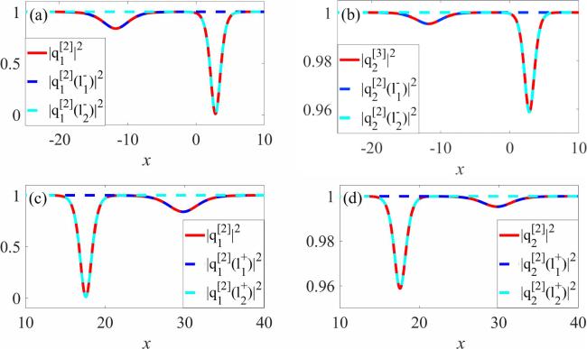
Figure 5. The collision dynamics of two SVDSs. Left panels: dynamical evolution of dark soliton solution $| {q}_{1}^{[2]}{| }^{2}$ before (t = −2, (a)) and after (t = 10, (c)) the collision. Right panels: dynamical evolution of dark soliton solution $| {q}_{2}^{[2]}{| }^{2}$ before (t = −2, (b)) and after (t = 10, (d)) the collision. The solid red line describes the evolution of the dark soliton solution (9) with ns = 2, nd = 0. The blue line and green line show the evolution of the solution (24) along the trajectory l1 and the trajectory l2, respectively. The relevant parameters are consistent with those selected in figure 1.
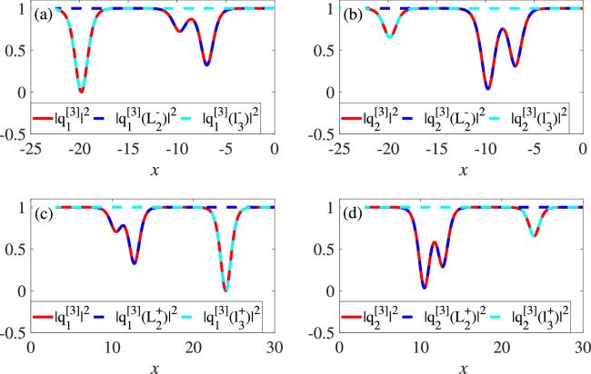
Figure 6. The collision dynamics of an SVDS and a DVDS. Left panels: dynamical evolution of dark soliton solution $| {q}_{1}^{[3]}{| }^{2}$ before (t = − 3, (a)) and after (t = 5, (c)) the collision. Right panels: dynamical evolution of dark soliton solution $| {q}_{2}^{[3]}{| }^{2}$ before (t = −3, (b)) and after (t = 5, (d)) the collision. The solid red line describes the evolution of the dark soliton solution (9) with ns = 1, nd = 1. The blue line shows the evolution of the solution (30) along the trajectory L2. The green line shows the evolution of the solution (24) along the trajectory l3. The analysis suggests that the collisions for SVDSs are always elastic, whereas the collision of DVDSs can be inelastic. The parameters are c = (−0.1,0.7, −0.7, −0.8, 2, 5, −0.1−1.1662i, 0.1246−1.1093i, −0.2942 + 1.1603i), a1 = 1, a2 = −0.6, c1 = 1, c2 = 1, and α = 0.5.
In fact, a plethora of experimental evidence has demonstrated that inelastic collisions occur in most cases for DVDSs, which is consistent with the outcomes we discussed in theorem 2. For example, the two DVDSs in figure 7 do not keep their pre-collision shape after the collision implying that they both exhibit inelastic collisions.
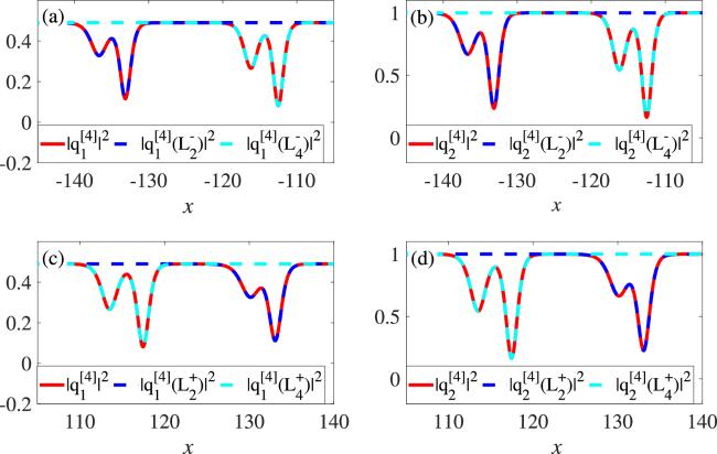
Figure 7. The collision dynamics of two DVDSs. Left panels: dynamical evolution of multi-dark soliton solution $| {q}_{1}^{[4]}{| }^{2}$ before (t = −50, (a)) and after (t = 50, (c)) the collision. Right panels: dynamical evolution of dark soliton solution $| {q}_{2}^{[4]}{| }^{2}$ before (t = −50, (b)) and after (t = 50, (d)) the collision. The solid red line describes the evolution of the dark soliton solution (9) with ns = 0, nd = 2. The blue line shows the evolution of the solution (30) along the trajectory L2. The green line shows the evolution of the solution (30) along the trajectory L4. The collisions of DVDSs are obviously inelastic. The parameters are a1 = −0.6, a2 = −0.6, c1 = 0.7, c2 = 1, α = 0.5, and c = (−0.9, −0.7, −0.6, 2, 5.2, 5, −0.5, 0.3–1.0630i, 0.3–0.7i, 0.3–0.8246i, 0.3–1.1136i).
In light of this, we proceed to ascertain the conditions that give rise to elastic behavior in collisions for DVDSs. It should be highlighted that the asymptotic expression of a DVDS before and after the collision differs primarily in terms of the phase shift. Thus, the collision is elastic if the phase differences of the two valleys of the DVDS are equal before and after the collision; otherwise, it is inelastic. From the asymptotic expressions (30) we can also derive the elastic condition for the DVDSs as follows:
$\begin{eqnarray}\left\{\begin{array}{l}{\prod }_{l=1}^{j-2}{\left|\displaystyle \frac{{\chi }_{l}-{\chi }_{j}}{{\chi }_{l}-{\chi }_{j-1}}\right|}^{2}=\displaystyle \prod _{l=j+1}^{n}{\left|\displaystyle \frac{{\chi }_{l}-{\chi }_{j}}{{\chi }_{l}-{\chi }_{j-1}}\right|}^{2},\\ {\prod }_{l=1}^{j-2}{\left|\displaystyle \frac{{\chi }_{l}^{* }-{\chi }_{j}}{{\chi }_{l}^{* }-{\chi }_{j-1}}\right|}^{2}=\displaystyle \prod _{l=j+1}^{n}{\left|\displaystyle \frac{{\chi }_{l}^{* }-{\chi }_{j}}{{\chi }_{l}^{* }-{\chi }_{j-1}}\right|}^{2},\end{array}\right.\end{eqnarray}$
where χl is defined in equation (10). Different from figure 6, the two valleys of the DVDS in figure 8 are separated by a relatively wide distance (the displacement difference between the two valleys before and after the collision of the DVDS is much smaller than the initial distance of the two valleys). The interaction between the two valleys is extremely weak in this case, so even if the DVDS in figure 8 has an inelastic collision, the shape change after the collision is easily ignored.
Figure 8. The collision dynamics of an SVDS and a DVDS. Left panels: Dynamical evolution of a multi-dark soliton solution $| {q}_{1}^{[3]}{| }^{2}$ before (t = −1, (a)) and after (t = 6, (c)) the collision. Right panels: dynamical evolution of a multi-dark soliton solution $| {q}_{2}^{[3]}{| }^{2}$ before (t = −1, (b)) and after (t = 6, (d)) the collision. The solid red line describes the evolution of the dark soliton solution (9) with ns = 1, nd = 1. The blue line shows the evolution of the solution (30) along the trajectory L2. The green line shows the evolution of the solution (24) along the trajectory l3. The profile of the DVDS changes too slightly to be visible after the collision at these parameters. The parameters are the same as in figure 3.

4. Conclusions

In summary, we provide a sufficient condition for the existence of dark soliton solutions and proceed to derive the uniform expressions of such solutions including both SVDSs and DVDSs by means of the uniform Darboux transformation. The analysis indicates that while elastic collisions are a common feature of SVDSs, inelastic collisions are prevalent in most instances for DVDSs. Notably, we also propose a condition that guarantees elastic collisions for DVDSs. The dark soliton solutions derived from the defocusing coupled Hirota equation possess the potential for applications in physical fields such as signal transmission and modulation in the realm of fiber optic communication [32, 45]. Furthermore, our results also shed new light on the fundamental properties of dark solitons, and may provide a promising avenue for future research in the fields of nonlinear optics and photonics [46, 47].

Liming Ling is supported by the National Natural Science Foundation of China (No. 12 122 105).

1
Haus H A Wong W S 1996 Solitons in optical communications Rev. Mod. Phys. 68 423 444

DOI

2
Kivshar Y S Agrawal G P 2003 Optical Solitons: From Fibers to Photonic Crystals Academic Press

DOI

3
Peregrine D H 1983 Water waves, nonlinear Schrödinger equations and their solutions ANZIAM J. B 25 16 43

DOI

4
Benney D J Newell A C 1967 The propagation of nonlinear wave envelopes Stud. Appl. Math. 46 133 139

DOI

5
Shukla P K Eliasson B 2010 Nonlinear aspects of quantum plasma physics Phys. Usp. 53 51 76

DOI

6
Dalfovo F Giorgini S Pitaevskii L P Stringari S 1999 Theory of Bose–Einstein condensation in trapped gases Rev. Mod. Phys. 71 463 512

DOI

7
Agrawal G P 2000 Nonlinear Fiber Optics Nonlinear Science at the Dawn of the 21st Century Heidelberg Springer, Berlin 195 211

DOI

8
Kim J Park Q H Shin H J 1998 Conservation laws in higher-order nonlinear Schrödinger, equations Phys. Rev. E 58 6746 6751

DOI

9
Nakkeeran K 2002 Bright and dark optical solitons in fiber media with higher-order effects Chaos Solit. Fractals 13 673 679

DOI

10
Hirota R 1973 Exact envelope-soliton solutions of a nonlinear wave equation J. Math. Phys. 14 805 809

DOI

11
Tasgal R S Potasek M J 1992 Soliton solutions to coupled higher-order nonlinear Schrödinger equations J. Math. Phys. 33 1208 1215

DOI

12
Hasegawa A Kodama Y Maruta A 1997 Recent progress in dispersion-managed soliton transmission technologies Opt. Fiber. Technol. 3 197 213

DOI

13
Kang Z Z Xia T C 2019 Construction of Multi-soliton solutions of the N-coupled Hirota Equations in an optical fiber* Chinese Phys. Lett. 36 110201

DOI

14
Ankiewicz A Soto-Crespo J M Akhmediev N 2010 Rogue waves and rational solutions of the Hirota equation Phys. Rev. E 81 046602

DOI

15
Tao Y S He J S 2012 Multisolitons, breathers, and rogue waves for the Hirota equation generated by the Darboux transformation Phys. Rev. E 85 026601

DOI

16
Wang D S Chen F Wen X Y 2016 Darboux transformation of the general Hirota equation: multisoliton solutions, breather solutions, and rogue wave solutions Adv. Differ. Equ. 2016 1 17

DOI

17
Chen S Y Yan Z Y 2019 The Hirota equation: Darboux transform of the Riemann–Hilbert problem and higher-order rogue waves Appl. Math. Lett. 95 65 71

DOI

18
Chowdury A Ankiewicz A Akhmediev N 2015 Moving breathers and breather-to-soliton conversions for the Hirota equation Proc. R. Soc. A: Math. Phys. Eng. Sci. A 471 20150130

DOI

19
Zhang H Q Yuan S S 2017 Dark soliton solutions of the defocusing Hirota equation by the binary Darboux transformation Nonlinear Dyn. 89 531 538

DOI

20
Zhang X E Ling L M 2021 Asymptotic analysis of high-order solitons for the Hirota equation Phys. D: Nonlinear Phenom. 426 132982

DOI

21
Zhang X M Qin Y H Ling L M Zhao L C 2021 Inelastic interaction of double-valley dark solitons for the Hirota equation Chinese Phys. Lett. 38 090201

DOI

22
Wang T Y Qin Z Y Mu G Zheng Z F 2023 General high-order rogue waves in the Hirota equation Appl. Math. Lett. 140 108571

DOI

23
Qin Y H Zhang X M Ling L M Zhao L C 2022 Phase characters of optical dark solitons with third-order dispersion and delayed nonlinear response Phys. Rev. E 106 024213

DOI

24
Yang D Y Tian B Qu Q X Zhang C R Chen S S Wei C C 2021 Lax pair, conservation laws, Darboux transformation and localized waves of a variable-coefficient coupled Hirota system in an inhomogeneous optical fiber Chaos Solit. Fractals 150 110487

DOI

25
Zhang G Q Yan Z Y Wen X Y Chen Y 2017 Interactions of localized wave structures and dynamics in the defocusing coupled nonlinear Schrödinger equations Phys. Rev. E 95 042201

DOI

26
Chen S H Song L Y 2013 Rogue waves in coupled Hirota systems Phys. Rev. E 87 032910

DOI

27
Qin Y H Zhao L C Yang Z Q Ling L M 2021 Multivalley dark solitons in multicomponent Bose–Einstein condensates with repulsive interactions Phys. Rev. E 104 014201

DOI

28
Park Q H Shin H J 2000 Higher order nonlinear optical effects on polarized dark solitons Opt. Commun. 178 233 244

DOI

29
Nakkeeran K 2001 Exact dark soliton solutions for a family of N coupled nonlinear Schrödinger equations in optical fiber media Phys. Rev. E 64 046611

DOI

30
Huang X 2016 Rational solitary wave and rogue wave solutions in coupled defocusing Hirota equation Phys. Lett. A 380 2136 2141

DOI

31
Zhang H Q Yuan S S 2017 General N-dark vector soliton solution for multi-component defocusing Hirota system in optical fiber media Commun. Nonlinear Sci. Numer. Simul. 51 124 132

DOI

32
Bindu S G Mahalingam A Porsezian K 2001 Dark soliton solutions of the coupled Hirota equation in nonlinear fiber Phys. Lett. A 286 321 331

DOI

33
Chai H P Tian B Du Z 2018 The Nth-order Darboux transformation, vector dark solitons and breathers for the coupled defocusing Hirota system in a birefringent nonlinear fiber Chinese J. Phys. 56 2241 2253

DOI

34
Peng W Q Tian S F Wang X B Zhang T T 2020 Characteristics of rogue waves on a periodic background for the Hirota equation Wave Motion 93 102454

DOI

35
Du Z Xu T Ren S 2021 Interactions of the vector breathers for the coupled Hirota system with 4 × 4 Lax pair Nonlinear Dyn. 104 683 689

DOI

36
Nisar K S Inan I E Martinez H Y Inc M 2022 Some new type optical and the other soliton solutions of coupled nonlinear Hirota equation Results Phys. 35 105388

DOI

37
Sun W R Wang L 2020 Solitons, breathers and rogue waves of the coupled Hirota system with 4 × 4 Lax pair Commun. Nonlinear Sci. Numer. Simul. 82 105055

DOI

38
Xu H X Yang Z Y Zhao L C Duan L Yang W L 2018 Breathers and solitons on two different backgrounds in a generalized coupled Hirota system with four wave mixing Phys. Lett. A 382 1738 1744

DOI

39
Zhao H H Zhao X J Hao H Q 2016 Breather-to-soliton conversions and nonlinear wave interactions in a coupled Hirota system Appl. Math. Lett. 61 8 12

DOI

40
Xie X Y Liu X B 2020 Elastic and inelastic collisions of the semirational solutions for the coupled Hirota equations in a birefringent fiber Appl. Math. Lett. 105 106291

DOI

41
Yu W T Luan Z T Zhang H X Liu W J 2022 Collisions of three higher order dark double-and single-hump solitons in optical fiber Chaos Solit. Fractals 157 111816

DOI

42
Ma G L Zhou Q Yu W T Biswas A Liu W J 2021 Stable transmission characteristics of double-hump solitons for the coupled Manakov equations in fiber lasers Nonlinear Dyn. 106 2509 2514

DOI

43
Ling L M Zhao L C Guo B L 2015 Darboux transformation and multi-dark soliton for N-component nonlinear Schrödinger equations Nonlinearity 28 3243

DOI

44
Faddeev L D Takhtajan L A 1987 Hamiltonian Methods in The Theory of Solitons Springer

DOI

45
Sun W R Tian B Wang Y F Zhen H L 2015 Dark single-and double-hump vector solitons of the coupled higher-order nonlinear Schrödinger equations in the birefringent or two-mode fibers Opt. Commun. 335 237 244

DOI

46
Zhou Q Xu M Y Sun Y Z Zhong Y Mirzazadeh M 2022 Generation and transformation of dark solitons, anti-dark solitons and dark double-hump solitons Nonlinear Dyn. 110 1747 1752

DOI

47
Musammil N M Subha P A Nithyanandan K 2019 Phase dynamics of inhomogeneous Manakov vector solitons Phys. Rev. E 100 012213

DOI

Outlines

/