


1. Introduction
In the past few decades, cold atoms and molecules have been tamed by inhomogeneous magnetic field in various ways, such as Zeeman decelerator [1–4], magnetic guide [5, 6], magnetic mirror [7], magnetic storage ring [8], magnetic conveyor belt [9, 10], magnetic beam splitter [11–14], atomic interferometer [15–17], magnetic trap [18–23], and so on. Most magnetic traps are designed for atoms and molecules in weak-field-seeking states which are not the lowest-energy configurations. Therefore, the captured atoms and molecules may escape from the trap due to inelastic collisions which is harmful for the evaporative or sympathetic cooling. However, the trap loss can be circumvented in the ground state. It is worth noting that the ground state of any molecule is strong-field seeking. Once the external field is sufficiently strong, all molecules become strong-field seekers. Furthermore, all states of heavy molecules having small rotational constants become strong-field-seeking even in small magnetic fields. Obviously, the trapping of molecules in a strong-field-seeking state is important and meaningful. Unfortunately, the creation of a magnetostatic maximum in free space is impossible according to Maxwell's equations and Earnshaw's theory. Therefore, a time-dependent magnetic field is required. The first AC magnetic trap for neutral atoms was demonstrated by E A Cornell et al [24]. The dynamic trap was made by passing an alternating current through circular wires located with their axis parallel to a uniform static magnetic field. During one cycle, the atoms were first focused axially and expelled radially, and then they were expelled axially and focused radially. Wang's group proposed an AC magnetic trap [25] for cold atoms. The trap was composed of four Ioffe bars and a pair of Helmholtz coils. An AC quadrupole magnetic field and a DC bias field were generated by the Ioffe bars and the Helmholtz coils, respectively. In this paper, we propose a much simpler AC magnetic trap. Our trap can be combined with the mature technology of Zeeman slowly, and easily realized in the experiment. The paper is organized as follows. The schematic diagram of our AC trap is depicted first. The time-sequential control and the distribution of the magnetic field are given. We investigate how the switching frequency and the electric current in the coils impact the number of trapped molecules. Then we study the variation of the locations and phase-space distribution in a whole switching cycle. Finally, we add the ‘free-fly time' into the switching sequence, and study its influence on the trapped molecules.
2. The scheme of our AC magnetic trap
2.1. Schematic diagram
As depicted in figure 1, our trap is composed of two pairs of Helmholtz coils. Four racetrack-shaped coils are of the same size. The length and width of each coil are a and b, respectively. The distance between two parallel coils is d. The two ends of each coil are semicircular with a radius of r. Here, a = 16 mm, b = 7 mm, d = 10 mm, r = 3.5 mm. Previous magnetic traps need a magneto-optical trap (MOT) to obtain cold atoms. Thanks to the development of Zeeman deceleration of paramagnetic molecules, our AC trap can be combined with the Zeeman slower.

Figure 1. The schematic diagram of our AC magnetic trap. The dimensions of the coils and the distance between the two coils are indicated in the inset on the right. |
2.2. Time-sequence control
As the formation of a magnetostatic maximum in free space is impossible, we design an AC magnetic trap. As shown in figure 2, we alternately switch the current flowing through the coils. T is the switching cycle, Ty and Tz are the duration of applying current in the coils along the Y-axis (green arrow in figure 1) and Z-axis (blue arrow in figure 1), respectively. When currents in the coils along the Y-axis are switched on, the magnetic field intensity at the center is maximum along the Z-axis and minimum along the Y-axis. As the molecules are in the strong-field-seeking state, they are attracted to the center along Z-axis while repelled from the center along Y-axis. On the contrary, while currents in the coils along the Z-axis are switched on, the molecules are attracted to the center along the Y-axis while they are repelled from the center along the Z-axis. Along the X-axis, there is always the strongest magnetic field intensity at the center. The focusing and defocusing directions are periodically reversed, and the molecules feel a net focusing toward the center.
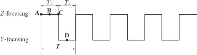
Figure 2. Time-sequence control diagram indicates the focusing situation at different time. Points (A), (B), (C), and (D)indicate four special moments during the 61st switching cycle. |
Four moments during the 61st switching cycle are marked as A, B, C, and D in figure 2. The four moments are 60 T, 60.25 T, 60.5 T and 60.75 T, respectively.
2.3. The magnetic field distribution
Each coil is made up of four turns of copper wires. The current that flows through each wire is I0. Here we set I0 as 1500 A. As is depicted in figure 3, the distribution of the magnetic field is calculated numerically with commercial software (Comsol Multiphysics). The label is in unit of Tesla (T). First, we turn on the currents in the coils along the Y-axis. As is shown in figures 3(a)–(c), the magnetic field intensity at the center is minimum along the Y-axis and maximum in the XZ plane.
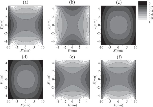
Figure 3. The contour map of the magnetic field (unit: Tesla) for the Y-defocusing (a)–(c) and Z-defocusing (d)–(f) configurations. |
The molecules in the strong-field-seeking state will be attracted to the center in the XZ plane and repelled from the center along the Y-axis. As is indicated in figures 3(d)–(f), the magnetic field intensity at the center is maximum in the XY plane and minimum along the Z-axis. This time the molecules will be attracted to the center in the XY plane and repelled from the center along the Z-axis. We need to switch the two modes at an appropriate frequency to trap the molecules efficiently.
3. The Monte Carlo simulations
To test the performance of our AC trap, we numerically simulate the dynamic process of trapping molecules using the classical Monte Carlo method. We choose OH radical as our test molecule. The main reasons are listed as follows: on the one hand, many mature methods have been used to produce the OH molecular beam, such as pulsed discharge [26] and photodissociation [27]. On the other hand, the OH radical has been successfully decelerated by the Stark decelerator [27] and the Zeeman slower [28]. In the following simulation, we choose the OH molecules that are populated in the lowest rotational level of the vibrational state (v = 0) and electronic ground state (X2 Π3/2).
We first operate our AC trap in the conventional switching mode in section 3.1 . To further efficiently trap the molecules, we attempt to optimize the switching mode in section 3.2 . The numbers of molecules for the simulations (figures 4–6, 10) are 100 thousand and 1 million (figures 7–8), respectively. The initial distributions of the locations and velocities of molecules are Gaussian. The initial molecular beam centered at X = Y = Z = 0, Vx = Vy = Vz = 0. The full width at half-maximum of the position and velocity distributions are ΔX = 1 mm, ΔY = 1 mm, ΔZ = 1 mm, and ΔVx = 10 m s−1, ΔVy = 10 m s−1, ΔVz = 10 m s−1, respectively. As is shown in figure 1, the molecular beam is slowed by the decelerator first. Then we need to create an energy barrier to further slow the molecules [29–31]. After the molecules reach the center, they have already been decelerated to near a standstill. At this time, our AC trap began to work. In this paper, we put emphasis on the performance of our AC trap and haven't simulated the process of loading OH molecules into the trap.
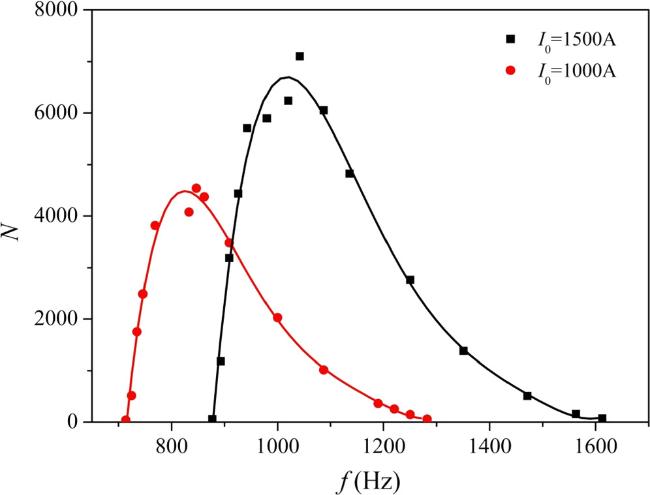
Figure 4. The number of trapped molecules versus the switching frequency. The squares and circles show the current values are 1500 A and 1000 A, respectively. The solid lines are fitting curves. |

Figure 5. The frequency corresponding to the maximum number of trapped molecules as a function of the current intensity. |

Figure 6. The number of trapped molecules as a function of the time (Ty) during which the coils along the y-axis are energized. The switching cycle is 820 μs and the current is 2000 A. For each Ty , the maximum number of trapped molecules is chosen. |
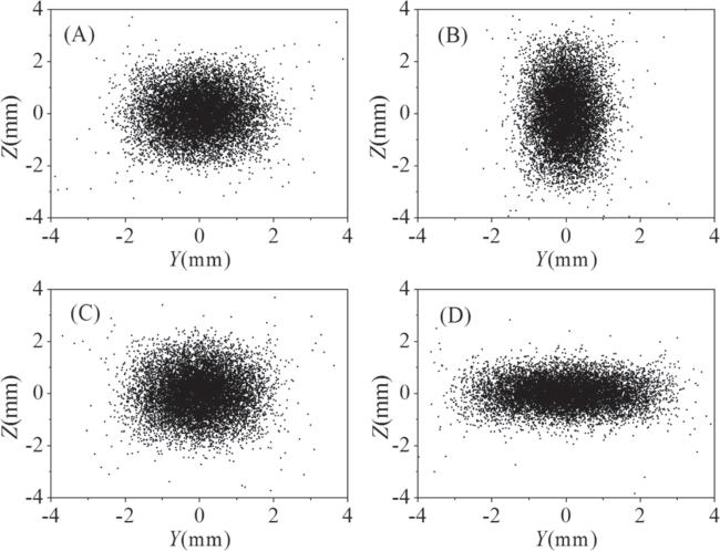
Figure 7. The distribution of molecules at four different moments within the 61st switching cycle at a switching frequency of 1220 Hz. The four moments (A, B, C, D) are indicated in figure 2. |
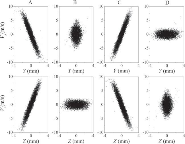
Figure 8. The phase-space distribution of trapped molecules at four different moments within the 61st switching cycle with the switching frequency of 1220 Hz. |
3.1. The conventional switching mode
The time sequence diagram is depicted in figure 2. The currents in the coils along the Y-axis and Z-axis are switched on and off alternately. Here, Ty = Tz = 0.5 T, and f = 1/T. The number of trapped molecules versus the switching frequency (f) after a 100 ms trapping time is indicated in figure 4. Two different values of currents (I0) are used. The black squares and the red circles indicate that the simulation data for I0 are equal to 1500 A and 1000 A, respectively. From figure 4, we can see that there is always an appropriate switching frequency corresponding to the maximum number of trap molecules. We need to switch the current frequently to let the molecules feel a net force [32]. If the switching frequency is too low, the molecules will be lost along the defocusing direction. However, if we switch the current too frequently, the micromotion of the molecule becomes smaller and faster and the net force towards the trap center vanishes [33]. The maximum number of trap molecules for I0 = 1500 A is much larger compared to the case for I0 = 1000 A. For the higher current, trapping works in a range between 877 and 1613 Hz. For the lower current, trapping works in a relatively narrow range between 714 and 1282 Hz. The optimal switching frequencies for I0 = 1500 A and 1000 A are 1042 Hz and 847 Hz, respectively. The optimal frequency shifts to a higher value for a larger current.
In addition, we study the relationship between the switching frequency and the current. For each current, we get an optimized switching frequency corresponding to the maximum number of trapped molecules.
Considering the experimental feasibility, we can hardly apply too high current. For the current range in our simulation, we find that the larger the current is, the larger the switching frequency is. This can be explained as follows: Paramagnetic molecules feel a dipole gradient force in an inhomogeneous magnetic field. The molecules in the strong-field-seeking state are defocused in one direction and focused in the other two directions. The larger the current is, the stronger the force is. A larger force will make the molecules move much faster, so we need to change the current more frequently.
In the above discussions, we maintain Ty equal to Tz. Now, we keep T equal to 820 μs unchanged and vary Ty to see how the number of trapped molecules is affected. As shown in figure 6, the number of trapped molecules is maximum when Ty is equal to Tz. The greater the difference between Ty and Tz is, the fewer molecules can be trapped. These can be attributed to the good symmetry of our AC magnetic trap about the X-axis.
To better understand the performance of our trap, we investigate the molecular distribution at different moments within the 61st switching cycle. The four sub-graphs represent the distribution of trapped molecules in the YZ plane at four different moments indicated in figure 2. Here, Ty = Tz = 410 μs, T = Ty+Tz, I0 = 2000 A. In figure 7(A), the molecules have just experienced Y-focusing and they are moving outward along the Z-axis and inward along the Y-axis. As shown in figure 7(B), in the middle of Z-focusing, the molecular cloud is focused in the Y-axis and elongated in the Z-axis. This is a turning point before the molecules change their direction of motion. Then the molecules move inward along the Z-axis and outward along the Y-axis. Therefore, the shape of the molecular cloud in figure 7(C) is round which is similar to the case of figure 7(A). The Y-focusing forces have decelerated the motion along both Y-axis and Z-axis. Moment D is also a turning point, contrary to the case in figure 7(B), the molecular cloud is elongated in the Y-axis and focused in the Z-axis.
The variation of the phase-space distributions during the 61st switching cycle is depicted in figure 8. In the first row, Vy is plotted versus Y, and Vz is plotted versus Z in the second row. The four capital letters for each column indicate four moments within the 61st switching cycle marked in figure 2.
The distribution oscillates in both position and velocity. As illustrated in figure 8, the distribution rotates clockwise from A to D. The opposite phase-space distribution between the first and second lines is caused by the time delay of half a switching cycle. The spread in position along the Y(Z)-axis is minimal in the middle of the Z(Y)-focusing stage. In contrast, the spread in velocity along the Y(Z)-axis is minimum in the middle of the Y(Z)-focusing stage.
3.2. The optimized switching mode
In this section, we explore how to optimize the switching mode. Unlike the conventional switching mode, we switch off the current after a Y(or Z)-focusing stage. Once the current is switched off, the molecules fly freely because they no longer feel the magnetic gradient force. As illustrated in figure 9, the switching cycle is the sum of Ty, Tz, and Toff.
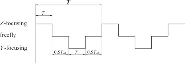
Figure 9. The switching diagram that indicates the focusing situation and switching off the current at different time. |
We study the number of trapped molecules(N) versus the duration of the Y-focusing and Z-focusing stages (Ton) for different values of time for which the current is turned off(Toff). I0 is set as 2000 A, Toff is varied from 0 to 800 μs with an interval of 200 μs.
We can conclude from figure 10 that the conventional switching mode (Toff = 0) is not the best choice. For each curve, once the Toff is determined, there is always an appropriate Ton corresponding to the maximum number of trapped molecules. The appropriate Ton for Toff = 0, 200, 400, 600, 800 μs are 820, 640, 500, 440, and 360 μs, respectively. As Toff increases, the optimized Ton shifts to smaller values, and the maximum number of trapped molecules first increases then decreases.

Figure 10. The number of molecules as a function of the time during which the focusing and defocusing fields are switched on. The black square, red circle, green triangle, blue triangle, and cyan diamond represent the values of Toff are 0, 200 μs, 400 μs, 600 μs, and 800 μs, respectively. |
4. Conclusions
In this paper, an AC magnetic trap composed of two pairs of Helmholtz coils is proposed. We operate the trap in two different modes. With the help of commercial finite element software, we calculate the distribution of magnetic fields numerically. In the conventional mode, we investigate the influence of the switching frequency and the electric current in the coils on the number of trapped molecules. We find that there is always an optimized switching frequency corresponding to the maximum number of trapped molecules. The larger the current is, the higher the optimized switching frequency is. We investigate the influence of the difference between Ty and Tz on the trapping efficiency. We conclude that when Ty equals Tz, our AC trap works best. We also simulate the variation of the locations and the phase-space distribution in a whole switching cycle. We infer that the spread in position along the Y(Z)-axis is minimum in the middle of the Z(Y)-focusing stage. Meanwhile, the spread in velocity along Y(Z)-axis is minimal in the middle of the Y(Z)-focusing stage. Finally, we explore how to optimize the switching mode. We add Toff to a switching cycle. We find that as Toff increases, the optimized Ton decreases and the maximum number of trapped molecules first increases and then decreases.