


1. Introduction
In dissipative systems, numerous natural processes are characterized by a large number of coexisting attractors rather than a single long term asymptotic state or attractor for a given set of parameters. This phenomenon is well-known as multistability [1]. Studies on multistable systems are interdisciplinary and have gained attention in various fields of science such as neuroscience [2], lasers and optics [3], condensed matter physics [4], chemistry [5, 6], rheology [7], nuclear physics [8], ecology [9], fluid-dynamics [10, 11], semiconductor physics [12] and biology [13]. Experimental and theoretical models have revealed distinct paths to multistability in various systems such as weakly dissipative systems [14], coupled systems [15], delayed feedback systems [16], parametrically excited systems [17], and stochastic systems [18].
The occurrence of multiple attractors is often determined by the system class such as dissipation strength, coupling type and intensity, time delay, amplitude and frequency of parameter perturbation, nature of external forcing and noise intensity [17, 19]. These system components have been shown to influence several nonlinear phenomena observed in multistable systems including synchronization, memory capability mechanism in artificial neural networks, absolute negative mobility and current reversal, hidden and self-excited attractors, chaos and nonlinear resonance [20–24]. A much studied type of nonlinear resonance observed in multistable systems with weak signal generated by applying white noise to an external signal with a broad frequency range is the stochastic resonance (SR) [25]. The frequencies in the white noise that correlate to the frequencies in the original signal will resonate with each other, amplifying the original signal and thereby increasing the signal-to-noise ratio, which makes the original signal more prominent. A similar phenomenon to the well-known SR that is recently gaining research attention is vibrational resonance (VR). In VR, the noise term is replaced by a variable high-frequency force [26]. Because it is easier to engineer deterministic systems than noise-driven systems, several applications of VR have been proposed. Notable among these applications are found in the detection, isolation, amplification and transmission of weak periodic, aperiodic and random signals [27–29], bearings fault diagnosis [30, 31], improving electrical power harvesting from environmental kinetic energy [32, 33], the induction of set-reset logic gates and other memory devices [34, 35], nano-electromechanical resonator [36], and very recently in thermo-optic optomechanical nanocavity [37].
Vibrational resonance has been observed in different systems with different potentials distribution, such as the monostable potential, bistable potential and multistable potential. The choice of dissipative multistable potential for studies on VR is encouraged because chaotic attractors are rarely found in weakly dissipative multistable systems close to the conservative limit [1]. We note that there has been considerable growth in literature on VR in multistable systems, which includes studies on VR in ratchet [38], Josephson junctions, plasmas, phase-locked loops, or pendulums [39, 40] and gyroscope [41]. In most of these studies, the prominent phenomenon is multiresonance [20, 42–44].
However, the effect of other system parameters and consequential inherent topological changes on the observed multiresonance has motivated further attention. For instance, Yang and Liu [44] showed that the delay term effectively controls multiresonance in a delayed multistable system. Similarly, Rajasekar et al [43] observed that the bifurcation of equilibrium points takes place at resonance in a multistable system with symmetric potential. Chizhevsky [20] demonstrated experimental evidence of the phenomenon of vibrational resonance in a vertical-cavity surface-emitting laser (VCSEL) operating in the regime of polarization multistability by producing a series of resonances on the low frequency influenced by the high-frequency (HF) amplitude reminiscent of multiresonance. Roy-Layinde et al [39] reported that frictional inhomogeneity controls the appearance of VR in a driven multistable oscillator with symmetric potential. In fractional-order overdamped systems, the arbitrary (non-integer) order provokes richer resonance features in comparison to conventional integer order [42]. The deformation parameter significantly modulates the resonance peaks observed for a particle placed in a nonlinear deformable asymmetrical Remoissenet–Peyrard potential [40]. Most of the system parameters has received a lot of attention, however, one of the less scrutinized parameters is the inertial mass. A recent study showed that constant inertial mass complements the role of bi-harmonic forcing with two distinct behaviours characterizing the occurrence of VR [45]. However, many real systems exist for which a fixed constant mass is not a good representation because their effective mass undergoes monotonic changes during dynamical time or position evolution which manifest as varying mass as found in for instance, alteration of the mass of products on the conveyor belt during loading and unloading processes in a rotor-conveyor belt system, and during the motion of a falling meteorite.
When the mass explicitly depends on the position, it is called position-dependent mass (PDM). Nonlinear phenomena in systems with variable mass may differ significantly from those with constant mass [46, 47]. For instance, the resonant state might be altered by mass variation as highlighted in our recent papers [48, 49]. The nature and mechanism of resonance behaviour are yet to be fully understood. The variable mass parameters were recently shown to influence VR in a biharmonically-driven PDM oscillator modelling the inversion of NH3 molecule by driving the system from single to double resonance state [48]. Since it has been suggested that VR could be optimally explored in the control of the motion of tiny particles in nanoscience or microscale/macroscale oscillators [48–50], studies on the influence of particle mass variation on resonances will unravel certain features of systems modelled by variable mass functions. In practical applications, the variable mass efficiently re-tunes the frequency of a feasible adaptive-passive variable mass tuned mass damper (APVMTMD) with minimal power consumption, and no manual operations [51]. The variable mass-tuned vibration absorber (VMTVA) which possesses natural frequency that can be adjusted by changing its mass has been implemented as a generalized control strategy to reduce the resonance of a primary system [52]. In addition, it was recently shown that minute variation of mass can significantly impact on the bifurcation voltage of coupled vibrating piezoelectric L-shaped resonator, thereby enabling the detection of micro-mass [53]. In addition, research on PDM has enriched the understanding of a wide range of physical and optical properties of solid materials, such as semiconductors [54], crystalline and helium structures [55] quantum fluids [56], quantum wells and quantum dots [57], to mention but a few. Consequently, the influence of the variable mass parameters could be leveraged to maximize the effectiveness of devices used in VR modes. Hence, it will be insightful to investigate the impacts of PDM on the resonant state for different systems, particularly in a multistable system as recently presented for PDM bistable systems [49].
In this paper, we will explore the role of PDM parameters on VR phenomenon in a multistable system modelling one-dimensional motion of a single particle with spatially varying mass, symmetric potential and space-dependent damping. Our results could provide more insight into the vibrational modes of nanoparticles and spectroscopy of a wider range of systems with variable mass. The subsequent sections of this paper are arranged in the following order: In section 2 , we introduce the multistable system under investigation. In section 3 , we present the numerical analyses of the response amplitude. Section 4 contains the analytical procedure for the computation of the response amplitude, and Section 5 contains the results and discussion of our findings. Lastly, in section 6 , we summarize the paper and conclude with brief discussions on some important applications of our findings.
2. The model
The generalized Newton's second law of motion for the classical PDM systems described by the Lagrangian function
$\begin{eqnarray}L(x,\dot{x};t)=T-V(x)=\displaystyle \frac{1}{2}m(x){\dot{x}}^{2}-V(x),\end{eqnarray}$
which satisfies the Euler–Lagrange equation $\begin{eqnarray}\frac{{\rm{d}}}{{\rm{d}}t}\left(\frac{\partial L}{\partial \dot{x}}\right)-\frac{\partial L}{\partial x}={F}_{N},\end{eqnarray}$
is given by $\begin{eqnarray}F(x,\dot{x};t)=F(x;t)+{R}_{\mathrm{PDM}}(x,\dot{x};t)=-\frac{{\rm{d}}V(x)}{{\rm{d}}x}+{F}_{N},\end{eqnarray}$
where the overdot denotes differentiation with respect to time. $T=\tfrac{1}{2}m(x){\dot{x}}^{2}$ and V(x) represent the kinetic and potential energies of the system, FN is the net dissipative force, F(x; t) is the system's inertial force and ${R}_{\mathrm{PDM}}(x,\dot{x},t)$ is a reactive force, which is a quadratic function of velocity due to the mass variation [58, 59].When a single particle with a differentiable and integrable variable mass m(x) driven by a force field moves deterministically in a uniform friction media with finite arbitrary potential V(x), one can easily show that the general force equation (3 ) describing the dissipative oscillator can be written as
$\begin{eqnarray}m(x)\ddot{x}+\frac{1}{2}m^{\prime} (x){\dot{x}}^{2}+\gamma (x)\dot{x}+\frac{{\rm{d}}V(x)}{{\rm{d}}x}={F}_{{\rm{ext}}},\end{eqnarray}$
where the dissipative term $\phi =-\gamma (x)\dot{x}+{F}_{{\rm{ext}}}$ accounts for both the damping term $\gamma (x)\dot{x}$ with coefficient γ(x) and external forcing Fext. The inertial force is $F(x;t)=m(x)\ddot{x}$, and ${R}_{\mathrm{PDM}}(x,\dot{x},t)=\tfrac{1}{2}\tfrac{{\rm{d}}m(x)}{{\rm{d}}x}$ is the mass variation induced reactive force correction to the Newton's equation for the analogous constant-mass vibrating particle [60, 61]. In this paper, we consider the motion of a one-dimensional massive PDM particle in a periodic heterogeneous lattice and in a medium with a material density profile created by a stationary pressure wave, where the analogous mechanical system has an inhomogeneous damping coefficient of the form $\begin{eqnarray}\gamma (x)={\gamma }_{0}[1-\lambda \sin ({kx}+\phi )],\end{eqnarray}$
and a symmetric potential with periodicity k given by [62, 63]: $\begin{eqnarray}V(x)=-\displaystyle \frac{{V}_{0}}{k}\cos {kx}.\end{eqnarray}$
The external forcing is a biharmonic driving signal consisting of additive dual-frequency signals given by $\begin{eqnarray}{F}_{{ext}}=f\cos \omega t+G\cos {\rm{\Omega }}t,\,\,\,\,({\rm{\Omega }}\gg \omega )\end{eqnarray}$
where $f\cos \omega t$ is a low-frequency periodic force and $G\cos {\rm{\Omega }}t$ is an added HF external signal.The equation (4 ) can be adapted to model the current flow through a Josephson junction with voltage and phase-dependent damping, which can be visualized as the unidirectional oscillatory motion of a particle subject to periodic varying damping (equation (5 )) trapped in a well of potential energy (equation (6 )). γ(x) is the ratio of the conductivities associated with the phase-coherent Cooper pairs and quasiparticle tunnelling. ${\gamma }_{0}=\nu {({\omega }_{j}{RC})}^{-1}$ is the friction coefficient, which is a function of the resistance R and capacitance C of the junction, and ωj is the Josephson frequency [64, 65].
The particle's variable mass distribution with fixed rest mass m0 and mass nonlinear strength a is defined by a regular mass function of the form [66]:9 ) has been studied in PDM harmonic oscillators [67].
$\begin{eqnarray}m(x)={m}_{0}{\left(1+{a}^{2}{x}^{2}\right)}^{\kappa },\,\,\,\,(a\geqslant 0),\end{eqnarray}$
where κ is a real variable, that determines the nature of a large family of PDM functions describing semiconductor heterostructures and impure crystalline materials. For the purpose of this work, we assume κ = −1, i.e. $\begin{eqnarray}m(x)=\displaystyle \frac{{m}_{0}}{1+{a}^{2}{x}^{2}},\,\,\,\,(a\geqslant 0).\end{eqnarray}$
Thus, m(x) is bounded without singularities, defined in the entire real line ${\text{}}{\text{}}D(m(x))\,\in \,{\mathfrak{R}}$, with a maximum $m{\left(x\right)}_{\max }={m}_{0}$ at x = 0, and m(x) vanishes as ∣x∣ → ∞ . The PDM function (By using the equations (5 )–(9 ) in the force equation (4 ), we can express the oscillator as a dissipative system of the form12 ) describes the multistable system with spatially varying mass otherwise referred to as a PDM mutltistable system under investigation. When the nonlinear strength vanishes (a = 0), the mass is independent of position and the system (equation (12 )) possesses constant mass as considered by Usama et al [45]. VR in a special case of equation (12 ) for a system with unitary mass (a = 0, m0 = 1) was examined by Roy-Layinde et al [39].
$\begin{eqnarray}\ddot{x}+b(x){\dot{x}}^{2}+c(x)\dot{x}+d(x)=h(x),\end{eqnarray}$
where $\begin{eqnarray}\begin{array}{rcl}b(x) & = & \frac{m^{\prime} (x)}{2m(x)}=-\frac{{a}^{2}x}{1+{a}^{2}{x}^{2}},\\ \,c(x) & = & \frac{\gamma (x)}{m(x)}=\frac{{\gamma }_{0}}{{m}_{0}}(1+{a}^{2}{x}^{2})[1-\lambda \sin ({kx}+\phi )],\\ d(x) & = & \frac{1}{m(x)}\frac{{\rm{d}}V(x)}{{\rm{d}}x}=\frac{{V}_{0}}{{m}_{0}}(1+{a}^{2}{x}^{2})\sin {kx},\\ h(x) & = & \frac{{F}_{{\rm{ext}}}}{m(x)}=\frac{(1+{a}^{2}{x}^{2})}{{m}_{0}}(f\cos \omega t+G\cos {\rm{\Omega }}t).\end{array}\end{eqnarray}$
Thus, the equation of motion of the biharmonically driven unidirectional particle with PDM, symmetric potential and position-dependent damping can be written as $\begin{eqnarray}\begin{array}{l}\ddot{x}-\displaystyle \frac{{a}^{2}x}{1+{a}^{2}{x}^{2}}{\dot{x}}^{2}+\displaystyle \frac{{V}_{0}}{{m}_{0}}(1+{a}^{2}{x}^{2})\sin {kx}\\ \quad +\displaystyle \frac{{\gamma }_{0}}{{m}_{0}}(1+{a}^{2}{x}^{2})[1-\lambda \sin ({kx}+\phi )]\dot{x}\\ \quad =\displaystyle \frac{(1+{a}^{2}{x}^{2})}{{m}_{0}}(f\cos \omega t+G\cos {\rm{\Omega }}t).\end{array}\end{eqnarray}$
Equation (From equation (12 ), it is evident that the variable mass effectively modified the original system potential (6 ) such that the modified potential becomes
$\begin{eqnarray}\begin{array}{rcl}V(x,a) & = & \left(\displaystyle \frac{{V}_{0}}{{m}_{0}{k}^{3}}\right)[[2{a}^{2}-{k}^{2}(1+{a}^{2}{x}^{2})]\cos {kx}\\ & & +2{a}^{2}k\sin {kx}].\end{array}\end{eqnarray}$
Hence, the variable mass impacts the system such that the particle effectively evolves in a deformable multistable potential comparable to the Remoissenet–Peyrardof substrate potential [68] of the form $\begin{eqnarray}V(x,a)=-\displaystyle \frac{{V}_{0}}{k}u(x,a)\cos {kx},\end{eqnarray}$
where u(x, a) is a perturbation function given by: $\begin{eqnarray*}u(x,a)=\left(\displaystyle \frac{1}{{m}_{0}{k}^{2}}\right)\left[[2{a}^{2}-{k}^{2}(1+{a}^{2}{x}^{2})]+2{a}^{2}k\tan {kx}\right].\end{eqnarray*}$
The maxima and minima of the potential are located at $\begin{eqnarray}x=\displaystyle \frac{n\pi }{k},\qquad n=0,\pm 1,\pm 2,\pm 3,\pm 4,\ldots .\end{eqnarray}$
For odd n, x is a minima, while for even n, x is a maxima.Since $\cos {kx}$ has a value of −1 at the minimum point, the depth (d) of the potential well (equation (14 )) below V(x) = 0 plane at the minima is given by
$\begin{eqnarray}d=\displaystyle \frac{{V}_{0}}{k}u(x,a).\end{eqnarray}$
Considering that $\tan {kx}=0$ at x = nπ/k, the depth of the well is $\begin{eqnarray}\begin{array}{rcl}d & = & \left|\displaystyle \frac{{V}_{0}}{{m}_{0}{k}^{3}}\left[2{a}^{2}-({k}^{2}+{a}^{2}{n}^{2}{\pi }^{2})\right]\right|,\\ n & = & \pm 1,\pm 3,\pm 5,\ldots .\end{array}\end{eqnarray}$
Consequently, the potential structure of the system is deformed by varying the nonlinear strength of the mass a. To get a clearer picture, we present the system's potential plot from equation (13 ) in figures 1(a) and (b) for four different values of the mass nonlinear strength a. Figure 1(a) depicts a symmetric periodic potential with periodicity k and potential barrier $\tfrac{{V}_{0}}{k}$ for PDM parameters (m0, a) = (1, 0) representative of equation (6 ). Clearly, the perturbed potential (13 ) is reduced to equation (6 )at a = 0, giving rise to the symmetry in the potential structure [39, 45]. However, increasing the value of a significantly yields three observable features on the potential structure of the multistable system as seen figure 1(b). First, it increases the amplitude of the potential. Secondly, it increases the depth of the potential well as we traverse along the x-axis through ∣x∣ > 0. This is shown in figure 2 for the variation of potential depth, d with nonlinear strength a. The depth of the potential well is computed from equation (17 ) with six values of nonlinear strength a (= 0, 0.03, 0.3, 0.5, 0.8, 1.0) in figure 2(a) and four values of number of wells n (= ±1, ±3, ±5, ±7) in figure 2(b). Lastly, it deforms the regular shape of the potential structure. It is worth mentioning that the potential structure of most nonlinear dynamical systems plays vital role in defining their dynamics, particularly, the resonance behaviour. Potential structures are crucial in predicting the resonance behaviour of nonlinear systems and could reveal vital parameters that could be employed to either enhance or suppress the occurrence of VR. These parameters include potential depth and well location [69, 70], and potential shape [40, 71, 72]. Therefore, it is important to critically scrutinize the effects of a varying mass, particularly the parameters of the PDM function on the dynamics and occurrence of VR in a nonlinear dissipative system as partly addressed by Usama et al [45]. Thus, the impact of the nonlinear strength of the mass on the occurrence of VR forms the crux of the analysis in this paper.
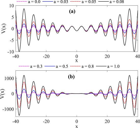
Figure 1. The effect of spatially varying mass on the system's potential structure computed from equation ( |
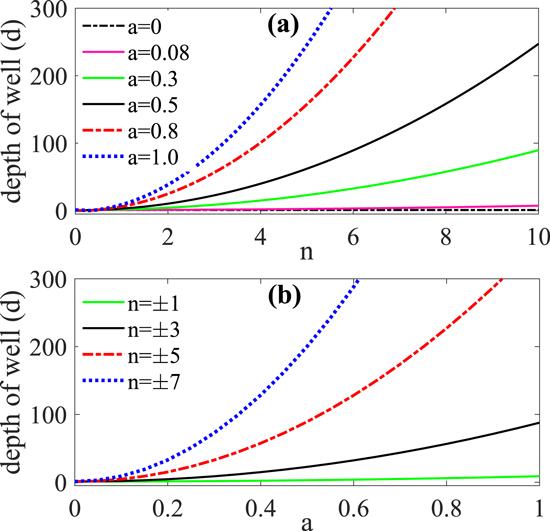
Figure 2. Variation of the depth of potential well, d computed from equation ( |
3. Numerical method
To compute the response amplitude Q which characterizes the system's response to the variation of the HF forcing at the low-frequency, it is usually convenient to write equation (12 ) as a set of coupled first-order autonomous ordinary differential equations (ODEs) of the form18 ) numerically for the output signal x(t) using the fourth order Runge-Kutta scheme, and compute the response amplitude Q from the Fourier spectrum of the time series of the variable x(t), such that
$\begin{eqnarray}\begin{array}{rcl}\frac{{\rm{d}}x}{{\rm{d}}t} & = & y,\\ \frac{{\rm{d}}y}{{\rm{d}}t} & = & \frac{{a}^{2}x}{1+{a}^{2}{x}^{2}}{y}^{2}-\frac{{V}_{0}}{{m}_{0}}(1+{a}^{2}{x}^{2})\sin {kx}\\ & & -\frac{{\gamma }_{0}}{{m}_{0}}(1+{a}^{2}{x}^{2})[1-\lambda \sin ({kx}+\phi )]y\\ & & +\frac{(1+{a}^{2}){x}^{2}}{{m}_{0}}(f\cos \omega t+G\cos {\rm{\Omega }}t).\end{array}\end{eqnarray}$
Next, we solve equation ( $\begin{eqnarray}\begin{array}{rcl}{A}_{S} & = & \frac{2}{{nT}}{\int }_{0}^{{nT}}x(t)\sin \omega t\,{\rm{d}}t,\\ {A}_{C} & = & \frac{2}{{nT}}{\int }_{0}^{{nT}}x(t)\cos \omega t\,{\rm{d}}t,\\ Q & = & \frac{\sqrt{{A}_{S}^{2}+{A}_{C}^{2}}}{f},\end{array}\end{eqnarray}$
where AS and AC are respectively the amplitudes of the sine and cosine components of the output signal computed at the frequency ω. $T=\tfrac{2\pi }{\omega }$ and n = (1, 2, 3,...) are respectively, the period of oscillation and the number of complete oscillations at the low-frequency input signal. The initial conditions used for all numerical computations are ($x(0)=0,\dot{x}(0)=0$). Where it is not explicitly stated in the subsequent sections, the system parameters are fixed as Ω = 13, ω = 0.65, γ0 = 0.27, φ = 0.1, V0 = k = 1, and f = 0.05.4. Theoretical analysis
Here, we apply the standard perturbation method of direct separation of motion (DSM) to retrieve the dynamics of the system with respect to the influence of the external HF signal by splitting equation (12 ) into slow and fast motions. First, we rewrite equation (12 ) in the form20 ) as21 ) can be further written as
$\begin{eqnarray}\begin{array}{l}\ddot{x}-{a}^{2}x{\left(1+{a}^{2}{x}^{2}\right)}^{-1}{\dot{x}}^{2}+\displaystyle \frac{{\gamma }_{0}}{{m}_{0}}(1+{a}^{2}{x}^{2})\\ \quad \times [1-\lambda \sin ({kx}+\phi )]\dot{x}\\ \quad +\displaystyle \frac{{V}_{0}}{{m}_{0}}(1+{a}^{2}{x}^{2})\sin {kx}\\ \quad =\displaystyle \frac{(1+{a}^{2}{x}^{2})}{{m}_{0}}(f\cos \omega t+G\cos {\rm{\Omega }}t).\end{array}\end{eqnarray}$
By retaining only the first two terms of the power series of ${\left(1+{a}^{2}{x}^{2}\right)}^{-1}$, such that ${\left(1+{a}^{2}{x}^{2}\right)}^{-1}=1-{a}^{2}{x}^{2}$, we re-write equation ( $\begin{eqnarray}\begin{array}{l}\ddot{x}-{a}^{2}x(1-{a}^{2}{x}^{2}){\dot{x}}^{2}+\displaystyle \frac{{\gamma }_{0}}{{m}_{0}}(1+{a}^{2}{x}^{2})\\ \quad \times \,[1-\lambda \sin ({kx}+\phi )]\dot{x}\\ \quad +\,\displaystyle \frac{{V}_{0}}{{m}_{0}}(1+{a}^{2}{x}^{2})\sin {kx}\\ \quad =\,\displaystyle \frac{(1+{a}^{2}{x}^{2})}{{m}_{0}}(f\cos \omega t+G\cos {\rm{\Omega }}t).\end{array}\end{eqnarray}$
Equation ( $\begin{eqnarray}\begin{array}{l}\ddot{x}-({a}^{2}x-{a}^{4}{x}^{3}){\dot{x}}^{2}+\displaystyle \frac{{\gamma }_{0}}{{m}_{0}}(1+{a}^{2}{x}^{2})\\ \quad \times \,[1-\lambda \sin ({kx}+\phi )]\dot{x}\\ \quad +\,\displaystyle \frac{{V}_{0}}{{m}_{0}}(1+{a}^{2}{x}^{2})\sin ({kx})\\ \quad =\,\displaystyle \frac{(1+{a}^{2}{x}^{2})}{{m}_{0}}(f\cos \omega t+G\cos {\rm{\Omega }}t).\end{array}\end{eqnarray}$
To apply the DSM, we assume the system's response comprises of slow component y(t) and fast component z(t, τ). We set out to obtain a pair of integro-differential equations which describes the equations of slow oscillations and the fast vibrations. The superposition of their solutions completely solves the PDM system given by in equation (22 ). Therefore we assume23 ) into the PDM oscillator of equation (22 ), we can write24 ), gives25 ) is re-written as26 ), we can write28 ) in equation (27 ), we obtain29 ) can be re-expressed as a driven nonlinear system of the form30 ) is the first of the set of integro-differential equations, which describes the equation of slow motion in terms of variable y. The second equation, for fast motion z is obtained by subtracting equation (30 ) from equation (22 ). By using the inertial approximation $\ddot{z}\gg \dot{z}\gg z$, the equation of fast motion z can then be approximated to that of a damped and periodically-driven and rapidly oscillating particle whose long-term solution is periodic in fast time τ = ωt as:34 ) in equation (30 ), the equation of slow motion can then be written as35 ). The equilibrium points around which slow oscillation occur are ${y}_{\min (\max )}^{* }=2n\pi $, where n is an integer. Considering the equilibrium points ${y}^{* }={y}_{\min }{(}_{\max })$, ${J}_{0}\cos {{ky}}^{* }=| {J}_{0}| $, equation (35 ) can then be written as
$\begin{eqnarray}x=y+z.\end{eqnarray}$
Substituting equation ( $\begin{eqnarray}\begin{array}{l}\ddot{y}+\ddot{z}-({a}^{2}(y+z)-{a}^{4}{\left(y+z\right)}^{3}){\left(\dot{y}+\dot{z}\right)}^{2}\\ \quad +\displaystyle \frac{{\gamma }_{0}}{{m}_{0}}(1+{a}^{2}{\left(y+z\right)}^{2})\\ \quad \times [1-\lambda \sin (k(y+z)+\phi )](\dot{y}+\dot{z})\\ \quad +\displaystyle \frac{{V}_{0}}{{m}_{0}}(1+{a}^{2}{\left(y+z\right)}^{2})\sin (k(y+z))\\ \quad =\displaystyle \frac{(1+{a}^{2}{\left(y+z\right)}^{2})}{{m}_{0}}(f\cos \omega t+G\cos {\rm{\Omega }}t).\end{array}\end{eqnarray}$
Expanding the terms with higher powers in equation ( $\begin{eqnarray}\begin{array}{l}\ddot{y}+\ddot{z}-({a}^{2}(y+z)-{a}^{4}\\ \quad ({y}^{3}+3{y}^{2}z+3{{yz}}^{2}+{z}^{3}))({\dot{y}}^{2}+2\dot{y}\dot{z}\\ \quad +\,{\dot{z}}^{2})+\displaystyle \frac{{\gamma }_{0}}{{m}_{0}}(1+{a}^{2}({y}^{2}+2{yz}+{z}^{2}))\\ \quad \times \,[1-\lambda \sin (k(y+z)+\phi )](\dot{y}+\dot{z})\\ \quad +\,\displaystyle \frac{{V}_{0}}{{m}_{0}}(1+{a}^{2}({y}^{2}+2{yz}+{z}^{2}))\sin (k(y+z))\\ \quad =\,\displaystyle \frac{(1+{a}^{2}({y}^{2}+2{yz}+{z}^{2}))}{{m}_{0}}(f\cos \omega t+G\cos {\rm{\Omega }}t).\end{array}\end{eqnarray}$
Using the trigonometric identity $\sin (A+B)=\sin A\cos B\,+\cos A\sin B$, equation ( $\begin{eqnarray}\begin{array}{l}\ddot{y}+\ddot{z}-({a}^{2}(y+z)\\ \quad -\,{a}^{4}({y}^{3}+3{y}^{2}z+3{{yz}}^{2}+{z}^{3}))({\dot{y}}^{2}+2\dot{y}\dot{z}+{\dot{z}}^{2})\\ \quad +\,\displaystyle \frac{{\gamma }_{0}}{{m}_{0}}(1+{a}^{2}({y}^{2}+2{yz}+{z}^{2}))[1-\lambda (\sin ({ky}+\phi )\\ \quad \times \,\cos {kz}+\cos ({ky}+\phi )\sin {kz})](\dot{y}+\dot{z})\\ \quad +\,\displaystyle \frac{{V}_{0}}{{m}_{0}}(1+{a}^{2}({y}^{2}+2{yz}+{z}^{2}))\\ \quad \times \,(\sin {ky}\cos {kz}+\cos {ky}\sin {kz})\\ \quad =\,\displaystyle \frac{(1+{a}^{2}({y}^{2}+2{yz}+{z}^{2}))}{{m}_{0}}(f\cos \omega t+G\cos {\rm{\Omega }}t).\end{array}\end{eqnarray}$
Taking averages of both sides of equation ( $\begin{eqnarray*}\begin{array}{l}\ddot{y}+\overline{\ddot{z}}-({a}^{2}(y+\overline{z})-{a}^{4}({y}^{3}+3{y}^{2}\overline{z}\\ \quad +3y\overline{{z}^{2}}+\overline{{z}^{3}}))({\dot{y}}^{2}+2\dot{y}\overline{\dot{z}}+\overline{{\dot{z}}^{2}})\\ \quad +\displaystyle \frac{{\gamma }_{0}}{{m}_{0}}(1+{a}^{2}({y}^{2}+2y\overline{z}+\overline{{z}^{2}}))[1-\lambda (\sin ({ky}+\phi )\overline{\cos {kz}}\end{array}\end{eqnarray*}$
$\begin{eqnarray}\begin{array}{l}\quad +\,\cos ({ky}+\phi )\overline{\sin {kz})}](\dot{y}+\overline{\dot{z}})\\ \quad +\,\displaystyle \frac{{V}_{0}}{{m}_{0}}(1+{a}^{2}({y}^{2}+2y\overline{z}+\overline{{z}^{2}}))\\ \quad \times \,(\sin {ky}\overline{\cos {kz}}+\cos {ky}\overline{\sin {kz}})\\ \quad =\,\displaystyle \frac{(1+{a}^{2}({y}^{2}+2y\overline{z}+\overline{{z}^{2}}))}{{m}_{0}}(f\cos \omega t+\overline{G\cos {\rm{\Omega }}t}).\end{array}\end{eqnarray}$
The mean values (denoted by an overline) w.r.t. fast time τ of some of the fast components are $\begin{eqnarray}\begin{array}{l}\overline{G\cos {\rm{\Omega }}t}=0,\,\,\,\overline{\sin {kz}}=\displaystyle \frac{1}{2\pi }{\displaystyle \int }_{0}^{2\pi }\sin {kzd}\tau =0,\\ \quad \overline{z}=\displaystyle \frac{1}{2\pi }{\displaystyle \int }_{0}^{2\pi }{zd}\tau =0,\\ \quad \overline{\cos {kz}}=\displaystyle \frac{1}{2\pi }{\displaystyle \int }_{0}^{2\pi }\cos {kz}\,d\tau ={J}_{0}({{kz}}_{0}),\end{array}\end{eqnarray}$
where J0(z0) is the zeroth-order Bessel function of the first kind. Using equation ( $\begin{eqnarray}\begin{array}{l}\ddot{y}-({a}^{2}y-{a}^{4}({y}^{3}+3y\overline{{z}^{2}}+\overline{{z}^{3}}))({\dot{y}}^{2}+\overline{{\dot{z}}^{2}})\\ \quad +\,\displaystyle \frac{{\gamma }_{0}}{{m}_{0}}(1+{a}^{2}({y}^{2}+\overline{{z}^{2}}))[1-\lambda {J}_{0}({{kz}}_{0})\\ \quad \times \,\sin ({ky}+\phi )]\dot{y}\\ \quad +\,\displaystyle \frac{{V}_{0}}{{m}_{0}}(1+{a}^{2}({y}^{2}+\overline{{z}^{2}})){J}_{0}({{kz}}_{0})\\ \quad \times \,\sin {ky}=\displaystyle \frac{(1+{a}^{2}({y}^{2}+\overline{{z}^{2}}))}{{m}_{0}}f\cos \omega t.\end{array}\end{eqnarray}$
Equation ( $\begin{eqnarray*}\begin{array}{l}\ddot{y}+{\beta }_{1}{\dot{y}}^{2}+{\beta }_{2}\dot{y}+{\beta }_{3}y+{\beta }_{4}{y}^{2}\\ \quad +{\beta }_{5}{y}^{3}+{\beta }_{6}\sin {ky}+{\beta }_{7}=A\cos \omega t,\end{array}\end{eqnarray*}$
to give $\begin{eqnarray}\begin{array}{l}\ddot{y}-({a}^{2}y-{a}^{4}({y}^{3}+3y\overline{{z}^{2}}+\overline{{z}^{3}})){\dot{y}}^{2}\\ \quad +\displaystyle \frac{{\gamma }_{0}}{{m}_{0}}(1+{a}^{2}({y}^{2}+\overline{{z}^{2}}))[1-\lambda {J}_{0}({{kz}}_{0})\sin ({ky}+\phi )]\dot{y}\\ \quad -{a}^{2}\overline{{\dot{z}}^{2}}(1-3{a}^{2}\overline{{z}^{2}})y+\displaystyle \frac{{a}^{2}}{{m}_{0}}(f\cos \omega t){y}^{2}+{a}^{4}\overline{{\dot{z}}^{2}}{y}^{3}\\ \quad +\displaystyle \frac{{V}_{0}}{{m}_{0}}(1+{a}^{2}({y}^{2}+\overline{{z}^{2}})){J}_{0}({{kz}}_{0})\sin {ky}+{a}^{4}\overline{{\dot{z}}^{2}}\overline{{z}^{3}}\\ \quad =\displaystyle \frac{(1+{a}^{2}\overline{{z}^{2}})}{{m}_{0}}f\cos \omega t.\end{array}\end{eqnarray}$
Equation ( $\begin{eqnarray}\ddot{z}+\displaystyle \frac{{\gamma }_{0}}{{m}_{0}}\dot{z}=G\cos {\rm{\Omega }}t,\end{eqnarray}$
which has a steady state solution $\begin{eqnarray}z={z}_{0}\cos (\omega t+\theta )=\displaystyle \frac{G}{{\rm{\Omega }}\sqrt{{{\rm{\Omega }}}^{2}+\tfrac{\gamma {{}^{2}}_{0}}{{m}_{0}^{2}}}}\cos (\omega t+\theta );\end{eqnarray}$
where $\begin{eqnarray}\sin \theta =\displaystyle \frac{-{\gamma }_{0}}{\sqrt{{{\rm{\Omega }}}^{2}+\tfrac{\gamma {{}^{2}}_{0}}{{m}_{0}^{2}}}},\ \ \ \cos \theta =\displaystyle \frac{-{\rm{\Omega }}}{\sqrt{{{\rm{\Omega }}}^{2}+\tfrac{\gamma {{}^{2}}_{0}}{{m}_{0}^{2}}}}.\end{eqnarray}$
z0 may be approximated by assuming ${\rm{\Omega }}\gg \tfrac{\gamma {{}^{2}}_{0}}{m{{}^{2}}_{0}}$, so that $\begin{eqnarray}{z}_{0}=\displaystyle \frac{G}{{{\rm{\Omega }}}^{2}},\,\,\,\,\overline{{z}^{2}}=\displaystyle \frac{{G}^{2}}{2{{\rm{\Omega }}}^{4}},\,\,\,\overline{{z}^{3}}=0,\,\,\,\overline{{\dot{z}}^{2}}=\displaystyle \frac{{G}^{2}}{2{{\rm{\Omega }}}^{2}}\end{eqnarray}$
Using equation ( $\begin{eqnarray}\begin{array}{l}\ddot{y}-{a}^{2}y({\alpha }_{1}-{a}^{2}{y}^{2}){\dot{y}}^{2}+\displaystyle \frac{{\gamma }_{0}}{{m}_{0}}({\alpha }_{2}+{a}^{2}{y}^{2})\\ \quad \times \,[1-\lambda {J}_{0}\left(\displaystyle \frac{{kG}}{{{\rm{\Omega }}}^{2}}\right)\sin ({ky}+\phi )]\dot{y}\\ \quad -\,{\alpha }_{1}{\alpha }_{3}y+\displaystyle \frac{{a}^{2}f\cos \omega t}{{m}_{0}}{y}^{2}\\ \quad +\,\displaystyle \frac{{V}_{0}}{{m}_{0}}({\alpha }_{2}+{a}^{2}{y}^{2}){J}_{0}\left(\displaystyle \frac{{kG}}{{{\rm{\Omega }}}^{2}}\right)\sin {ky}\\ \quad =\,\displaystyle \frac{{\alpha }_{2}}{{m}_{0}}f\cos \omega t,\end{array}\end{eqnarray}$
where $\begin{eqnarray}\begin{array}{rcl}{\alpha }_{1} & = & 1-\displaystyle \frac{3{a}^{2}{G}^{2}}{2{{\rm{\Omega }}}^{4}},\,{\alpha }_{2}=1+\displaystyle \frac{{a}^{2}{G}^{2}}{2{{\rm{\Omega }}}^{4}},\\ {\alpha }_{3} & = & \displaystyle \frac{{a}^{2}{G}^{2}}{2{{\rm{\Omega }}}^{2}},{J}_{0}={J}_{0}\left(\displaystyle \frac{{kG}}{{{\rm{\Omega }}}^{2}}\right).\end{array}\end{eqnarray}$
Next, we describe the system's vibrations in terms of deviation of slow motion y from the equilibrium points y* using deviation variable Y( = y − y*) in equation ( $\begin{eqnarray}\begin{array}{l}\ddot{Y}-{a}^{2}Y({\alpha }_{1}-{a}^{2}{Y}^{2}){\dot{Y}}^{2}+\displaystyle \frac{{\gamma }_{0}}{{m}_{0}}({\alpha }_{2}+{a}^{2}{Y}^{2})\\ \quad \times \,[1-\lambda | {J}_{0}| \sin ({kY}+\phi )]\dot{Y}\\ \quad -\,{\alpha }_{1}{\alpha }_{3}Y+\displaystyle \frac{{a}^{2}f\cos \omega t}{{m}_{0}}{Y}^{2}\\ \quad +\,\displaystyle \frac{{V}_{0}}{{m}_{0}}({\alpha }_{2}+{a}^{2}{Y}^{2})| {J}_{0}| \sin {kY}\\ \quad =\,\displaystyle \frac{{\alpha }_{2}}{{m}_{0}}f\cos \omega t,\end{array}\end{eqnarray}$
We can make approximation $\sin ({kY}+\phi )\approx ({kY}+\phi )$ in equation (37 ), which is valid for f ≪ 1 and ∣Y∣ ≪ 1, and using it in the equation of slow motion becomes38 ) in the form39 ) which describes the ultimate behaviour of the system in the long-time limit t → ∞ is $Y(t)={A}_{L}\cos (\omega t+{\rm{\Phi }})$, and the resonant frequency is given as ${\omega }_{r}=\sqrt{\tfrac{{V}_{0}}{{m}_{0}}| {J}_{0}| k{\alpha }_{2}}$. The response amplitude Qana which is defined as the ratio of the output and the forcing signals can then be computed analytically from equation (39 ) as;41 ) is then compared with corresponding numerically computed response amplitude Qnum from equation (19 ).
$\begin{eqnarray}\begin{array}{l}\ddot{Y}-{a}^{2}Y({\alpha }_{1}-{a}^{2}{Y}^{2}){\dot{Y}}^{2}+\displaystyle \frac{{\gamma }_{0}}{{m}_{0}}\\ \quad \times ({\alpha }_{2}+{a}^{2}{Y}^{2})[1-\lambda | {J}_{0}| ({kY}+\phi )]\dot{Y}\\ \quad -{\alpha }_{1}{\alpha }_{3}Y+\displaystyle \frac{{a}^{2}f\cos \omega t}{{m}_{0}}{Y}^{2}+\displaystyle \frac{{V}_{0}}{{m}_{0}}({\alpha }_{2}\\ \quad +{a}^{2}{Y}^{2})| {J}_{0}| ({kY})=\displaystyle \frac{{\alpha }_{2}}{{m}_{0}}f\cos \omega t,\end{array}\end{eqnarray}$
An approximate linear equation can be obtained from equation ( $\begin{eqnarray}\ddot{Y}+{\gamma }_{L}\dot{Y}+{\omega }_{r}^{2}Y={F}^{* }\cos \omega t,\end{eqnarray}$
where $\begin{eqnarray}\begin{array}{rcl}{\gamma }_{L} & = & \displaystyle \frac{{\gamma }_{0}{\alpha }_{2}}{{m}_{0}}[1-\lambda | {J}_{0}| \phi ],\\ {\omega }_{r}^{2} & = & \displaystyle \frac{{V}_{0}}{{m}_{0}}| {J}_{0}| k{\alpha }_{2},\,\,{F}^{* }=\displaystyle \frac{{\alpha }_{2}}{{m}_{0}}f.\end{array}\end{eqnarray}$
The steady state solution Y(t) of equation ( $\begin{eqnarray}{Q}_{{ana}}=\displaystyle \frac{{A}_{L}}{f}=\displaystyle \frac{{\alpha }_{2}}{{m}_{0}\sqrt{{\left({\omega }_{r}^{2}-{\omega }^{2}\right)}^{2}+{\lambda }^{2}{\omega }^{2}}}.\end{eqnarray}$
The analytically computed response Qana from equation (5. Discussions
5.1. Controlling traditional VR by PDM paramters
Firstly, we considered the effect of the PDM parameters (m0, a) on the VR phenomenon described by the variation of the response amplitude Q on the amplitude of the high frequency signal G for the PDM multistable system (equation (12 )). The effect of the fixed rest mass m0 on vibrational resonance for a particle with constant Fmass (a = 0) studied by Usama et al [45] is briefly revisited as a special case of PDM oscillator with weak spatial variation. Thereafter, we extend our analysis to the case of variable mass, where we distinguished between two cases of mass spatial variation based on the magnitude of the mass nonlinear strength a. The VR phenomenon is presented in figure 4(a)–(e) for five values of the rest mass, m0 = 0.5, m0 = 1.0, m0 = 1.5, m0 = 2.0 and m0 = 3.0, respectively. For each value of m0, the variation is also considered for two values of the nonlinear strength, a = 0.004 describing a particle with weak spatially varying mass (shown in figure 4 in continuous red lines) and a = 0 for a particle with constant mass (superposed on the response curve of a = 0.004 with broken blue lines). As can be seen, the PDM multistable system (12 ) exhibited multiresonance phenomenon with both values of the nonlinear strength. For a particle with constant-unitary mass (m0, a) = (1, 0), the VR (shown with the broken blue line in figure 4(b)) is consistent with the result of Roy-Layinde et al [39] (see figure 2 for λ = 0.9, f = 0.1). Figure 3 presents a comparison of the numerically computed resonance curves for a PDM particle and their corresponding analytically-computed response curves using equation (41 ). The numerically-computed resonance curves presented in figure 4(b) for a = 0.000 and a = 0.004 are compared to their approximate analytical results in figures 3(a) and (e), respectively. Clearly, there is a good agreement between the numerical results shown with continuous blue lines and analytical results shown in broken red lines. When the mass becomes spatially varying, i.e. a > 0, the system's response is altered as shown with the numerical and analytical computation of response amplitudes in figures 3(b)–(e) for the dependence of response amplitude Q on HF signal amplitude G for a = 0.001, a = 0.002, a = 0.003 and a = 0.004, respectively. In figures 3(b)–(e), the analytically-computed responses and the numerically-computed responses also show good agreement, however, their deviation grows with increasing value of nonlinear strength a. Specifically, for larger values of G the deviation becomes more pronounced with increasing values of a. Better agreement at larger values of a may be achieved by keeping the first three or four terms in the approximation of the power series of ${\left(1+{a}^{2}{x}^{2}\right)}^{-1}$. However, the analysis will become more complicated.
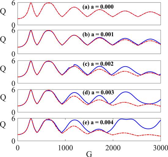
Figure 3. The dependence of response amplitude Q on HF signal amplitude G for a PDM particle with fixed mass m0 = 1 with five values of nonlinear strength a = [0, 0.001, 0.002, 0.003, 0.004]. The continuous blue lines represent the response curves obtained from the numerically computed response amplitudes using equation ( |
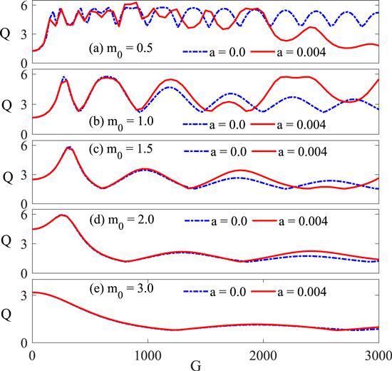
Figure 4. The dependence of response amplitude Q on HF signal amplitude G for a particle with constant mass (a = 0, shown with broken blue line) superimposed on the response curve of a particle with weak spatially varying mass (a = 0.004, shown with continuous red line) for five different values of the fixed rest mass m0: (a) m0 = 0.5, (b) m0 = 1.0, (c) m0 = 1.5, (d) m0 = 2.0 and (e) m0 = 3.0. Other system parameters are set as Ω = 13, ω = 0.65, γ0 = 0.27, λ = 0.9, φ = 0.1, V0 = k = 1, f = 0.05. |
According to Usama et al [45], constant mass influences VR initiated by the external periodic signal. Two distinct regimes of influence were identified, and a critical mass bordering both regimes, above which no enhancement of observed resonance due to HF signal modulation can be achieved by increasing the system's mass. The critical mass, herewith referred to as a cutoff or threshold mass was determined to be mthr = 2.375. Although our result in figure 4 corroborates this, we provide additional useful information that was not reported, particularly on the role of spatial mass variation. By comparing the features of figures 4(a)–(e), we can make the following deductions: (1) the number of resonance peaks reduces with increasing value of m0—implying that the magnitude of the multiresonance signature can be controlled by the rest mass; (2) as the value of the rest mass m0 increases from m0 = 0.5 to m0 = 3.0, the response amplitude Q(G=0) before the HF signal is activated approaches the global maximum response, Qmax. Therefore, there exists a value of the rest mass for which ${Q}_{(G=0)}={Q}_{\max }$, and it lies between 2 < m0 ≤ 3. The aforementioned features of figure 4 hold for both a = 0 and a = 0.004, however, only the former was reported in [45]. Consequently, the rest mass influences the features of VR in the same way for the two values of the nonlinear strength considered, and this we would later prove to hold for all weak spatially varying masses.
The effect of mass nonlinear strength a on the system's response can be further observed by comparing the resonance curves in figures 4 and 5 for the PDM system (12 ) with weak spatially varying mass (0 ≤ a ≤ 0.01), including the special case of constant mass (a = 0), and in figure 6 for particle with strong spatially varying mass 0.01 < a ≤ 0.1. Clearly, the multiresonance signatures observed at a = 0 for different rest masses m0 = 0.5, 1.0, 1.5, 2.0, 3.0 shown in panels (a)–(e) of figure 4 remains for a weak spatial mass variation a = 0.004. However, obvious changes in resonant behaviour emerged at high values of HF amplitude G, particularly at G ≥ 1000. This is highlighted in figure 4(c), where the last resonance peak is well pronounced at a = 0.004 compared to that of a = 0.0. Similar behaviour appears in figure 4(d) which has only three distinct resonance peaks. To project the effect of the nonlinear mass strength a on the observed behaviour in figure 4, especially on the possibility of controlling the system's response, we reproduced figure 4(b) for four values of the weak mass nonlinear strength a (0.001, 0.002, 0.003 and 0.004) superposed on the response curve for constant mass (a = 0.00) as presented in figure 5. Again, there the response behaviour of the system at low values of G (shown in figure 5(a) for G ∈ (0, 1500)) is insignificant. However, at large values of G in the regime G ∈ (2000, 2500) shown in figure 5(b), there is a significant difference in the resonance behaviour of the system for separate values of a as presented in figure 5(b). The observed difference accounts for the distinct feature at G ∈ (2500, 3000), which shows the peaks (maxima) at a = 0 and a = 0.001 coinciding with minima at a (= 0.002, 0.004).
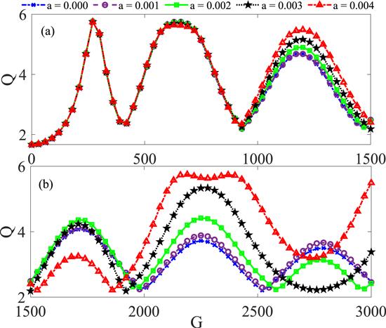
Figure 5. The variation of response amplitude Q on HF signal amplitude G; (a) G ∈ (0, 1500), (b) G ∈ (1500, 3000) for the PDM multistable system for four values of mass nonlinear strength a (=0.00, 0.001, 0.002, 0.003 and 0.004), when m0 = 1. Other parameters are set at Ω = 13, ω = 0.65, γ0 = 0.27, λ = 0.9, φ = 0.1, V0 = k = 1 and f = 0.05. |
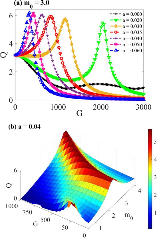
Figure 6. (a) Dependence of the response amplitude Q on HF amplitude G for a particle with strong spatially varying mass, (a = 0.030, 0.035, 0.040, 0.050 and 0.060) compared to the response curve (shown in figure 4(e)) for the system with constant mass a = 0.00 at m0 = 3. (b) Three-dimensional plot showing the dependence of the response amplitude Q on the amplitude of the HF signal G and the rest mass m0 at a = 0.04. Other parameters are set as : Ω = 13, ω = 0.65, γ0 = 0.27, λ = 0.5, φ = 0.1, V0 = k = 1 and f = 0.05. |
Remarkably, we found in figure 6 that at high values of mass nonlinear strength a, the VR exhibits significantly enhanced single peak reminiscent of single resonance, instead of multiple peaks characterizing multiresonance seen in figures 4 and 5 for low values of a. Figure 6(a) shows the dependence of response amplitude Q on the HF amplitude G for the PDM multistable system with strong mass variation (a = 0.02, a = 0.03, a = 0.035, a = 0.04, a = 0.05 and a = 0.012) superposed on the multiresonance curve of the system with constant mass (a = 0.00) at m0 = 3. This effect is not only a departure from the aforementioned second feature of the effect of rest mass on VR from figure 4, but also differs remarkably from what was reported for a system with constant mass, where the constant mass would not enhance VR when m > 2.375. Clearly, for a system with strong spatial variation, that is, a high value of the mass nonlinear strength, the rest mass significantly enhances resonance, particularly the global maximum as shown in figure 6(a) for m0 = 3 in contrast to the no-enhancement reported when the particle mass is either constant (a = 0) or has a weak spatial variation (a = 0.004) as shown in figure 4(e). Notice that while the maximum response amplitude Qmax increases with increasing nonlinear strength a, the response amplitude preceding the onset of VR remains constant, which signifies the enhancement capability of the nonlinear strength, the value of HF amplitude G at which resonance occur reduces. In addition, the single peak response curves showed that strong spatial variation leads the system from multiresonance to single resonance. We showed in figure 6(b) that the observed single resonance for the PDM particle with strong spatial variation traverses the rest mass. Figure 6(b) is a typical three-dimensional surface plot of the dependence of response amplitude Q on both the HF amplitude G and rest mass m0 for a particle with strong spatial variation in the range (G, m0) ∈ [(0, 1000), (0.2, 4)], with mass nonlinear strength a = 0.04. The single resonance appears as a band of single-peak resonances traversing the rest mass, forming a ridge-shaped elevation with the peak in red (see the colour bar) sandwiched by blue plains indicative of regimes with no enhancement. This implies that the single resonance observed at a high value of nonlinear strength is consistent at all values of rest mass.
As earlier mentioned, constant mass imposes two distinct regimes of influence on VR when the HF signal is switched on. The constant mass enhances observed VR below a threshold value, and above which no enhancement can be expected [45]. One may ask, how does the spatial variation in mass impact on the regimes in which the fixed rest mass influences the occurrence of VR? This question is crucial given the observed VR pattern shown in figure 6, where the fixed rest mass influenced resonance above the reported critical mass when the PDM particle has strong spatial variation. To answer the question, we characterized the system's response to variation in the fixed rest mass m0 when VR is initiated through the events around the threshold rest mass ${m}_{{0}_{{thr}}}$ in the two distinct classes of PDM multistable system, that is, particles with weak spatial variation (0 < a ≤ 0.01) and particles with strong spatial variation (0.01 < a ≤ 0.1). We compute the quantifier ${Q}_{\max }^{* }$ to establish the possibility of enhancing observed VR through the fixed rest mass in both cases. The ${Q}_{\max }^{* }$ is the ratio of the global maximum response amplitude Qmax to the onset response amplitude Q(G=0) before the HF signal becomes active, that is,42 ) on the rest mass m0 for (a) particles with weak spatial variation described by a = (0, 0.002, 0.004, 0.006, 0.008, 0.01) shown in figure 7(a), and (b) particles with strong spatial variation by a = (0.02, 0.03, 0.035, 0.04, 0.05, 0.06) shown in figure 7(b). Although the fixed rest mass m0 could enhance VR, and the mass nonlinear strength a influences the long-term dynamics of the system at all values of m0, figure 7(a) shows that VR can be enhanced or suppressed through the fixed rest mass independent of the value of the nonlinear strength for a PDM system with weak spatial variation. The existence of the threshold rest mass ${m}_{{0}_{{thr}}}$, above which the rest mass produces no enhancement is valid for weak spatial variation, and its value holds for all admissible values of a. In particular, the threshold rest mass which corresponds to ${m}_{{0}_{{thr}}}=2.4$ as highlighted by the vertical line cutting across figure 7(a) is in good agreement with the value of 2.375 reported in [45] for a particle with constant mass. The vertical line indicative of ${m}_{{0}_{{thr}}}$ partitions the figure into the two regimes, the region of influence on the left and the region of no influence (when ${Q}_{\max }^{* }=1$) to the right. Therefore, the results of Usama et al holds for a PDM particle with weak spatial mass variation. However, when the particle mass has strong spatial variation, the nonlinear strength does not only control the influence of the fixed mass on VR but dictates the dynamics when the threshold mass is exceeded. Specifically, figure 7(b) shows that the threshold rest mass ${m}_{{0}_{{thr}}}$ denotes the mass beyond which the reverse influence of the rest mass on VR is triggered. The observed VR is suppressed by increasing the value of the rest mass until a point where such increment yields no impact. However, a further variation of the rest mass beyond the threshold mass value triggers an enhancement. This accounts for the achievement of enhanced response in a particle with strong spatial variation beyond the critical mass as shown in figure 6(a) for ${m}_{0}=3(\gt {m}_{{0}_{{thr}}})$. Succinctly put, the impact of the fixed rest mass on VR of a particle with strong spatially varying mass can be classified into three distinct regimes: (1) region of influence marked by suppression relative to rest mass increase, (2) region of no influence whose magnitude is dependent on mass nonlinear strength a, and (3) region of reverse influence marked by enhancement relative to rest mass increase when the rest mass exceeds the threshold rest mass ${m}_{{0}_{{thr}}}$.
$\begin{eqnarray}{Q}_{\max }^{* }=\displaystyle \frac{{Q}_{\max }}{{Q}_{(G=0)}}.\end{eqnarray}$
${Q}_{\max }^{* }=1$ implies no VR enhancement by the system's rest mass. Figure 7 shows the dependence of ${Q}_{\max }^{* }$ computed from equation (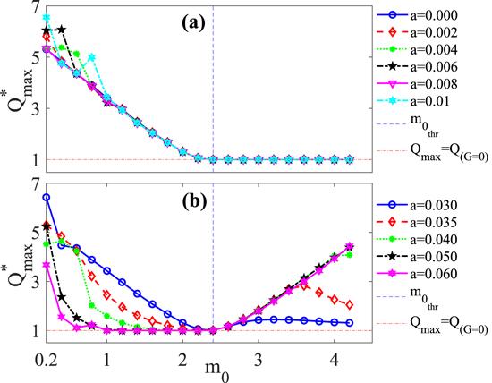
Figure 7. The dependence of ${Q}_{\max }^{* }$ computed from equation ( |
From the foregoing, we deduced that the mass nonlinear strength controls the resonance features of a PDM multistable system. For a particle with weak mass variation, the variation of the nonlinear strength altered the resonance signature, whereas the overall influence of rest mass on VR is unaltered. Below a threshold rest mass ${m}_{{0}_{{thr}}}$, the fixed rest mass enhanced (or suppressed) VR when the nonlinear strength is weak. However, when the mass variation is strong, the nonlinear strength dictated responses, and significantly altered the system (equation (12 )) dynamics by driving the resonance behaviour from multiresonance to single resonance. Furthermore, the nonlinear strength controlled the influence of the rest mass on VR, such that a reverse influence is triggered at the threshold mass rest. In general, the parameters of the variable mass distribution complemented the HF signal which governed the observed VR in the PDM multistable system.
5.2. Inducing VR from PDM parameters
Herein, we employed the cooperation of the HF signal and the PDM parameters to produce VR at the low frequency ω by varying the PDM parameters (m0, a) in the presence of the HF signal parameters (G, Ω). We achieved single resonance as shown in figure 8(a) for the dependence of the response amplitude Q on the rest mass m0 at a = 0.005, G = 250, and in figure 8(b) for the dependence of Q on nonlinear strength a at m0 = 3, G = 50 for four different values of the HF Ω (= 13, 18, 23, 30). In both instances, single peak PDM-induced resonance which is mostly encountered in an archetypical monostable system was obtained. The maximum response of the mass nonlinear strength-induced resonances occur at extremely high values of the mass nonlinear strength. Varying the high frequency Ω increases the maximum response Qmax of the rest mass-induced single resonance, and the value of mass nonlinear strength at which resonance occur aVR in the mass nonlinear strength-induced resonance as depicted in figures 8(a) and (b), respectively. In addition, the HF amplitude G could also control the PDM-induced resonance, which is strongly susceptible to HF amplitude modulation. To investigate the effect of the HF amplitude G on the rest mass-induced single resonance presented in figure 8(a), we plotted the response curve at Ω = 13, a = 0.004 for different values of G in figure 9(a)–(d). The HF amplitude G controls the response curve and leads it from single resonance into bi-resonance as shown in 9(a) for G = (50, 100, 150, 200). Bi-resonance is observed for other values of G (= 250, 450, 600, 750) as shown in figures 9(b)–(c), and the phenomenon becomes multiresonance at higher values of G (= 900, 1200) as shown in figure 9(d). Moreover, the increase in the HF amplitude of the mass nonlinear strength induced resonance in figure 8(b) at Ω = 13, m0 = 3 leads the system from single resonance (presented in figure 10(a) for G = 50, 100, 150) to bi-resonances (presented in figure 10(b)–(a) for G = 50, 100, 150). Hence, figures 9 and 10 prove that varying G impacts on the PDM-induced resonant states of the system and contribute meaningfully towards leading the system to parameter regimes that could yield different resonance states.
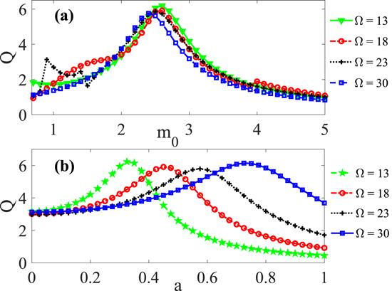
Figure 8. (a) The variation of response amplitude Q on (a) fixed rest mass m0 at a = 0.005, G = 250, (b) mass nonlinear strength a at m0 = 3, G = 50, for four values of HF Ω (= 13, 18, 23, and 30). Other parameters are set at ω = 0.65, γ0 = 0.27, λ = 0.9, φ = 0.1, V0 = k = 1 and f = 0.05. |
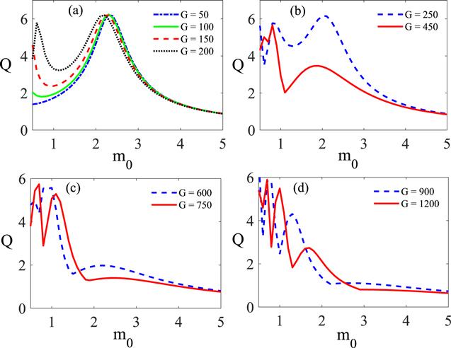
Figure 9. The variation of the response amplitude Q on a rest mass m0 for four lower values of the amplitude of the high-frequency driving force G (= 50, 100, 150 and 200); (b) G = 250 and 450; (c) G = 600 and 750; (d) for higher values of the amplitude, G = 900 and 1200. Other parameters are set as: Ω = 13, ω = 0.65, a = 0.004, γ0 = 0.27, λ = 0.5, φ = 0.1, V0 = k = 1 and f = 0.05, = 0.004. |

Figure 10. Variation of the response amplitude Q with the nonlinear strength a for different values of the amplitude of the HF G: (a) G = 50, G = 100, G = 150, (b) G = 200 , (c) G = 250, (d) G = 450. While other parameters are set as m0 = 3, Ω = 13, ω = 0.65, γ0 = 0.27, λ = 0.9, φ = 0.1, V0 = 1, k = 1, f = 0.05. |
Next, we considered the effect of nonlinear strength on the PDM-induced resonance in the presence of the bi-harmonic driving signal. First, we showed that the observed rest mass-induced bi-resonance in a particle with weak spatial variation with mass nonlinear strength a = 0.004 presented in figure 9(c) for G = 750 is replicated at another low value of the nonlinear strength, specifically at a = 0.01 as shown in figure 11(a). However, the response amplitude Q as a function of the fixed rest mass m0 presented in figure 11(b)–(d) for high values of a (=0.02, 0.03, 0.04) shows the PDM multistable system exhibited single peak rest mass-induced resonance. When a = 0.04, single and bi-resonance could be produced depending on the choice of HF amplitude G as seen in the three-dimension surface plot of (Q, G, m0) (see figure 6). Furthermore, both the maximum response amplitude Qmax and the rest mass at which resonance occurs, ${m}_{{0}_{{VR}}}$ increase with increasing a. This implies that the features of the m0-induced resonance can be effectively controlled by the nonlinear strength.

Figure 11. The variation of the response amplitude Q on a rest mass m0 (a) for a = 0.01; (b) a = 0.02; (c) a = 0.03; (d) a = 0.04. Other parameters are fixed at G = 750, Ω = 13, ω = 0.65, γ0 = 0.27, λ = 0.5, φ = 0.1, V0 = k = 1 and f = 0.05. |
Furthermore, we examined the influence of fixed rest mass on the features of the mass nonlinear strength-induced single resonance presented in for G = 50 in figure 10(a). Figure 12(a) shows the dependence of the response amplitude Q on the mass nonlinear strength a for six values of the rest mass m0 (= 0.5, 1.0, 1.5, 2.0, 2.5 and 3.0) with fixed values of the HF signal parameters (G = 50, Ω = 13). The system's response exhibits single resonance when m0 = 3. However, small values of the rest mass significantly suppress the response (see the response curve for m0 = 2.5). With a further decrease in value of the fixed rest mass (through m0 = 2.0 to m0 = 0.5), the maximum response amplitude Qmax approaches a limiting value where it coincides with the outset response Q(G=0), and consequently, the rest mass no longer impacts on the resonance features, suggesting a threshold rest mass. Surely, the influence of the fixed rest mass on the observed PDM-induced resonance (Q versus a) contrasted with its effect on traditional VR (Q versus G) highlighted in section 5.1 . The rest mass's influence on traditional VR diminishes with a mass increase until it reaches a threshold mass, beyond which further suppression seizes, or reverse influence is initiated in a particle with strong mass variation (see figure 7). Thus, figure 12(a) suggests the existence of a threshold rest mass above which amplified responses can be achieved in the PDM-induced resonance.

Figure 12. (a) Dependence of the response amplitude Q on the nonlinear strength a for different values of the rest mass m0 (m0 = 0.5, m0 = 1.0, m0 = 1.5, m0 = 2.0, m0 = 2.5 and m0 = 3.0). (b) The dependence of ${Q}_{\max }^{* }$ computed from equation ( |
To obtain the threshold rest mass ${m}_{{0}_{{thr}}}$, we redefine ${Q}_{\max }^{* }$ as the ratio of the maximum response amplitude Qmax to the outset response amplitude Q(a=0), that is, the response amplitude for the particle with constant mass. Thus:43 )) on the fixed rest mass m0 is presented in figure 12(b) for four values of HF amplitudes (G = 10, 25, 50, 100). The figure 12(b) shows a gradual increase of the fixed rest mass would produce no enhancement of the nonlinear strength-induced resonance until the fixed rest mass equals or exceeds a threshold, ${m}_{{0}_{{thr}}}=2.325$ for the four values of G, which is consistent with our observation in figure 12(a). The nature of the influence of HF amplitude G on the PDM-induced resonance is presented through a three-dimensional plot of m0 versus a versus Q for HF amplitudes G = 10, G = 25, G = 50 and G = 100 in figures 13(a)–(d), respectively. Figure 13 reproduced the well-enhanced single peak resonance, the emergence of double resonance and other notable features arising from HF modulation presented in figures 8–12. Increasing G does not only create new m0-induced resonances but constrains the peaks towards lower values of a as can be seen in figures 13(c)–(d). The transition from single resonance to double resonance at higher values of G becomes more prominent with increasing nonlinear strength a. The emergence of new peaks at extremely large values of a can be seen in figure 13(d).
$\begin{eqnarray}{Q}_{\max }^{* }=\displaystyle \frac{{Q}_{\max }}{{Q}_{(a=0)}}.\end{eqnarray}$
${Q}_{\max }^{* }=1$ indicates Qmax coincides with the outset response Q(a=0), which implies no enhancement of PDM-induced resonance is achieved at a particular rest mass. The variation of ${Q}_{\max }^{* }$ (computed from equation (
Figure 13. Three-dimensional plot showing the dependence of the response amplitude Q on the rest mass m0 and the nonlinear strength a of the mass function, for four distinct values of the amplitude of the fast signal G: (G = 10, 25, 50 and 100), presented in (a)–(d) respectively. Other parameters of the system are set at : Ω = 13, ω = 0.65, γ0 = 0.27, λ = 0.5, φ = 0.1, V0 = k = 1 and f = 0.05. |
In the preceding discussions, we showed that single and double resonance states can appear through the PDM parameters from an otherwise multiresonance state in a multistable system with a variable mass system. In general, the system's response to the variation of either the HF signal parameters or the rest mass is influenced by the strength of spatial mass nonlinearity. The qualitative features of the influence of the mass nonlinear strength in driving the system from a single resonance state to double resonance condition with high nonlinear strength and bi-harmonic forcing were also revealed. The possibility of generating resonant states other than multiresonance through the variable mass parameters is attributable to the potential deformation characteristics of the variable mass as shown in (6 ). Essentially, when particle mass varies with position, the system potential (6 ) is modified (as (14 )), consequently its response to parameter modulation alters significantly. Vincent et al [40] showed clear evidence of deformation-induced double resonances in a particle evolving in a nonlinear asymmetrical Remoissenet–Peyrard type deformable potential substrate. Ultimately, the role of the variable mass parameters is similar to that of potential deformation, as well as contributions from perturbation of damping and external forcing. This is established by considering the influence of the PDM nonlinear strength on the potential deformation, particularly on the depth of well as defined by equation (17 ). We re-produced the PDM nonlinear strength-induced resonance curve shown in figures 8(b) and 10(a) for m0 = 3, Ω = 13, G = 50 as resonance curves for the dependence of response amplitude Q on the potential well depth, d as presented in figure 14. The depth, d is computed over the range of nonlinear strength a ε [0, 1] for four integer values n = ±1, ±3, ±5 and ±7. The Q versus a curves in figures 8(b) and 10(a) are expectedly similarly to the Q versus d curves in figure 14 since the nonlinear strength a and potential well depth d are linearly related (equation (17 )) at small integer values of n as shown in figure 14. Thus, the PDM-induced resonance is associated with the variation in well depth as the PDM parameters are varied.

Figure 14. Variation of the response amplitude, Q with the depth of the potential well, d for three values of the number of well n( ±3, ±5, ±7). The inset shows the dependence of response amplitude Q on the depth of the well for n = ±1. The response curves correspond to the PDM nonlinear strength a-induced curve for m0 = 3 shown in figure 8(b) for Ω = 13, and figure 10(a) for G = 50. The potential well depth d is computed from equation ( |
6. Conclusion
In this paper, we presented the results of our numerical investigation of vibrational resonance in a PDM multistable system describing the motion of a particle with a periodic potential, subjected to both bi-harmonic excitation and position-dependent nonlinear dissipative damping. Our results extended and generalized previous studies on VR in a multistable system with asymmetric potential with unitary mass and constant mass by Roy-Layinde et al [39] and Usama et al [45], respectively. For the PDM particle considered, the traditional HF-induced VR produced multiresonance at low values of the mass nonlinear strength a(0 ≤ a ≤ 0.01) , and single or double resonance at high values of the mass nonlinear strength a(0.01 < a ≤ 1). In both cases, the rest mass m0 influenced the observed resonances, and we identified a threshold mass of ${m}_{{0}_{{thr}}}=2.4$ beyond which no enhancement or suppression could be achieved through the rest mass for a particle with weak spatial variation, and beyond which further modulation produced reverse influence for a particle with strong spatial mass variation. Furthermore, we showed that modulation of the PDM parameters induced unconventional single and double resonances which could be controlled by the HF signal parameters (G, Ω). The HF amplitude G led the PDM-induced resonances from single resonance into double resonances. The system's response to modulation of the nonlinear strength a in the presence of HF signal was enhanced when the rest mass either equal or exceeded the threshold mass ${m}_{{0}_{{thr}}}=2.325$. Therefore, besides controlling the HF signal-induced VR, the variable mass parameters initiated and controlled the resonant conditions of the PDM multistable system. We conclude that the resonance phenomena observed in a one-dimensional PDM multistable system modelling a particle with variable mass described by a regular mass function (of the form (9 )) are not only influenced by nonlinear dissipation, frictional inhomogeneity, initial phase shift and constant mass [39, 45], but the mass nonlinear strength governing spatial mass variation. In fact, variable mass cooperates with the HF signal to determine the nature and structure, and control observed resonance. Lastly, we found that the strength of spatial mass variation and HF amplitude determined the spheres of influence of particle mass on the observed traditional VR and unconventional PDM-induced resonance, respectively.
The use of system parameters such as external signal, noise and time delay in controlling nonlinear phenomena such as multistability, synchronization and resonance is well established. Recently, it was suggested that the nature of the variable mass distribution could determine the outcome of a system's response to dual-frequency driving forces as the nonlinearity strength of the mass leads a system modelling vibration inversion mode of NH3 from single resonance to double resonance [48]. Also, while the possibility of inducing resonances from variable mass parameters was first reported in the literature by Roy-Layinde et al [49], the possibility of generating single resonance from variable mass parameters in a multistable system is novel. We emphasize that the control of the resonant behaviour of a multistable system by PDM parameters to yield different resonant states is advantageous based on the significance of multistability control in applied nonlinear science. For instance, multistability can create inconvenience in the design of commercial devices with certain specifications where multistability is undesirable or the need to stabilize the system in a preferred state against a noisy environment. This way a single or double resonant state would serve better [19]. On the contrary, the coexistence of different stable states associated with multistability 5 offers great possibilities in inducing flexible system performance by leveraging the right control strategies to initiate a definite switching between different resonant states without necessarily choosing a new parameter regime as would be expected if the system undergoes single resonance. VR is a useful tool for the achievement of higher laser modulation bandwidths which is desirable in applications like multigigabit optical fibre transmitters [25, 48, 49]. Moreover, VR could be suitable for designing measurement techniques, and thus, exploring HF parametric vibrations can find practical applications in communications systems as well as in the detection and assessment of structural damage in systems with breathing cracks, thus, suggesting new directions for VR investigations, and in which the need for the consideration of variable particle mass appears crucial.