


1. Introduction
The O(N) spin model [1], also referred to as the O(N) nonlinear σ model in field-theoretic parlance, is central to the study of critical phenomena. It has been subjected to extensive studies over several decades via both field-theoretical approaches and statistical mechanical methods. Within the comprehensive family of O(N) spin models, the models for N = 1, 2, and 3 are of particularly significant interest as they correspond directly to the Ising, XY, and Heisenberg models, respectively.
To surpass the constraints of perturbation theory, the powerful numerical tool the Monte Carlo (MC) method [2] is widely used to simulate the O(N) spin model. However, the Metropolis scheme, which is frequently employed [3], undergoes significant ‘critical slowing down', consequently impairing computational efficiency near the critical point [4]. Addressing this issue, various non-local update algorithms have been put forward, encompassing multigrid techniques and cluster update algorithms [5]. Among these, the cluster update algorithms prove to be the most effective for the O(N) spin model [6]. On the flip side, for local update algorithms, the worm technique emerges as a promising contender. This algorithm, extensively deployed in both classical and quantum systems [7, 8], exhibits superior efficiency at criticality, typically applied to graphical representations complying with Kirchhoff-like conservation laws. Fundamentally, a worm algorithm modifies configuration graphs by introducing two defects that infringe these conservation laws, moves them around according to the balance condition for MC simulations, and ultimately removes them once they reconvene. Hence, to develop worm-type algorithms for particular models, like the O(N) spin model, it is often required to first formulate their graphical representations.
Graphical representations for the Ising (N = 1) and XY (N = 2) models are well established. For the Ising model, a specific graphical representation introduces a non-negative integer variable on each lattice bond, visually represented by the number of lines drawn on the corresponding bond (figure 1(a)). A configuration makes a non-zero contribution only when it satisfies the Eulerian condition, which requires each site to be connected by an even number of lines. On the other hand, a prevalent graphical representation for the XY model assigns two types of non-negative variables to each bond, symbolizing currents flowing in positive and negative directions, respectively. These currents, in their entirety, satisfy conservation at each site, reflecting the Kirchhoff flow-conservation law (figure 2(a)). For the sake of convenience, configurations in these two representations are referred to as the Ising subgraphs and the XY subgraphs in this paper, respectively.
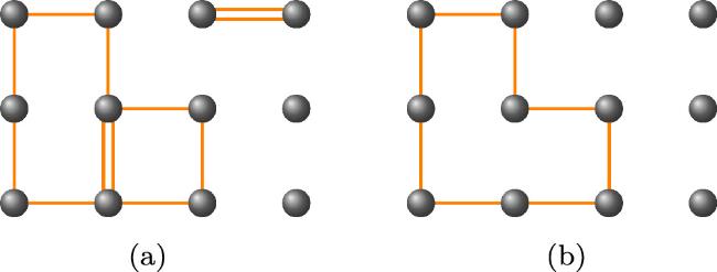
Figure 1. Typical graphical configurations for the Ising model in representation ( |
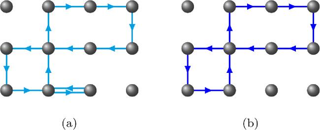
Figure 2. Typical graphical configurations for the 2D XY model in representation ( |
When considering an arbitrary value of N > 2, studies on graphical representations have also made significant advances in the past decade. In 2010, Wolff put forward a graphical representation defined by a single set of bond variables, depicted by lines on the corresponding bonds [9]. Each site incorporates a type of switch-board, creating pairwise connections among all neighboring lines. This approach implies that a range of configurations can be attributed to one specific set of bond variables, necessitating the inclusion of symmetry factors. A few years later, two distinct representations each depicted by N sets of bond variables were proposed. These representations view configurations as the combination of multiple subgraph copies [10, 11]. Specifically, a configuration in [10] is the union of one XY graph copy and N − 2 Ising graph copies. Conversely, a configuration in [11] is the combination of N Ising graph copies.
In this work, we devise a systematic series of graphical representations for the O(N) spin model using a streamlined approach. This series is parameterized by an integer ℓ (0 ≤ ℓ ≤ N/2). To establish these representations, we dissect the total spin vector into a weighted sum of ℓ copies of XY vectors and N − 2ℓ copies of Ising vectors. By incorporating currents (flows) for the XY vectors and undirected bonds for the Ising vectors, we obtain the graphical representation after integrating out the spin degree of freedom. The resulting configuration consists of ℓ copies of XY subgraphs and N − 2ℓ copies of Ising subgraphs. Notably, when ℓ = 0 and 1, our representations reduce to those proposed in [10, 11]. Further, by introducing two defects in these graphical representations, we develop corresponding worm algorithms for any arbitrary N and potential ℓ. Using these algorithms, we conduct large-scale simulations on a simple-cubic lattice with a linear size of up to L = 96 for N = 2, 3, 4, 5, and 6, across all possible ℓ values. We deduce and compare the dynamic exponents for each variant of the worm algorithms from the fitting of the integrated autocorrelation time for an ‘energy-like' observable. Our simulation results reveal that the algorithm efficiency increases with the number of XY subgraph copies in a single configuration, i.e. a larger ℓ promotes higher efficiency. In the best cases, dynamic exponents can reach z = 0.20(1), 0.32(2), 0.22(1), 0.26(3), and 0.16(2) for N = 2, 3, 4, 5, and 6, respectively. Consequently, the efficiency of worm-type algorithms is comparable with that of cluster update methods [12], significantly outperforming the Metropolis algorithm which has a dynamic exponent z ≈ 2.
In addition to MC simulations, researchers are exploring other advanced numerical methods for applications on the O(N) spin model, among which the tensor network renormalization (TNR) [13] is one of the most promising. It starts by representing the partition function or the ground state wavefunction as a tensor network state that is formed by taking the product of local tensors defined on the lattice sites. However, applying this method to the O(N) spin model is challenging because each spin has infinite degrees of freedom, and the conventional method of constructing the local tensors fails. For N = 1 and 2, researchers proposed a novel scheme to construct the tensor representation using character expansions [14]. These representations can actually be derived by slightly reformulating the conventional bond-based graphical representations for the Ising and XY models. Therefore, we expect that the development of graphical representations would provide a convenient foundation for investigating the O(N) spin model with TNR and other numerical methods.
This paper is structured as follows: in section 2 , we provide a succinct introduction to the Hamiltonian and the partition function for the O(N) spin model, and then revisit the graphical representations for the Ising and XY models before deriving the family of graphical representations for the O(N) spin model. The worm algorithms are introduced in section 3 , followed by the presentation of our simulation results in section 4 . We conclude the paper with a discussion in section 5 .
2. Hamiltonian and graphical representations
The O(N) spin model characterizes N-component spin vectors with inner-product interactions on a lattice, as represented by the Hamiltonian:
$\begin{eqnarray}{ \mathcal H }/{k}_{{\rm{B}}}T=-\displaystyle \sum _{\langle i,j\rangle }K{{\boldsymbol{S}}}_{i}\cdot {{\boldsymbol{S}}}_{j},\end{eqnarray}$
where Si is the N-dimensional unit spin vector on site i, explicitly expressed as ${\boldsymbol{S}}={\sum }_{\mu =1}^{N}{S}_{\mu }{{\boldsymbol{e}}}_{\mu }$ with eμ the unit vector along the μ direction, subject to the constraint ${\sum }_{\mu =1}^{N}{S}_{\mu }^{2}=1$. The symbol K > 0 denotes the ferromagnetic coupling strength for each nearest neighbor pair, kB is the Boltzmann factor and T represents the system's temperature. The symbol ⟨i, j⟩ indicates that the summation covers all nearest neighboring sites. The corresponding partition function is given by: $\begin{eqnarray}{ \mathcal Z }=\left(\displaystyle \prod _{i}\int { \mathcal D }{{\boldsymbol{S}}}_{i}\right)\displaystyle \prod _{\langle i,j\rangle }{{\rm{e}}}^{K{{\boldsymbol{S}}}_{i}\cdot {{\boldsymbol{S}}}_{j}}.\end{eqnarray}$
Here, the integral $\int { \mathcal D }{\boldsymbol{S}}$ signifies the uniform measure of the vector S, defined as $\int { \mathcal D }{\boldsymbol{S}}={\int }_{| {\boldsymbol{S}}| =1}{{\rm{d}}}^{N}{\boldsymbol{S}}$, with N denoting the dimension of the vector. Notice that, to maintain the elegance of partition function expressions, we always omit trivial factors, that poses no physical implications.In the following parts, we begin by providing a brief overview of the well-established graphical representations for the Ising (N = 1) and XY (N = 2) models. Using these as a basis, we then construct a series of graphical representations adaptable to any given value of N. Note that, for the sake of simplicity, our illustrations in this section are confined to the square lattice. However, our derivation is applicable to any type of lattice in any spatial dimension.
2.1. N = 1: the Ising model
The Ising model characterizes unit spin vectors on the lattice that can either point upwards or downwards. Consequently, its partition function is given by4 ), each with a different number of lines on each bond. The latter factor in each summation term implies that only when nij fulfills the constraint at any site i:
$\begin{eqnarray}{{ \mathcal Z }}_{\mathrm{Is}}=\displaystyle \sum _{\{{s}_{i}\}}\displaystyle \prod _{\langle i,j\rangle }{{\rm{e}}}^{{{Ks}}_{i}{s}_{j}},\end{eqnarray}$
where si = ±1 signifies the spin vector at site i. The notation {·} suggests that the index inside the brackets iterates over all possible values. By employing a Taylor-series expansion to the Boltzmann statistical factor, we obtain $\exp ({{Ks}}_{i}{s}_{j})\,={\sum }_{{n}_{{ij}}=0}^{+\infty }{K}^{{n}_{{ij}}}{\left({s}_{i}{s}_{j}\right)}^{{n}_{{ij}}}/{n}_{{ij}}$, where nij = 0, 1, 2, … is the variable defined on each bond. This expansion gives us a new form for the partition function: $\begin{eqnarray}{{ \mathcal Z }}_{\mathrm{Is}}=\displaystyle \sum _{\{{n}_{{ij}}\}}\left(\displaystyle \prod _{\langle i,j\rangle }\displaystyle \frac{{K}^{{n}_{{ij}}}}{{n}_{{ij}}!}\right)\left(\displaystyle \prod _{i}\displaystyle \sum _{{s}_{i}=\pm 1}{s}_{i}^{\displaystyle \sum _{j\in {\mathbb{E}}(i)}{n}_{{ij}}}\right),\end{eqnarray}$
where ${\mathbb{E}}(i)$ signifies the set of nearest neighboring sites of site i. As depicted in figure 1(a), if we draw a number of undirected lines on each bond equivalent to the corresponding bond variable nij, we get a graph for every summation term in the partition function equation ( $\begin{eqnarray}{{ \mathcal L }}_{i}\equiv \mathrm{mod}\left(\displaystyle \sum _{j\in {\mathbb{E}}(i)}{n}_{{ij}},\,2\right)=0,\end{eqnarray}$
will the entire summation term make a non-zero contribution. This requirement implies that the degree of each site in the graph should be even, or alternatively, the graph can be seen as composed of closed loops. These non-zero contribution graphs are termed valid configurations, and if we use GIs to denote all of them, the partition function can be written in a graphical form: $\begin{eqnarray}{{ \mathcal Z }}_{\mathrm{Is}}=\displaystyle \sum _{{G}_{\mathrm{Is}}}\displaystyle \prod _{\langle i,j\rangle }{W}_{\mathrm{Is}}({n}_{{ij}}),\end{eqnarray}$
where WIs(n) ≡ Kn/n! stands for the weight factor contributed by each bond.Consequently, we construct a graphical representation for the Ising model, in which configurations are composed of closed-loop graphs founded on the bond framework. In this configuration graph, each bond imparts a weight factor WIs(n), dictated by the number of lines, n, present on it.
The above graphical representation differs from the commonly employed one for the Ising model, as depicted in figure 1(b). In the conventional representation, the constraint of even degree at each site still applies, but the bond variables nij can only adopt two values: 0 or 1. In graphical terms, loops in the graph should not share any bonds or traverse a bond more than once. This results in the following expansion for the partition function:6 ) that maintain the same parity of line numbers on each bond. Alternatively, if we shift our focus from the bonds to the sites, we can express the partition function of the Ising model in a tensor form as follows:
$\begin{eqnarray}{{ \mathcal Z }}_{\mathrm{Is}}=\displaystyle \sum _{{\widetilde{G}}_{\mathrm{Is}}}\displaystyle \prod _{\langle i,j\rangle }{\widetilde{W}}_{\mathrm{Is}}({n}_{{ij}}),\end{eqnarray}$
Here, ${\widetilde{G}}_{\mathrm{Is}}$ represents all graphs conforming to the above criteria, and ${\widetilde{W}}_{\mathrm{Is}}(n)\equiv {\tanh }^{n}K$ is the associated weight factor for each bond. Indeed, we can derive this representation by summing over all graphs in representation ( $\begin{eqnarray}{{ \mathcal Z }}_{\mathrm{Is}}=\displaystyle \sum _{\{{n}_{{ij}}\}}\displaystyle \prod _{i}{{{\mathbb{T}}}_{\mathrm{Is}}}^{(i)},\end{eqnarray}$
where ${{{\mathbb{T}}}_{\mathrm{Is}}}^{(i)}$ is a tensor on site i, given by ${{{\mathbb{T}}}_{\mathrm{Is}}}^{(i)}={\prod }_{j\in {\mathbb{E}}(i)}\sqrt{{\widetilde{W}}_{\mathrm{Is}}({n}_{{ij}})}\delta (\mathrm{mod}({\sum }_{j\in {\mathbb{E}}(i)}{n}_{{ij}},2))$. Notably, this tensor representation is consistent with that proposed in [14] for the Ising model.2.2. N = 2: the XY model
The XY model characterizes unit planar vectors at each lattice site, with the partition function expressed as:
$\begin{eqnarray}{{ \mathcal Z }}_{{xy}}=\left(\displaystyle \prod _{i}\int {\rm{d}}{\phi }_{i}\right)\displaystyle \prod _{\langle i,j\rangle }{{\rm{e}}}^{K\cos ({\phi }_{i}-{\phi }_{j})},\end{eqnarray}$
where we have redefined the spin vector on site i in terms of its angle φi ∈ [0, 2π) with respect to a predetermined direction. By splitting the cosine function into half of the sum of ${{\rm{e}}}^{{\rm{i}}({\phi }_{i}-{\phi }_{j})}$ and ${{\rm{e}}}^{-{\rm{i}}({\phi }_{i}-{\phi }_{j})}$ and subsequently expanding these exponential functions into their respective Taylor series [7], we achieve: $\begin{eqnarray}{{\rm{e}}}^{K\cos ({\phi }_{i}-{\phi }_{j})}=\displaystyle \sum _{{m}_{{ij}}^{\pm }=0}^{+\infty }\displaystyle \frac{{\left(\tfrac{K}{2}\right)}^{{m}_{{ij}}^{+}+{m}_{{ij}}^{-}}}{{m}_{{ij}}^{+}!\,{m}_{{ij}}^{-}!}{{\rm{e}}}^{{\rm{i}}({m}_{{ij}}^{+}-{m}_{{ij}}^{-})({\phi }_{i}-{\phi }_{j})}.\end{eqnarray}$
After integrating over all the angle variables φi, we can represent the partition function as: $\begin{eqnarray}{{ \mathcal Z }}_{{xy}}=\displaystyle \sum _{\{{m}_{{ij}}^{\pm }\}}\left(\displaystyle \prod _{\langle i,j\rangle }\displaystyle \frac{{\left(\tfrac{K}{2}\right)}^{{m}_{{ij}}^{+}+{m}_{{ij}}^{-}}}{{m}_{{ij}}^{+}!\,{m}_{{ij}}^{-}!}\right)\displaystyle \prod _{i}\delta ({{ \mathcal F }}_{i}),\end{eqnarray}$
with $\begin{eqnarray*}{{ \mathcal F }}_{i}=\displaystyle \sum _{j\in {\mathbb{E}}(i)}\mathrm{sgn}(i\to j)({m}_{{ij}}^{+}-{m}_{{ij}}^{-}),\end{eqnarray*}$
where the integer bond variables ${m}_{{ij}}^{\pm }$ can take values of 0, 1, 2, …, and ${{ \mathcal F }}_{i}$ represents the overall out-flow of site i. The symbol $\mathrm{sgn}(i\to j)$ equals either +1 or −1 based on whether i → j is in line with or against the chosen positive direction for each direction (for example, we opt for the upward and rightward directions in a 2D square lattice, as demonstrated in figure 2). In contrast to the Ising model, we draw directed lines on each bond, as illustrated in figure 2(a). These lines are categorized into two types, based on whether their directions are positive or negative. We ensure that the numbers of both types are equal to ${m}_{{ij}}^{+}$ (positive) and ${m}_{{ij}}^{-}$ (negative), respectively. The Dirac δ functions in the partition function, which stem from the integration of φi's, indicate that for any site i, we have $\begin{eqnarray}{{ \mathcal F }}_{i}\equiv \displaystyle \sum _{j\in {\mathbb{E}}(i)}\mathrm{sgn}(i\to j)({m}_{{ij}}^{+}-{m}_{{ij}}^{-})=0.\end{eqnarray}$
This implies that the combination of positive- and negative-directed lines can be effectively treated as a conserved current (flow) defined on the bond structure. Consequently, we can represent valid configurations as graphs composed of directed closed loops. Furthermore, in these graphs, each bond can have multiple lines along both directions simultaneously. Let Gxy denote all such graphs, the partition function ${{ \mathcal Z }}_{{xy}}$ can then be expressed as: $\begin{eqnarray}{{ \mathcal Z }}_{{xy}}=\displaystyle \sum _{{G}_{{xy}}}\displaystyle \prod _{\langle i,j\rangle }{W}_{{xy}}({m}_{{ij}}^{\pm }),\end{eqnarray}$
where ${W}_{{xy}}({m}^{\pm })\equiv {\left(K/2\right)}^{{m}^{+}+{m}^{-}}/({m}^{+}!{m}^{-}!)$ is the bond weight factor. This leads to a graphical representation in which configurations are graphs made up of directed closed loops. Each bond can be traversed simultaneously from both directions, contributing a weight factor Wxy(m+, m−). The weight factor depends solely on the numbers of lines along the positive and negative directions, or m+ and m−, on the bond.Indeed, by applying the substitution ${m}_{{ij}}={m}_{{ij}}^{+}-{m}_{{ij}}^{-}$ and ${\bar{m}}_{{ij}}=\min \{{m}_{{ij}}^{+},{m}_{{ij}}^{-}\}$, and subsequently summing over all ${\bar{m}}_{{ij}}$ variables, we can transform the graphical representation into a more common form:
$\begin{eqnarray}{{ \mathcal Z }}_{{xy}}=\displaystyle \sum _{{\widetilde{G}}_{{xy}}}\displaystyle \prod _{\langle i,j\rangle }{\widetilde{W}}_{{xy}}({m}_{{ij}}),\end{eqnarray}$
where the bond variable mij is an integer taking values 0, ±1, ±2, …, the bond weight factor ${\widetilde{W}}_{{xy}}(m)$ is defined as Im(K), corresponding to the modified Bessel function of the first kind with order m, and ${\widetilde{G}}_{{xy}}$ denotes all graphs that also consist of directed closed loops. However, it imposes a constraint that a bond can only be traversed from a single direction at a time, implying that all lines on the same bond should follow the same direction: either positive or negative. In this representation, the quantity and direction of lines on a bond represent the absolute value and the sign of mij, respectively. A typical graphical configuration is illustrated in figure 2(b). Following a similar approach to the Ising model, we can apply a reformulation of the graphical representation in a tensor form as follows: $\begin{eqnarray}{{ \mathcal Z }}_{{xy}}=\displaystyle \sum _{\{{m}_{{ij}}^{\pm }\}}\displaystyle \prod _{i}{{{\mathbb{T}}}_{{xy}}}^{(i)},\end{eqnarray}$
where ${{{\mathbb{T}}}_{{xy}}}^{(i)}={\prod }_{j\in {\mathbb{E}}(i)}\sqrt{{\widetilde{W}}_{{xy}}({m}_{{ij}}^{\pm })}\delta (\mathrm{sgn}(i\to j)({m}_{{ij}}^{+}-{m}_{{ij}}^{-}))$ is a tensor defined on site i. This tensor representation is identical to the one introduced in [14] for the XY model.2.3. Arbitrary N
To obtain graphical representations for any integer N ≥ 1, we first analyze the structure of the N-dimensional spin vector S and discover that it can be decomposed into a sum of ℓ copies of two-dimensional (2D) and N − 2ℓ copies of one-dimensional (1D) orthogonal spin vectors, with 0 ≤ ℓ ≤ N/2. This can be expressed as:
$\begin{eqnarray}{\boldsymbol{S}}=\displaystyle \sum _{\alpha }{{ \mathcal A }}_{\alpha }{{\boldsymbol{S}}}^{(\alpha )}+\displaystyle \sum _{\beta }{{ \mathcal B }}_{\beta }{{\boldsymbol{s}}}^{(\beta )},\end{eqnarray}$
where ${{ \mathcal A }}_{\alpha }{{\boldsymbol{S}}}^{(\alpha )}={S}_{2\alpha -1}{{\boldsymbol{e}}}_{2\alpha -1}+{S}_{2\alpha }{{\boldsymbol{e}}}_{2\alpha }$ (α = 1, 2, …, ℓ) and ${{ \mathcal B }}_{\beta }{{\boldsymbol{s}}}^{(\beta )}={S}_{\beta +2{\ell }}{{\boldsymbol{e}}}_{\beta +2{\ell }}$ (β = 1, 2, …, N − 2ℓ) represent the decomposed 2D or 1D spin vectors. The non-negative coefficients ${{ \mathcal A }}_{\alpha }$ or ${{ \mathcal B }}_{\beta }$ indicate the magnitude, while the unit vectors S(α) in 2D or s(β) in 1D represent the orientations (∣S(α)∣ = 1 and ∣s(β)∣ = 1). Notably, the constraint for the spin vector's unitarity becomes a requirement for the coefficients: $\begin{eqnarray}\displaystyle \sum _{\alpha }{{ \mathcal A }}_{\alpha }^{2}+\displaystyle \sum _{\beta }{{ \mathcal B }}_{\beta }^{2}=1,\end{eqnarray}$
or more concisely written as $\left|{ \mathcal A }\right|=1$, if we define an (N − ℓ)-dimensional vector of all these magnitude coefficients ${ \mathcal A }\equiv ({{ \mathcal A }}_{1},\ldots ,{{ \mathcal A }}_{{\ell }},{{ \mathcal B }}_{1},\ldots ,{{ \mathcal B }}_{N-2{\ell }})$.Given that all these decomposed low-dimensional vectors S(α) and s(β) are orthogonal to each other, the interaction between two spin vectors can be reduced to this decomposition:
$\begin{eqnarray}K{{\boldsymbol{S}}}_{i}\cdot {{\boldsymbol{S}}}_{j}=\displaystyle \sum _{\alpha }{K}_{{ij}}^{(\alpha )}\cos ({\phi }_{i}^{(\alpha )}-{\phi }_{j}^{(\alpha )})+\displaystyle \sum _{\beta }{J}_{{ij}}^{(\beta )}{s}_{i}^{(\beta )}{s}_{j}^{(\beta )}.\end{eqnarray}$
Here, ${K}_{{ij}}^{(\alpha )}\equiv K{{ \mathcal A }}_{i,\alpha }{{ \mathcal A }}_{j,\alpha }$ and ${J}_{{ij}}^{\beta }\equiv K{{ \mathcal B }}_{i,\beta }{{ \mathcal B }}_{j,\beta }$, where ${{ \mathcal A }}_{i,\alpha }$ or ${{ \mathcal B }}_{i,\beta }$ are the corresponding coefficients ${{ \mathcal A }}_{\alpha }$ or ${{ \mathcal B }}_{\beta }$ for the spin at site i. Moreover, ${{\boldsymbol{S}}}_{i}^{(\alpha )}$ is expressed by its angle ${\phi }_{i}^{(\alpha )}\in [0,2\pi )$ relative to a chosen direction (for instance, the direction along e2α−1), while ${{\boldsymbol{s}}}_{i}^{(\beta )}$ is also redefined by its single component ${s}_{i}^{(\beta )}=\pm 1$.Therefore, we can perceive a spin vector as a weighted sum of several 1D or 2D unit spin vectors. Moreover, the interaction between two spin vectors can be seen as a superposition of interactions between the low-dimensional spin vectors that constitute each original spin vector and their corresponding components in the other. The breaking down of spin vectors and interactions into these lower-dimensional components reminds us of the Ising and XY models, which also utilize 1D or 2D unit spin vectors and comparable interactions. It is logical to hypothesize that we can derive a representation in which each configuration is built from several instances of configurations specific to the Ising or XY models.
As demonstrated in the decomposition equations (16 ) and (18 ), we can fully describe the spin vectors and their interactions using ${{ \mathcal A }}_{\alpha },{{ \mathcal B }}_{\beta }\in [0,1]$ subject to the constraint (17 ), φ(α)∈[0, 2π), and s(β) = ±1. In this depiction, the uniform measure for the spin vector S transforms to
$\begin{eqnarray}\int { \mathcal D }{\boldsymbol{S}}=\int { \mathcal D }{ \mathcal A }\left|\det J({ \mathcal A })\right|\displaystyle \prod _{\alpha }\int {\rm{d}}{\phi }^{(\alpha )}\,\displaystyle \prod _{\beta }\displaystyle \sum _{{s}^{(\beta )}=\pm 1},\end{eqnarray}$
where the Jacobian determinant $\left|\det J({ \mathcal A })\right|={\prod }_{\alpha }{{ \mathcal A }}_{\alpha }$. Note that while the Jacobian determinant is generally associated with all variables including $\{{{ \mathcal A }}_{\alpha }\}$, {φ(α)} and {s(β)}, in this specific case, its absolute value solely depends on $\{{{ \mathcal A }}_{\alpha }\}$.Based on the decomposition of the spin vector and the interaction between two spin vectors in equations (16 ) and (18 ), we can reformulate the partition function as9 )) and Ising (equation (3 )) models, respectively. In these expressions, φi or si are replaced correspondingly by ${\phi }_{i}^{(\alpha )}$ or ${s}_{i}^{(\beta )}$, and the interaction strength K is substituted with ${K}_{{ij}}^{(\alpha )}$ or ${J}_{{ij}}^{(\beta )}$, which vary across different bonds depending on the magnitude coefficients at sites i and j.
$\begin{eqnarray}{ \mathcal Z }=\left(\displaystyle \prod _{i}\int { \mathcal D }{{ \mathcal A }}_{i}\left|\det J({{ \mathcal A }}_{i})\right|\right)\displaystyle \prod _{\alpha }{{ \mathcal Z }}_{{xy}}^{(\alpha )}\displaystyle \prod _{\beta }{{ \mathcal Z }}_{\mathrm{Is}}^{(\beta )},\end{eqnarray}$
where ${{ \mathcal Z }}_{{xy}}^{(\alpha )}$ and ${{ \mathcal Z }}_{\mathrm{Is}}^{(\beta )}$ represent the partition functions for the XY (equation (Employing the same procedures detailed in sections 2.1 and 2.2 , we can expand ${Z}_{{xy}}^{(\alpha )}$ and ${Z}_{\mathrm{Is}}^{(\beta )}$ to match the forms found in equations (13 ) and (6 ), respectively. If we denote the corresponding graphical configuration sets as ${G}_{{xy}}^{(\alpha )}$ and ${G}_{\mathrm{Is}}^{(\beta )}$, and represent the bond variables by ${m}_{{ij}}^{\pm (\alpha )}$ and ${n}_{{ij}}^{(\beta )}$, respectively, we can then illustrate the partition function in the following graphical form:13 ) and (6 ). The weight factor, ${ \mathcal I }(\{{k}_{i}^{(\alpha )}\},\{{l}_{i}^{(\{\beta \})}\})$ corresponds to site i, and couples all copies of the decomposed graphs in a single configuration, irrespective of whether they pertain to the XY model or the Ising model. This factor can be expressed as:24 ), please see appendix A .
$\begin{eqnarray}{ \mathcal Z }=\displaystyle \sum _{G}\displaystyle \prod _{\langle i,j\rangle }W(\{{m}_{{ij}}^{\pm (\alpha )}\},\{{n}_{{ij}}^{(\beta )}\})\displaystyle \prod _{i}{ \mathcal I }(\{{k}_{i}^{(\alpha )}\},\{{l}_{i}^{(\beta )}\}).\end{eqnarray}$
Here, G is the direct sum of all the graph sets ${G}_{{xy}}^{(\alpha )}$ and ${G}_{\mathrm{Is}}^{(\beta )}$. This implies that a graph in G can be perceived as a superposition of ℓ copies of graphs for the XY model and N − 2ℓ ones for the Ising model. Mathematically, for any α or β, the bond variables must satisfy the following constraints for any site i: $\begin{eqnarray}\left\{\begin{array}{l}{{ \mathcal F }}_{i}^{(\alpha )}=\displaystyle \sum _{j\in {\mathbb{E}}(i)}\mathrm{sgn}(i\to j)({m}_{{ij}}^{+(\alpha )}-{m}_{{ij}}^{-(\alpha )})=0,\\ {{ \mathcal L }}_{i}^{(\beta )}=\quad \mathrm{mod}(\displaystyle \sum _{j\in {\mathbb{E}}(i)}{n}_{{ij}}^{(\beta )},2)=0.\end{array}\right.\end{eqnarray}$
The weight factor for each bond, denoted as W({m±(α)}, {n(β)}), is the product of all weight factors from each decomposed graph. This can be expressed explicitly as: $\begin{eqnarray}W(\{{m}^{\pm (\alpha )}\},\{{n}^{(\beta )}\})=\displaystyle \prod _{\alpha }{W}_{{xy}}({m}^{\pm (\alpha )})\displaystyle \prod _{\beta }{W}_{\mathrm{Is}}({n}^{(\beta )}),\end{eqnarray}$
where Wxy and WIs are precisely as defined in equations ( $\begin{eqnarray}\begin{array}{l}{ \mathcal I }(\{{k}_{i}^{(\alpha )}\},\{{l}_{i}^{(\beta )}\})=\displaystyle \int { \mathcal D }{{ \mathcal A }}_{i}{\prod }_{\alpha }{{ \mathcal A }}_{i,\alpha }^{{k}_{i}^{(\alpha )}+1}{\prod }_{\beta }{{ \mathcal B }}_{i,\beta }^{{l}_{i}^{(\beta )}}\\ \quad =\displaystyle \frac{{\prod }_{\alpha }{\rm{\Gamma }}(\tfrac{{k}_{i}^{(\alpha )}+2}{2})\displaystyle \prod _{\beta }{\rm{\Gamma }}(\tfrac{{l}_{i}^{(\beta )}+1}{2})}{2{\rm{\Gamma }}(\tfrac{{\sum }_{\alpha }{k}_{i}^{(\alpha )}+{\sum }_{\beta }{l}_{i}^{(\beta )}+N}{2})},\end{array}\end{eqnarray}$
where $\begin{eqnarray}\begin{array}{rcl}{k}_{i}^{(\alpha )} & = & \displaystyle \sum _{j\in {\mathbb{E}}(i)}({m}_{{ij}}^{+(\alpha )}+{m}_{{ij}}^{-(\alpha )})\\ {l}_{i}^{(\beta )} & = & \displaystyle \sum _{j\in {\mathbb{E}}(i)}{n}_{{ij}}^{(\beta )}\end{array}\end{eqnarray}$
represent the count of all lines connecting to site i in the αth copy of XY graph and the βth copy of Ising graph, respectively. The exponents ${k}_{i}^{(\alpha )}$ and ${l}_{i}^{(\beta )}$ of ${{ \mathcal A }}_{i,\alpha }$ and ${{ \mathcal B }}_{i,\beta }$ in the integral arise from the substitution of ${K}_{{ij}}^{(\alpha )}$ and ${J}_{{ij}}^{(\beta )}$ by their respective definition equations. Furthermore, an additional +1 is present in the exponent of ${{ \mathcal A }}_{i,\alpha }$ as a result of the Jacobi determinant. For more details about the derivation of equation (It is important to emphasize that if we expand ${{ \mathcal Z }}_{{xy}}^{(\alpha )}$ and ${{ \mathcal Z }}_{\mathrm{Is}}^{(\beta )}$ into their more conventional forms, as seen in equations (14 ) and (7 ), we will not be able to independently separate the magnitude coefficients from the bond weight factors. Consequently, it would not be possible to analytically integrate them out beforehand to calculate the site weight factors.
Thus, for each potential value of ℓ, we obtain a graphical representation. In this representation, every graph configuration comprises ℓ instances of XY graphs and N − 2ℓ instances of Ising graphs. Each bond and site within these configurations contribute a weight factor, as indicated in equations (23 ) and (24 ) respectively. For instance, when N = 3, there are two viable values for ℓ: 0 and 1. As depicted in figure 3, when ℓ = 0, the graphical configuration can be interpreted as being comprised of three Ising graphs. Conversely, when ℓ = 1, the configuration can be viewed as consisting of a single XY graph and one Ising graph.
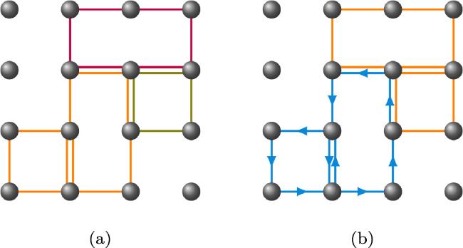
Figure 3. Typical graphical configurations for the O(3) spin model at different ℓ values: (a) For ℓ = 0, the configuration is composed of three copies of the Ising model graphs, as shown by orange, olive, and purple undirected lines, respectively; (b) for ℓ = 1, the configuration includes one copy of the XY model graph, denoted by the cyan directed lines, and an additional copy of the Ising model graph, represented by orange undirected lines. In both instances, each bond or site contributes a weight factor as specified in equations ( |
Furthermore, the partition function in the graphical description can be represented in tensor form as follows:
$\begin{eqnarray}{ \mathcal Z }=\displaystyle \sum _{\{{m}_{{ij}}^{\pm (\alpha )}\},\{{n}_{{ij}}^{(\beta )}\}}\displaystyle \prod _{i}{{\mathbb{T}}}^{(i)},\end{eqnarray}$
where the tensor ${{\mathbb{T}}}^{(i)}$ is defined as $\begin{eqnarray}\begin{array}{l}{{\mathbb{T}}}^{(i)}={ \mathcal I }(\{{k}_{i}^{(\alpha )}\},\{{l}_{i}^{(\beta )}\})\displaystyle \prod _{j\in {\mathbb{E}}(i)}\sqrt{W(\{{m}_{{ij}}^{\pm (\alpha )}\},\{{n}_{{ij}}^{(\beta )}\})}\\ \quad \cdot \displaystyle \prod _{\alpha }\delta ({{ \mathcal F }}^{(\alpha )})\,{\prod }_{\beta }\delta ({{ \mathcal L }}^{(\beta )}).\end{array}\end{eqnarray}$
Consequently, each graphical representation yields a corresponding tensor representation, marking the initial stride towards the application of the TNR method to the O(N) spin model.3. Worm algorithm
Based on the series of graphical representations derived in the previous section, we formulate worm algorithms to simulate the O(N) spin model for arbitrary N and ℓ. In these algorithms, starting from an arbitrary valid configuration, we introduce two defects named Ira and Masha into a randomly selected copy of an XY or Ising subgraph with a certain acceptance probability, causing the constraint in equation (22 ) to fail for the corresponding α or β of the selected subgraph at these two sites. In the defected subgraph, both Ira and Masha are connected by odd lines if it is an Ising subgraph, and one extra current flows in (out) for Ira (Masha) if it is an XY subgraph. To update the selected subgraph, we then move the defect Ira randomly by deleting (adding) a line or deleting (adding) a positive (negative) current, depending on whether it is an XY or Ising subgraph, until Ira meets Masha again.
We designate the space built by configurations with two defects as the ‘worm space'. Configurations within this space are weighted according to the two-point correlation function:
$\begin{eqnarray}\begin{array}{rcl}{ \mathcal Z }(I,M) & \equiv & \langle {{\boldsymbol{S}}}_{I}\cdot {{\boldsymbol{S}}}_{M}\rangle { \mathcal Z }\\ & = & \displaystyle \sum _{\alpha }{{ \mathcal Z }}_{{xy}}^{(\alpha )}(I,M)+\displaystyle \sum _{\beta }{{ \mathcal Z }}_{\mathrm{Is}}^{(\beta )}(I,M),\end{array}\end{eqnarray}$
where SI and SM represent the spin vectors at the sites Ira and Masha, respectively, and ${{ \mathcal Z }}_{{xy}}^{(\alpha )}(I,M)\equiv \langle {{\boldsymbol{S}}}_{I}^{(\alpha )}\cdot {{\boldsymbol{S}}}_{M}^{(\alpha )}\rangle \cdot { \mathcal Z }$ and ${{ \mathcal Z }}_{\mathrm{Is}}^{(\beta )}(I,M)\equiv \langle {{\boldsymbol{s}}}_{I}^{(\beta )}\cdot {{\boldsymbol{s}}}_{M}^{(\beta )}\rangle \cdot { \mathcal Z }$ denote the correlation functions for the respective decomposed spin vectors. They display the weights of the configurations when the defects are introduced into the corresponding subgraphs.Following the procedure outlined in section 2 , we can formulate the expansions of ${{ \mathcal Z }}_{{xy}}^{(\alpha )}(I,M)$ and ${{ \mathcal Z }}_{\mathrm{Is}}^{(\beta )}(I,M)$ in a manner similar to equation (21 ). These expansions follow the same bond weight factor formula as presented in equation (23 ), and adopt a similar formula for the site weight factor as seen in equation (24 ). In this case, ${{\boldsymbol{S}}}_{I/M}^{(\alpha )}$ or ${{\boldsymbol{s}}}_{I/M}^{(\beta )}$ within the angular brackets each contribute an additional +1 to the exponents of ${{ \mathcal A }}_{I/M,\alpha }$ or ${{ \mathcal B }}_{I/M,\beta }$ in the integration.
Due to the unitary modulus of the vector S, the correlation function ${ \mathcal Z }(I,M)$ simplifies to the partition function ${ \mathcal Z }$ when I = M. Thus, we can equivalently view configurations with both Ira and Masha on the same site as physical configurations. In this context, we can measure the observables on these configurations, disregarding the presence of both defects.
The procedures we use to update the Ising or XY subgraphs are identical to those employed for the Ising or XY model. A comprehensive description of the entire algorithm for a specific ℓ graphical representation can be found in algorithm 1 .
Algorithm 1. Worm algorithm for the O(N) spin model |
| if I = M then |
| Randomly choose a site $I^{\prime} $ from all sites in the lattice, and a copy of the subgraphs denoted as $\gamma ^{\prime} $ from ℓ copies of XY graphs and $N-2{\ell }$ copies of Ising graphs. |
| With the acceptance probability ${P}_{\gamma \to \gamma ^{\prime} }^{{acc}}(I\to I^{\prime} )$, set $I^{\prime} $ as the new location of both Ira and Masha, and change current modified subgraph to $\gamma ^{\prime} $, namely set $I=M=I^{\prime} $, $\gamma =\gamma ^{\prime} $. |
| end if |
| if γ is an XY subgraph then |
| Randomly select a site $I^{\prime} $ from all the nearest neighbor sites of site I. |
| If $I\to I^{\prime} $ is along the positive direction we selected in advance, set $\lambda =+1$, otherwise, set $\lambda =-1$. |
| Choose sgn to be + or − with equal probability. |
| Set ${m}_{{II}^{\prime} }^{{sgn}(\gamma )}={m}_{{II}^{\prime} }^{{sgn}(\gamma )}+\lambda \cdot {sgn}$ and move Ira to $I^{\prime} $, namely set $I=I^{\prime} $, with the acceptance probability ${P}_{\gamma ,{xy}}^{{acc}}(I\to I^{\prime} ,{sgn})$, unless this operation makes ${m}_{{II}^{\prime} }^{{sgn}(\gamma )}$ negative and is rejected directly. Here, sgn stands for +1 or −1 in the calculation correspondingly. |
| else |
| Randomly select a site $I^{\prime} $ from all the nearest neighbor sites of site I. |
| Select λ from +1 and −1 with equal probability. |
| Set ${n}_{{II}^{\prime} }^{(\gamma )}={n}_{{II}^{\prime} }^{(\gamma )}+\lambda $ and move Ira to $I^{\prime} $, namely set $I=I^{\prime} $, with the acceptance probability ${P}_{\gamma ,\mathrm{Is}}^{{acc}}(I\to I^{\prime} )$, unless this operation makes ${n}_{{II}^{\prime} }^{(\gamma )}$ negative and is rejected directly. |
| end if |
The specific expressions for the acceptance probabilities, ${P}_{\gamma \to \gamma ^{\prime} }^{{acc}}(I\to I^{\prime} )$, ${P}_{\gamma ,{xy}}^{{acc}}(I\to I^{\prime} ,{sgn})$ and ${P}_{\gamma ,\mathrm{Is}}^{{acc}}(I\to I^{\prime} )$, are provided in appendix B .
4. Numerical simulations
4.1. Setup
To probe the dynamical critical behavior of our worm algorithms, we conduct extensive simulations at the critical points for each N at various ℓ values. First, we introduce the observable we measure:
$\begin{eqnarray}{ \mathcal N }=\displaystyle \sum _{\langle i,j\rangle }\left(\displaystyle \sum _{\alpha }\left({m}_{{ij}}^{+(\alpha )}+{m}_{{ij}}^{-(\alpha )}\right)+\displaystyle \sum _{\beta }{n}_{{ij}}^{(\beta )}\right).\end{eqnarray}$
This observable counts all the lines in the graph, irrespective of their types. Intriguingly, the thermodynamic average of this quantity is effectively the negative of the system's energy, scaled by a temperature factor T, that is, $E=-T\langle { \mathcal N }\rangle $. This relationship can be readily confirmed by evaluating the formula $E=-\partial \mathrm{ln}Z/\partial K$.Based on the time series of the quantity ${ \mathcal N }$ in our Monte Carlo simulations, we compute the integrated autocorrelation time, ${\tau }_{\mathrm{int},{ \mathcal N }}$, which is defined as:
$\begin{eqnarray}{\tau }_{\mathrm{int},{ \mathcal N }}=\displaystyle \frac{1}{2}+\displaystyle \sum _{t=1}^{+\infty }{\rho }_{{ \mathcal N }}(t),\end{eqnarray}$
where t represents time, and ${\rho }_{{ \mathcal N }}(t)=(\langle {{ \mathcal N }}_{0}{{ \mathcal N }}_{t}\rangle -\langle { \mathcal N }{\rangle }^{2})/\mathrm{Var}({ \mathcal N })$ is the normalized autocorrelation function with variance given by $\mathrm{Var}({ \mathcal N })\equiv \langle {{ \mathcal N }}^{2}\rangle -\langle { \mathcal N }{\rangle }^{2}$. Given that an infinite time series is unattainable, we employ an upper truncation M for the summation in the calculation of ${\tau }_{\mathrm{int},{ \mathcal N }}$. Here, M is determined through a windowing method as described in appendix C of [15]: $\begin{eqnarray}M=\min \{m\in {\mathbb{N}}:m\geqslant c{\tau }_{\mathrm{int},{ \mathcal N }}(m)\},\end{eqnarray}$
where ${\tau }_{\mathrm{int},{ \mathcal N }}(m)\equiv 1/2+{\sum }_{t=1}^{m}{\rho }_{{ \mathcal N }}(t)$ and c represents the windowing parameter.In this study, we conduct simulations of systems at criticality for all possible values of ℓ across different N ranging from 2 to 6 on 3D cubic lattices with various system sizes L, extending up to 96. Periodic boundary conditions are implemented in all simulations. For every pair of N and L, we perform a total of 2 × 10⁸ measurements, with L/2 worm steps between two consecutive measurements. The critical couplings we use for each N are detailed in table 1.
Table 1. Critical couplings Kc we applied to simulate at for each N, and corresponding dynamical critical exponents ${z}_{\mathrm{int},{ \mathcal N }}$ at different ℓ which are roughly estimated via fitting the data by equation ( |
4.2. Results
We first examine the autocorrelation function ${\rho }_{{ \mathcal N }}(t)$ at the critical points Kc across various system sizes L for different N and ℓ values. As an illustrative example, figure 4 shows the variation of ${\rho }_{{ \mathcal N }}(t)$ as a function of time t for various system sizes L when N = 2. The figure reveals that for ℓ = 1, the decay of ${\rho }_{{ \mathcal N }}(t)$ nearly follows a pure exponential across all system sizes. However, for ℓ = 0, while the decay is approximately exponential for smaller L, the trend deviates from this behavior as L increases, leading to an intersection of lines representing ${\rho }_{{ \mathcal N }}(t)$ at different L around $t/{\tau }_{\mathrm{int},{ \mathcal N }}=3$. For N = 3, 4, 5, and 6, at all possible ℓ values, the behavior of ${\rho }_{{ \mathcal N }}(t)$ is akin to that observed for N = 2 and ℓ = 0. The underlying mechanism driving this phenomenon, however, remains unclear at present. A plausible scenario is that the decay of ${\rho }_{{ \mathcal N }}(t)$ is effectively the mixing of two exponential functions as ${\rho }_{{ \mathcal N }}(t)\approx {a}_{1}{{\rm{e}}}^{-t/{\tau }_{1}}+{a}_{2}{{\rm{e}}}^{-t/{\tau }_{2}}$. When exponents τ1 > τ2 and amplitudes a1 < a2, the decaying behavior of ${\rho }_{{ \mathcal N }}(t)$ is dominated by τ2 for small t but is eventually governed by τ1 for sufficiently large t.
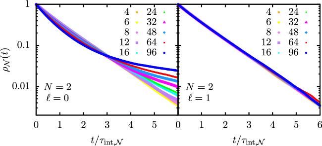
Figure 4. Autocorrelation function ${\rho }_{{ \mathcal N }}(t)$ at criticality versus $t/{\tau }_{\mathrm{int},{ \mathcal N }}$ for N = 2. At ℓ = 1, ${\rho }_{{ \mathcal N }}(t)$ is very close to a pure exponential decay, while at ℓ = 0, it exhibits a crossover from a pure exponential to a complicated behavior as L increases. |
Utilizing the formula in equation (30 ) and the truncation strategy, we derive the integrated autocorrelation time ${\tau }_{\mathrm{int},{ \mathcal N }}$ at criticality. Based on the patterns observed in ${\rho }_{{ \mathcal N }}(t)$, we select the windowing parameter c to be 8 for N = 2, ℓ = 1, and 20 for the remaining cases. Figure 5 presents the relationship between ${\tau }_{\mathrm{int},{ \mathcal N }}$ and system size for N = 2, while figure 6 depicts the same for N = 3, 4, 5 and 6. Across all N and ℓ values, ${\tau }_{\mathrm{int},{ \mathcal N }}$ appears to increase approximately as a power law with growing L, thereby indicating the manifestation of the critical slowing down phenomenon.
Figure 5. Integrated autocorrelation time ${\tau }_{\mathrm{int},{ \mathcal N }}$ at criticality versus system size L for N = 2. Here, ${\tau }_{\mathrm{int},{ \mathcal N }}$ is in the unit of one system sweep which equals to the number of bonds in the system. Blue and red points are for ℓ = 0 and 1, respectively. Dashed lines show the corresponding fitting results at large L with the fitting formula equation ( |
Figure 6. Integrated autocorrelation time ${\tau }_{\mathrm{int},{ \mathcal N }}$ at criticality for N = 3, 4, 5 and 6 at different ℓ, in the unit of system sweep. Points of different colors represent data for different ℓ, and dashed lines here have the same meaning as those in figure 5. |
To quantify this, we fit the data for ${\tau }_{\mathrm{int},{ \mathcal N }}$ at larger L values for all N and ℓ using the following formula:
$\begin{eqnarray}{\tau }_{\mathrm{int},{ \mathcal N }}={{AL}}^{{z}_{\mathrm{int},{ \mathcal N }}}.\end{eqnarray}$
The results of these fits are represented by the dashed lines in the corresponding figures, while the estimates for ${z}_{\mathrm{int},{ \mathcal N }}$ at different N and ℓ are detailed in table 1. The findings suggest that for each N, as ℓ increases, ${z}_{\mathrm{int},{ \mathcal N }}$ decreases monotonically, implying a higher efficiency of the worm algorithm at larger ℓ. This observation can also be directly gleaned from the slopes of each line in figures 5 and 6. Even for the worst case (ℓ = 0), the dynamic exponent z is significantly smaller than that for the Metropolis algorithm, which has z ≈ 2.0, meaning that the worm algorithms are much more efficient than the Metropolis method. In comparison with the Swendsen–Wang (SW) cluster method, which has z = 0.46(3) for the three-dimensional Ising model [12], the worm algorithm for the worst case (z ≲ 0.5) seems to be comparable, and for the best case (z ≲ 0.3) it seems to be somewhat more efficient, particularly for large N. Taking into account the existence of the ‘critical speeding-up' phenomenon for susceptibility-like quantities in worm-type simulations [21], we conclude that the worm algorithm is at least as efficient as the SW cluster method.5. Discussion
We present a successful reformulation of the O(N) spin model into a series of graphical representations, introduce corresponding worm algorithms to facilitate simulations and compare their dynamical critical behaviors. It is observed that the algorithm corresponding to the representation with a larger ℓ demonstrates a smaller dynamical critical exponent, implying a superior level of efficiency. Additionally, we employ these graphical representations to derive corresponding tensor representations, which we believe will be useful for TNR or other numerical methods.
The availability of multiple graphical representations allows us to investigate the underlying mechanisms contributing to the superior efficiency of these algorithms. This exploration provides valuable insights into their effective operation. To further enhance practical efficiency, our next step focuses on reducing the constant factor A of the autocorrelation time. We propose achieving this improvement by incorporating irreversible Monte Carlo techniques, specifically the lifting technique [22–25]. Our preliminary test verifies the potential of this approach, motivating its adoption in our research.
In addition to providing a series of new graphical representations and corresponding algorithms, our work presents a general idea for reformulating systems describing vectors with multiple components into graphical representations. This involves breaking the vectors into the sum of analogs with fewer components, which are easier to represent graphically. The configurations can then be decomposed into a coupling of corresponding subgraphs, opening up prospects for future graphical representations of the CP(N − 1) spin model.
Moreover, this approach can be applied to overcome the complex action problem when solving the O(N) spin model with a chemical potential μ coupled with conserved charges originating from the global O(N) symmetry [10]. By binding the components related to the chemical potential as a copy of the XY spin vector during the decomposition of the total spin vector, the chemical potential term can be reduced to an extra weight factor that depends on the conserved charges in the graphical representation. In this new representation, the positive and negative currents for the chemical-potential-related XY spin vector are no longer conserved unless the extra integer variables defined on each site that stand for the conserved charges are taken into account. It is also noted that these graphical representations can provide a convenient and effective platform to study many physical problems like universal conductivity or halon physics [26–28]. Overall, our approach offers a versatile tool to reformulate complex systems in a more accessible and intuitive graphical form.
Appendix A. Computation of equation (24 )
According to the restriction ${\sum }_{\alpha }{{ \mathcal A }}_{\alpha }^{2}+{\sum }_{\beta }{{ \mathcal B }}_{\beta }^{2}=1$, if we rewrite ${{ \mathcal B }}_{\beta }$ as ${{ \mathcal A }}_{{\ell }+\beta }$ (β = 1, 2, …, N − 2ℓ), we can express ${{ \mathcal A }}_{\alpha }$ in spherical coordinate system (θ1, θ2, …, θN−ℓ−1) as24 ) can be obtained directly.
$\begin{eqnarray}\left\{\begin{array}{l}{{ \mathcal A }}_{1}=\cos {\theta }_{1}\\ {{ \mathcal A }}_{2}=\sin {\theta }_{1}\cos {\theta }_{2}\\ \cdots \\ {{ \mathcal A }}_{N-{\ell }-1}=\sin {\theta }_{1}\sin {\theta }_{2}\cdots \sin {\theta }_{N-{\ell }-2}\cos {\theta }_{N-{\ell }-1}\\ {{ \mathcal A }}_{N-{\ell }}=\sin {\theta }_{1}\sin {\theta }_{2}\cdots \sin {\theta }_{N-{\ell }-2}\sin {\theta }_{N-{\ell }-1},\end{array}\right.\end{eqnarray}$
where θ1, θ2, …, θN−ℓ−1 ∈ [0, π/2]. It is standard that the surface element can be expressed as $\begin{eqnarray}\displaystyle \prod _{i=1}^{N-{\ell }}\hspace{-3pt}{\rm{d}}{{ \mathcal A }}_{i}{| }_{\displaystyle \sum _{\alpha =1}^{N-{\ell }}{{ \mathcal A }}_{\alpha }^{2}=1}\hspace{-3pt}=\hspace{-5pt}\displaystyle \prod _{i=1}^{N-{\ell }-2}\hspace{-5pt}{\sin }^{N-{\ell }-1-i}{\theta }_{i}\hspace{-5pt}\displaystyle \prod _{j=1}^{N-{\ell }-1}\hspace{-5pt}{\rm{d}}{\theta }_{j}.\end{eqnarray}$
By using the identity that $\begin{eqnarray}{\int }_{0}^{\tfrac{\pi }{2}}{\cos }^{x}\theta {\sin }^{y}\theta {\rm{d}}\theta =\displaystyle \frac{{\rm{\Gamma }}(\tfrac{x+1}{2}){\rm{\Gamma }}(\tfrac{y+1}{2})}{2{\rm{\Gamma }}(\tfrac{x+y+2}{2})},\end{eqnarray}$
where Γ( · ) is the Gamma function, equation (Appendix B. Acceptance probabilities
According to the Metropolis acceptance criterion, explicit expressions for ${P}_{\gamma \to \gamma ^{\prime} }^{\mathrm{acc}}(I\to I^{\prime} )=\min \{1,{q}^{(1)}\}$, ${P}_{\gamma ,{xy}}^{\mathrm{acc}}(I\to I^{\prime} ,{sgn})=\min \{1,{q}^{(2)}\}$ and ${P}_{\gamma ,\mathrm{Is}}^{\mathrm{acc}}(I\to I^{\prime} )=\min \{1,{q}^{(3)}\}$ are as follows:
| I | (I)For $(\gamma ,I)\to (\gamma ^{\prime} ,I^{\prime} )$: $\begin{eqnarray}{q}^{(1)}=\displaystyle \frac{{g}_{I}+N}{{g}_{I}^{(\gamma )}+f(\gamma )}\displaystyle \frac{{g}_{I^{\prime} }^{(\gamma ^{\prime} )}+f(\gamma ^{\prime} )}{{g}_{I^{\prime} }+N},\end{eqnarray}$ where $\begin{eqnarray}f(\gamma )=\left\{\begin{array}{cc}2, & \mathrm{if}\ \gamma \ \mathrm{is}\ \mathrm{an}\ \mathrm{XY}\ \mathrm{subgraph}\\ 1, & \mathrm{if}\ \gamma \ \mathrm{is}\ \mathrm{an}\ \mathrm{Ising}\ \mathrm{subgraph}\end{array}\right.,\end{eqnarray}$ $\begin{eqnarray}{g}_{I}^{(\gamma )}=\left\{\begin{array}{cc}{k}_{I}^{(\gamma )}, & \mathrm{if}\,\gamma \,\mathrm{is}\,\mathrm{an}\,\mathrm{XY}\,\mathrm{subgraph}\\ {l}_{I}^{(\gamma )}, & \mathrm{if}\,\gamma \,\mathrm{is}\,\mathrm{an}\,\mathrm{Ising}\,\mathrm{subgraph}\end{array}\right.,\end{eqnarray}$ and ${g}_{I}={\sum }_{\alpha }{k}_{I}^{(\alpha )}+{\sum }_{\beta }{l}_{I}^{(\beta )}$. The expressions of ${k}_{I}^{(\gamma )}$ and ${l}_{I}^{(\gamma )}$ are given by equation ( |
| II | (II)When γ is an XY subgraph: (i)${m}_{{II}^{\prime} }^{{sgn}(\gamma )}\to {m}_{{II}^{\prime} }^{{sgn}(\gamma )}+1$: $\begin{eqnarray}{q}^{(2)}=\displaystyle \frac{K}{2({m}_{{II}^{\prime} }^{{sgn}(\gamma )}+1)}\displaystyle \frac{{h}_{I^{\prime} }^{(\gamma )}+2}{{h}_{I^{\prime} }+N}\end{eqnarray}$ (ii)${m}_{{II}^{\prime} }^{{sgn}(\gamma )}\to {m}_{{II}^{\prime} }^{{sgn}(\gamma )}-1$: $\begin{eqnarray}{q}^{(2)}=\displaystyle \frac{2{m}_{{II}^{\prime} }^{{sgn}(\gamma )}}{K}\displaystyle \frac{{h}_{I}+N-2}{{h}_{I}^{(\gamma )}}.\end{eqnarray}$ |
| III | (III)When γ is an Ising subgraph: (i)${n}_{{II}^{\prime} }^{(\gamma )}\to {n}_{{II}^{\prime} }^{(\gamma )}+1$: $\begin{eqnarray}{q}^{(3)}=\displaystyle \frac{K}{{n}_{{II}^{\prime} }^{(\gamma )}+1}\displaystyle \frac{{h}_{I^{\prime} }^{(\gamma )}+1}{{h}_{I^{\prime} }+N}\end{eqnarray}$ (ii)${n}_{{II}^{\prime} }^{(\gamma )}\to {n}_{{II}^{\prime} }^{(\gamma )}-1$: $\begin{eqnarray}{q}^{(3)}=\displaystyle \frac{{n}_{{II}^{\prime} }^{(\gamma )}}{K}\displaystyle \frac{{h}_{I}+N-2}{{h}_{I}^{(\gamma )}-1}\end{eqnarray}$ |