


1. Introduction
The Poisson equation (PE) plays a key role in the field of electrostatics, where it is solved to determine electric potential from a provided charge distribution. The Poisson equation is linear in potential and is the source term used to stipulate the object's static electricity. Columb's law and Gauss's theorem derive the PE. The solution of the Poisson equation is actually a potential field subjected to a provided mass density distribution or electric charge and further, the determined potential field computes gravitational or electrostatic field. The Poisson equation models the phenomena of intersecting interfaces and electrodynamics [1, 2].
The field of local fractional calculus (LFC) investigates the characteristics of physical models appearing in a fractal space. Fractals appear as random geometrical structures that do not show any change during amplification of their shapes. The use of fractal theory can be found in various areas of physical sciences along with important applications in electrostatics, quantum mechanics and high energy physics. As compared to classical derivatives, a local fractional derivative (LFD) provides more precise estimates of performance measures. Fractals elucidate those images that cannot be undertaken by Euclidean geometry and handle those objects that deal with dimensions of real order. The nature of fractional-order modeling is nonlocal and therefore is irrelevant to deal with characteristics of local scaling phenomena or LF derivability. The LFD operator (LFDO) with fractal order is an efficient instrument for modeling physical phenomena and provides physical insights along with geometric observations. The motivational purpose of LFC is to explore the differential properties of extremely irregular & nondifferentiable functions. These LFDOs appeared as a generalized form of classical derivatives to fractal-order conserving local features of derivatives to explore local scaling properties of nowhere differentiable and extremely irregular functions [3]. These reasons and features prompted motivation for the modeling of the Poisson equation with LFDO. The above-discussed features of LFDs show the significance of the chosen local fractional Poisson equations (LFPEs) and that obviously, the local fractional modeling of the Poisson equation is far better and superior compared to integer- and fractional-order modeling of the Poisson equation.
When physical variables in Poisson's model are nondifferentiable functions defined on Cantor sets, the classical conservation law doesn't fit and so the integer-order Poisson's model becomes irrelevant in this sense. Therefore to deal with this difficulty, Chen et al [4] suggested the Poisson equation model with LFDO arising in electrostatistics within the LF conservation laws in the domain of LFC [5-7]. The Poisson equation with LFDO was presented in [4] as follows:
$\begin{eqnarray}\frac{{\partial }^{2\varepsilon }\varphi \left(\mu ,\tau \right)}{\partial {\mu }^{2\varepsilon }}+\frac{{\partial }^{2\varepsilon }\varphi \left(\mu ,\tau \right)}{\partial {\tau }^{2\varepsilon }}=h\left(\mu ,\tau \right),0\lt \varepsilon \leqslant 1\end{eqnarray}$
subject to the initial and boundary conditions: $\begin{eqnarray}\varphi \left(\mu ,0\right)=0,{\varphi }^{\left(\varepsilon \right)}\left(\mu ,0\right)=g\left(\mu \right)\end{eqnarray}$
where $\varphi \left(\mu ,\tau \right)$ is an unknown local fractional continuous nondifferentiable function, $g\left(\mu \right)$ is the given function, and the LFDO of $\varphi \left(\mu \right)$ of order $\varepsilon $ at $\mu ={\mu }_{0}$ is defined as $\begin{eqnarray}{\varphi }^{\left(\varepsilon \right)}\left({\mu }_{0}\right)=\mathop{\mathrm{lim}}\limits_{\mu \to {\mu }_{0}}\frac{{\unicode{x02206}}^{\varepsilon }\left(\varphi \left(\mu \right)-\varphi \left({\mu }_{0}\right)\right)}{{\left(\mu -{\mu }_{0}\right)}^{\varepsilon }},\end{eqnarray}$
where $\begin{eqnarray*}{\unicode{x02206}}^{\varepsilon }\left(\varphi \left(\mu \right)-\varphi \left({\mu }_{0}\right)\right)\cong {\rm{\Gamma }}\left(\varepsilon +1\right)\left(\varphi \left(\mu \right)-\varphi \left({\mu }_{0}\right)\right).\end{eqnarray*}$
Many analytical and numerical techniques have been employed to obtain approximate solutions of local fractional partial differential equations (LFPDEs) for example, the local fractional function decomposition method [8, 9], the local fractional Adomian decomposition technique (LFADT) [9-11], the local fractional series expansion technique [12, 13], the local fractional Laplace transform approach [14], the local fractional variational iteration approach (LFVIA) [15-19], the local fractional reduced differential transform scheme (LFRDTS) [19], the local fractional homotopy analysis Sumudu transform method [20], the local fractional differential transform scheme [21, 22], the local fractional Laplace VIA [23-28], the local fractional Laplace decomposition technique [29], the local fractional homotopy analysis scheme [30], the local fractional Laplace homotopy perturbation technique (LFLHPT) [31, 32] and the local fractional natural homotopy perturbation technique [33]. Recently, Dubey et al [34] and Kumar et al [35] presented fractal dynamics of LFPDEs occurring in physical sciences. Moreover, Dubey et al [36, 37] also investigated the local fractional Tricomi equation and local fractional Klein-Gordon models in a fractal media using hybrid local fractional schemes. Recently, Alqhtani et al [38] discussed spatiotemporal chaos in spatially extended fractional dynamical systems. Moreover, Alqhtani et al [39] studied the chaotic Lorenz system. Srivastava et al [40] analyzed fractal-fractional Kuramoto-Sivashinsky and Korteweg-de Vries equations.Recently, the LFPEs were studied by several authors using LFVIA [4], LFLHPT and LFRDTS [41]. Moreover, Singh et al [42] and Li et al [43] also studied and investigated the LFPEs in fractal media. The purpose of this paper is to introduce a new method to obtain the analytical approximate solutions to the Poisson equation with LFDO. In this paper, we apply the local fractional natural decomposition method (LFNDM) for the solution of LFPE. The LFNDM actually appears as a coupling of the LFADT [9, 44] and local fractional natural transform (LFNT) [33]. The LFNDM was introduced earlier in [45]. The main focus of the paper is to illustrate the implementation of LFNDM for different forms of LFPE and numerical simulations with the help of 3D graphic visuals on the cantor set. The LFPE explores the nature of the potential field in a fractal domain in view of nondifferentiable functions where a free charge occurs. The graphical analysis of the solution of LFPE provides significant physical characteristics of the LFPE in a fractal medium.
The application of the implemented method is shown by using two different examples and obtained solutions have also been compared with solutions computed by other methods in previous works. The 3D figures have been constructed for solutions of LFPE using MATLAB. The 3D plots depict the fractal nature of the function $\varphi \left(\mu ,\tau \right).$ The mathematical analysis shows that the implemented hybrid approach is beneficial to obtain the solutions for LFPEs. To make the convergence of LFNDM faster, the LFNT is selected. Two examples of LFPE are solved to demonstrate the application of LFNDM. The resulting solutions obtained from the applied scheme actually enter the picture as a special case of the classical Poisson equation model when the fractal order $\varepsilon =1,$ which shows the convergence of fractal geometry to Euclidean geometry. The coupling of LFADT with LFNT provides faster computations compared to the LFADT. Furthermore, this merger reduces the computational procedure as compared to other conventional methods while still giving reliable results. This work examines two significant aspects of the LFNDM. One feature is linked to the easy decomposition of non-linear quantities in a simple form by adopting Adomian polynomials and the other feature is related to the delivery of closed-form solutions in a series form with faster convergence. The original contributions of the paper are concerned with solution and numerical simulations for given LFPEs on the Cantor set via the applied hybrid method. It is also observed that the achieved solutions exactly match with previously reported solutions computed in the recent past.
The novelty and original contributions of the paper are applications of LFNDM to LFPEs which were constructed in [45]. Thus the new application along with computer simulations on the Cantorian set surely articulates the novelty of this work. The LFNDM provides fast convergence series solutions. The implemented method is time-saving, more trustable and proficient in comparison to other approaches. Moreover, computer-based simulations are also provided for the computed solutions of different forms of LFPE for the integer order $\varepsilon =1.0$ and the fractal order $\varepsilon =\frac{\mathrm{log}2}{\mathrm{log}3}$ of an LFD by using MATLAB. The remaining sections of the present work are developed as follows: In section 2 , some essential fundamentals of LFC are displayed. In section 3 , the basic procedure of LFNDM is provided. Applications of the LFNDM are demonstrated in section 4 . Section 5 deals with numerical simulations for LFPEs. The conclusion of the present paper is reported in section 6 .
2. Fundamentals of the LFC and LFNT
[46, 47]. The LF derivative of $\varphi (\mu )$ of order $\varepsilon $ at the point ${\mu }_{0}$ is defined as
$\begin{eqnarray}{\,\varphi }^{\left(\varepsilon \right)}\left({\tau }_{0}\right)=\mathop{\mathrm{lim}}\limits_{\mu \to {\mu }_{0}}\frac{{\rm{\Gamma }}\left(1+\varepsilon \right)\left[\varphi \left(\tau \right)-\varphi ({\tau }_{0})\right]}{{\left({\tau -\tau }_{0}\right)}^{\varepsilon }},0\lt \varepsilon \leqslant 1.\end{eqnarray}$
[47]. The Mittag-Leffler function in a fractal space is defined by
$\begin{eqnarray}{\,E}_{\varepsilon }\left({\tau }^{\varepsilon }\right)=\displaystyle \sum _{k=0}^{{\rm{\infty }}}\frac{{\tau }^{k\varepsilon }}{{\rm{\Gamma }}\left(1+k\varepsilon \right)},0\lt \varepsilon \leqslant 1.\end{eqnarray}$
[33]. The LFNT of a function $\varphi (\tau )$ of order $0\lt \varepsilon \leqslant 1$ is stated as
$\begin{eqnarray*}{\,{NT}}_{\varepsilon }\left\{\varphi \left(\tau \right)\right\}={{\rm{\unicode{x00424}}}}_{\varepsilon }\left(s,v\right)\end{eqnarray*}$$\begin{eqnarray}=\frac{1}{{\rm{\Gamma }}\left(1+\varepsilon \right)}{\int }_{0}^{{\rm{\infty }}}{E}_{\varepsilon }\left(\frac{-{s}^{\varepsilon }{\tau }^{\varepsilon }}{{v}^{\varepsilon }}\right)\frac{\varphi \left(\tau \right)}{{v}^{\varepsilon }}{(d\tau )}^{\varepsilon }.\end{eqnarray}$
Following (2.3 ), its inverse formula is expressed as
$\begin{eqnarray}{{NT}}_{\varepsilon }^{-1}\left[{{\rm{\unicode{x00424}}}}_{\varepsilon }\left(s,v\right)\right]=\frac{1}{{\left(2\pi i\right)}^{\varepsilon }}{\int }_{\gamma -i{\rm{\infty }}}^{\gamma +i{\rm{\infty }}}{E}_{\varepsilon }\left(\frac{{s}^{\varepsilon }{\tau }^{\varepsilon }}{{v}^{\varepsilon }}\right){{\rm{\unicode{x00424}}}}_{\varepsilon }\left(s,v\right){\left({\rm{d}}{s}\right)}^{\varepsilon },\end{eqnarray}$
where ${s}^{\varepsilon }$ and ${v}^{\varepsilon }$ are the local natural transform variables, and $\gamma $ is a real constant.The LFNT of some special functions reported in [33] are given as follows:
$\begin{eqnarray*}{\,{NT}}_{\varepsilon }\left\{\frac{{\tau }^{\varepsilon }}{{\rm{\Gamma }}\left(1+\epsilon \right)}\right\}=\frac{{v}^{\varepsilon }}{{s}^{2\varepsilon }},{\,{NT}}_{\varepsilon }\left\{{\sin }_{\varepsilon }\left({\tau }^{\varepsilon }\right)\right\}\end{eqnarray*}$
$\begin{eqnarray*}=\frac{{v}^{\varepsilon }}{{s}^{2\varepsilon }+{v}^{2\varepsilon }}{,{NT}}_{\varepsilon }\left\{{\cos }_{\varepsilon }{\rm{}}({\tau }^{\varepsilon })\right\}=\frac{{s}^{\varepsilon }}{{s}^{2\varepsilon }+{v}^{2\varepsilon }},\end{eqnarray*}$
$\begin{eqnarray*}{\,{NT}}_{\varepsilon }\left\{\frac{{\partial }^{m\varepsilon }\varphi \left(\mu ,\tau \right)}{{\partial \tau }^{m\varepsilon }}\right\}=\frac{{s}^{m\varepsilon }}{{v}^{m\varepsilon }}{{\rm{\unicode{x00424}}}}_{\varepsilon }\left(s,v\right)\end{eqnarray*}$
$\begin{eqnarray*}-\displaystyle \sum _{k=0}^{m-1}\frac{{s}^{\left(m-k-1\right)\varepsilon }}{{v}^{\left(m-k\right)\varepsilon }}\frac{{\partial }^{k\varepsilon }\varphi \left(\mu ,0\right)}{{\partial \tau }^{k\varepsilon }}.\end{eqnarray*}$
3. Analysis of LFNDM
To describe outlines of the procedure, the following partial differential equation (PDE) with LFDOs is considered
$\begin{eqnarray*}{L}_{\varepsilon }\varphi \left(\mu ,\tau \right)+{R}_{\varepsilon }\varphi \left(\mu ,\tau \right)\end{eqnarray*}$$\begin{eqnarray}+{F}_{\varepsilon }\varphi \left(\mu ,\tau \right)=g\left(\mu ,\tau \right),0\lt \varepsilon \leqslant 1,\end{eqnarray}$
where ${L}_{\varepsilon }=\frac{{\partial }^{m\varepsilon }}{\partial {\tau }^{m\varepsilon }},$ ${R}_{\varepsilon }$ denotes linear LFDO, ${F}_{\varepsilon }$ denotes nonlinear LFDO and $g\left(\mu ,\tau \right)$ is the nondifferentiable source ${\rm{i}}$ term.Operating the LFNT on equation (3.1 ) and using the property of the LFNT, we get
$\begin{eqnarray*}{\,{NT}}_{{\varepsilon }}\left\{{\varphi }\left({\mu },{\tau }\right)\right\}\end{eqnarray*}$$\begin{eqnarray*}=\displaystyle \sum _{{k}=0}^{{m}-1}\frac{{{v}}^{\left({m}-{k}-1\right){\varepsilon }}}{{{s}}^{\left({m}-{k}\right){\varepsilon }}}{{\varphi }}^{\left({k}{\varepsilon }\right)}\left({\mu },0\right)\end{eqnarray*}$$\begin{eqnarray*}+\frac{{{v}}^{{m}{\varepsilon }}}{{{s}}^{{m}{\varepsilon }}}{{NT}}_{{\varepsilon }}\left\{{g}\left({\mu },{\tau }\right)\right\}\end{eqnarray*}$$\begin{eqnarray}-\frac{{{v}}^{{m}{\varepsilon }}}{{{s}}^{{m}{\varepsilon }}}{{NT}}_{{\varepsilon }}\left\{{{R}}_{{\varepsilon }}{\varphi }\left({\mu },{\tau }\right)+{{F}}_{{\varepsilon }}{\varphi }\left({\mu },{\tau }\right)\right\}.\end{eqnarray}$
Applying the inverse formula of LFNT on equation (3.2 ), we acquire
$\begin{eqnarray*}{\varphi }\left({\mu },{\tau }\right)=\displaystyle \sum _{{k}=0}^{{m}-1}{{\varphi }}^{\left({k}{\varepsilon }\right)}\left({\mu },0\right)\frac{{{\tau }}^{{k}{\varepsilon }}}{{\rm{\Gamma }}\left(1+{k}{\varepsilon }\right)}\end{eqnarray*}$$\begin{eqnarray*}+{{NT}}_{{\varepsilon }}^{-1}\left[\frac{{{v}}^{{m}{\varepsilon }}}{{{s}}^{{m}{\varepsilon }}}{{NT}}_{{\varepsilon }}\left\{{g}\left({\mu },{\tau }\right)\right\}\right]\end{eqnarray*}$$\begin{eqnarray}-{{NT}}_{{\varepsilon }}^{-1}\left[\frac{{{v}}^{{m}{\varepsilon }}}{{{s}}^{{m}{\varepsilon }}}{{NT}}_{{\varepsilon }}\left\{{{R}}_{{\varepsilon }}{\varphi }\left({\mu },{\tau }\right)+{{F}}_{{\varepsilon }}{\varphi }\left({\mu },{\tau }\right)\right\}\right].\end{eqnarray}$
Now, we represent the solution in an infinite series in this way: $\begin{eqnarray}{\varphi }\left({\mu },{\tau }\right)=\displaystyle \sum _{{n}=0}^{{\rm{\infty }}}{{\varphi }}_{{n}}\left({\mu },{\tau }\right),\end{eqnarray}$
and the nonlinear term ${{F}}_{{\varepsilon }}{\varphi }\left({\mu },{\tau }\right)$ is written as $\begin{eqnarray}{{F}}_{{\varepsilon }}=\displaystyle \sum _{{n}=0}^{{\rm{\infty }}}{{A}}_{{n}}\left({\mu },{\tau }\right),\end{eqnarray}$
where ${{A}}_{{n}}$ is the local fractional Adomian polynomial and can be calculated using the following formula: $\begin{eqnarray*}{{A}}_{{n}}=\frac{1}{\Gamma \left(1+{n}{\varepsilon }\right)}\frac{{{\partial }}^{{n}{\varepsilon }}}{{\partial }{{\theta }}^{{n}{\varepsilon }}}\end{eqnarray*}$
$\begin{eqnarray*}\times {\left[{{F}}_{{\varepsilon }}\left(\displaystyle \sum _{{i}=0}^{{n}}{{{\theta }}^{{i}}\,{\varphi }}_{{i}}\left({\mu },{\tau }\right)\right)\right]}_{{\theta }=0},{n}=0,1,2.\end{eqnarray*}$
Using of equations (3.4 ) and (3.5 ) in equation (3.3 ) yields the following result: 3.6 ), we obtain
$\begin{eqnarray*}\displaystyle \sum _{{n}=0}^{{\rm{\infty }}}{{\varphi }}_{{n}}\left({\mu },{\tau }\right)\end{eqnarray*}$$\begin{eqnarray*}=\displaystyle \sum _{{k}=0}^{{m}-1}{{\varphi }}^{\left({k}{\varepsilon }\right)}\left({\mu },0\right)\frac{{{\tau }}^{{k}{\varepsilon }}}{{\rm{\Gamma }}\left(1+{k}{\varepsilon }\right)}\end{eqnarray*}$$\begin{eqnarray*}+{{NT}}_{{\varepsilon }}^{-1}\left[\frac{{{v}}^{{m}{\varepsilon }}}{{{s}}^{{m}{\varepsilon }}}{{NT}}_{{\varepsilon }}\left\{{g}\left({\mu },{\tau }\right)\right\}\right]\end{eqnarray*}$$\begin{eqnarray}-{{NT}}_{{\varepsilon }}^{-1}\left[\frac{{{v}}^{{m}{\varepsilon }}}{{{s}}^{{m}{\varepsilon }}}{{NT}}_{{\varepsilon }}\left\{{{R}}_{{\varepsilon }}\left[\displaystyle \sum _{{n}=0}^{{\rm{\infty }}}{{\varphi }}_{{n}}\left({\mu },{\tau }\right)\right]+\displaystyle \sum _{{n}=0}^{{\rm{\infty }}}{{A}}_{{n}}\left({\mu },{\tau }\right)\right\}\right].\end{eqnarray}$
On comparing both the sides of equation ( $\begin{eqnarray*}{{\varphi }}_{0}\left({\mu },{\tau }\right)=\displaystyle \sum _{{k}=0}^{{m}-1}{{\varphi }}^{\left({k}{\varepsilon }\right)}\left({\mu },0\right)\frac{{{\tau }}^{{k}{\varepsilon }}}{{\rm{\Gamma }}\left(1+{k}{\varepsilon }\right)}\end{eqnarray*}$$\begin{eqnarray*}+{{NT}}_{{\varepsilon }}^{-1}\left[\frac{{{v}}^{{m}{\varepsilon }}}{{{s}}^{{m}{\varepsilon }}}{{NT}}_{{\varepsilon }}\left\{{g}\left({\mu },{\tau }\right)\right\}\right],\end{eqnarray*}$$\begin{eqnarray*}{{\varphi }}_{1}\left({\mu },{\tau }\right)=-{{NT}}_{{\varepsilon }}^{-1}\left[\frac{{{v}}^{{m}{\varepsilon }}}{{{s}}^{{m}{\varepsilon }}}{{NT}}_{{\varepsilon }}\left\{{{R}}_{{\varepsilon }}\left[{{\varphi }}_{0}\left({\mu },{\tau }\right)\right]+{{A}}_{0}\right\}\right],\end{eqnarray*}$$\begin{eqnarray*}{{\varphi }}_{2}\left({\mu },{\tau }\right)=-{{NT}}_{{\varepsilon }}^{-1}\left[\frac{{{v}}^{{m}{\varepsilon }}}{{{s}}^{{m}{\varepsilon }}}{{NT}}_{{\varepsilon }}\left\{{{R}}_{{\varepsilon }}\left[{{\varphi }}_{1}\left({\mu },{\tau }\right)\right]+{{A}}_{1}\right\}\right],\end{eqnarray*}$$\begin{eqnarray*}{{\varphi }}_{3}\left({\mu },{\tau }\right)\end{eqnarray*}$$\begin{eqnarray}=-{{NT}}_{{\varepsilon }}^{-1}\left[\frac{{{v}}^{{m}{\varepsilon }}}{{{s}}^{{m}{\varepsilon }}}{{NT}}_{{\varepsilon }}\left\{{{R}}_{{\varepsilon }}\left[{{\varphi }}_{2}\left({\mu },{\tau }\right)\right]+{{A}}_{2}\right\}\right].\end{eqnarray}$
The local fractional recursive relation in its general form is obtained as 3.1 ) is given by
$\begin{eqnarray*}{{\varphi }}_{0}\left({\mu },{\tau }\right)=\displaystyle \sum _{{k}=0}^{{m}-1}{{\varphi }}^{\left({k}{\varepsilon }\right)}\left({\mu },0\right)\frac{{{\tau }}^{{k}{\varepsilon }}}{{\rm{\Gamma }}\left(1+{k}{\varepsilon }\right)}\end{eqnarray*}$$\begin{eqnarray*}+{{NT}}_{{\varepsilon }}^{-1}\left[\frac{{{v}}^{{m}{\varepsilon }}}{{{s}}^{{m}{\varepsilon }}}{{NT}}_{{\varepsilon }}\left\{{g}\left({\mu },{\tau }\right)\right\}\right],\end{eqnarray*}$$\begin{eqnarray*}{{\varphi }}_{{n}+1}\left({\mu },{\tau }\right)=-{{NT}}_{{\varepsilon }}^{-1}\left[\frac{{{v}}^{{m}{\varepsilon }}}{{{s}}^{{m}{\varepsilon }}}{{NT}}_{{\varepsilon }}\left\{{{R}}_{{\varepsilon }}\left[{{\varphi }}_{{n}}\left({\mu },{\tau }\right)\right]+{{A}}_{{n}}\right\}\right],\end{eqnarray*}$$\begin{eqnarray}{n}=0,1,2,3.\end{eqnarray}$
Hence, the approximation solution of equation ( $\begin{eqnarray}{\varphi }\left({\mu },{\tau }\right)=\displaystyle \sum _{{n}=0}^{{\rm{\infty }}}{{\varphi }}_{{n}}\left({\mu },{\tau }\right).\end{eqnarray}$
4. Applications of the LFNDM
Consider the following LFPE described in [41]
$\begin{eqnarray}\frac{{{\partial }}^{2{\varepsilon }}{\varphi }\left({\mu },{\tau }\right)}{{\partial }{{\mu }}^{2{\varepsilon }}}+\frac{{{\partial }}^{2{\varepsilon }}{\varphi }\left({\mu },{\tau }\right)}{{\partial }{{\tau }}^{2{\varepsilon }}}=\frac{{{\mu }}^{{\varepsilon }}}{\Gamma \left(1+{\varepsilon }\right)},0\lt {\varepsilon }\leqslant 1\,\end{eqnarray}$
with initial conditions:
$\begin{eqnarray}{\varphi }\left({\mu },0\right)=\frac{{{\mu }}^{3{\varepsilon }}}{\Gamma \left(1+3{\varepsilon }\right)},{{\varphi }}^{\left({\varepsilon }\right)}\left({\mu },0\right)={sin}_{{\varepsilon }}\left({{\mu }}^{{\varepsilon }}\right).\end{eqnarray}$
Using equations (3.8 ) and (4.1 ), the LF iteration algorithm is reported in the following form:
$\begin{eqnarray*}{{\varphi }}_{0}\left({\mu },{\tau }\right)=\frac{{{\mu }}^{3{\varepsilon }}}{\Gamma \left(1+3{\varepsilon }\right)}+\frac{{{\tau }}^{{\varepsilon }}}{\Gamma \left(1+{\varepsilon }\right)}{sin}_{{\varepsilon }}\left({{\mu }}^{{\varepsilon }}\right)\end{eqnarray*}$$\begin{eqnarray*}+\frac{{{\mu }}^{{\varepsilon }}}{\Gamma \left(1+{\varepsilon }\right)}\frac{{{\tau }}^{2{\varepsilon }}}{\Gamma \left(1+2{\varepsilon }\right)},\end{eqnarray*}$$\begin{eqnarray*}{{\varphi }}_{{n}+1}\left({\mu },{\tau }\right)=-{{NT}}_{{\varepsilon }}^{-1}\left[\frac{{{v}}^{2{\varepsilon }}}{{{s}}^{2{\varepsilon }}}{{NT}}_{{\varepsilon }}\left\{\frac{{{\partial }}^{2{\varepsilon }}}{{\partial }{{\mu }}^{2{\varepsilon }}}{{\varphi }}_{{n}}\left({\mu },{\tau }\right)\right\}\right],\end{eqnarray*}$$\begin{eqnarray}{n}=0,1,2.\end{eqnarray}$
From equation (4.3 ), we can find the following components
$\begin{eqnarray*}{{\varphi }}_{1}\left({\mu },{\tau }\right)=-{{NT}}_{{\varepsilon }}^{-1}\left[\frac{{{v}}^{2{\varepsilon }}}{{{s}}^{2{\varepsilon }}}{{NT}}_{{\varepsilon }}\left\{\frac{{{\partial }}^{2{\varepsilon }}}{{\partial }{{\mu }}^{2{\varepsilon }}}{{\varphi }}_{0}\left({\mu },{\tau }\right)\right\}\right]\end{eqnarray*}$
$\begin{eqnarray*}=-{{NT}}_{{\varepsilon }}^{-1}\left[\frac{{{v}}^{2{\varepsilon }}}{{{s}}^{2{\varepsilon }}}{{NT}}_{{\varepsilon }}\left\{\frac{{{\partial }}^{2{\varepsilon }}}{{\partial }{{\mu }}^{2{\varepsilon }}}\left(\frac{{{\mu }}^{3{\varepsilon }}}{\Gamma \left(1+3{\varepsilon }\right)}\right.\right.\right.\end{eqnarray*}$
$\begin{eqnarray*}\left.\left.\left.+\frac{{\tau }^{\varepsilon }}{\Gamma \left(1+\varepsilon \right)}{\sin }_{\varepsilon }\left({\mu }^{\varepsilon }\right)+\frac{{\mu }^{\varepsilon }}{\Gamma \left(1+\varepsilon \right)}\frac{{\tau }^{2\varepsilon }}{\Gamma \left(1+2\varepsilon \right)}\right)\right\}\right]\end{eqnarray*}$
$\begin{eqnarray*}=-{{NT}}_{{\varepsilon }}^{-1}\left[\frac{{{v}}^{2{\varepsilon }}}{{{s}}^{2{\varepsilon }}}{{NT}}_{{\varepsilon }}\left\{\frac{{{\mu }}^{{\varepsilon }}}{\Gamma \left(1+{\varepsilon }\right)}{-\frac{{{\tau }}^{{\varepsilon }}}{\Gamma \left(1+{\varepsilon }\right)}sin}_{{\varepsilon }}\left({{\mu }}^{{\varepsilon }}\right)\right\}\right]\end{eqnarray*}$
$\begin{eqnarray*}={-{NT}}_{{\varepsilon }}^{-1}\left[\frac{{{v}}^{2{\varepsilon }}}{{{s}}^{3{\varepsilon }}}\frac{{{\mu }}^{{\varepsilon }}}{\Gamma \left(1+{\varepsilon }\right)}-\frac{{{v}}^{3{\varepsilon }}}{{{s}}^{4{\varepsilon }}}{sin}_{{\varepsilon }}\left({{\mu }}^{{\varepsilon }}\right)\right]\end{eqnarray*}$
$\begin{eqnarray*}=-\frac{{{\mu }}^{{\varepsilon }}}{\Gamma \left(1+{\varepsilon }\right)}\frac{{{\tau }}^{2{\varepsilon }}}{\Gamma \left(1+2{\varepsilon }\right)}+\frac{{{\tau }}^{3{\varepsilon }}}{\Gamma \left(1+3{\varepsilon }\right)}{sin}_{{\varepsilon }}\left({{\mu }}^{{\varepsilon }}\right),\end{eqnarray*}$
$\begin{eqnarray*}{{\varphi }}_{2}\left({\mu },{\tau }\right)=-{{NT}}_{{\varepsilon }}^{-1}\left[\frac{{{v}}^{2{\varepsilon }}}{{{s}}^{2{\varepsilon }}}{{NT}}_{{\varepsilon }}\left\{\frac{{{\partial }}^{2{\varepsilon }}}{{\partial }{{\mu }}^{2{\varepsilon }}}{{\varphi }}_{1}\left({\mu },{\tau }\right)\right\}\right]\end{eqnarray*}$
$\begin{eqnarray*}=-{{NT}}_{{\varepsilon }}^{-1}\left[\frac{{{v}}^{2{\varepsilon }}}{{{s}}^{2{\varepsilon }}}{{NT}}_{{\varepsilon }}\left\{\frac{{{\partial }}^{2{\varepsilon }}}{{\partial }{{\mu }}^{2{\varepsilon }}}\left(-\frac{{{\tau }}^{2{\varepsilon }}}{\Gamma \left(1+2{\varepsilon }\right)}\frac{{{\mu }}^{{\varepsilon }}}{\Gamma \left(1+{\varepsilon }\right)}\right.\right.\right.\end{eqnarray*}$
$\begin{eqnarray*}\left.\left.\left.+\frac{{{\tau }}^{3{\varepsilon }}}{\Gamma \left(1+3{\varepsilon }\right)}{sin}_{{\varepsilon }}\left({{\mu }}^{{\varepsilon }}\right)\right)\right\}\right]\end{eqnarray*}$
$\begin{eqnarray*}=-{{NT}}_{{\varepsilon }}^{-1}\left[\frac{{{v}}^{2{\varepsilon }}}{{{s}}^{2{\varepsilon }}}{{NT}}_{{\varepsilon }}\left\{-\frac{{{\tau }}^{3{\varepsilon }}}{\Gamma \left(1+3{\varepsilon }\right)}{sin}_{{\varepsilon }}\left({{\mu }}^{{\varepsilon }}\right)\right\}\right]\end{eqnarray*}$
$\begin{eqnarray*}={{NT}}_{{\varepsilon }}^{-1}\left[\frac{{{v}}^{5{\varepsilon }}}{{{s}}^{6{\varepsilon }}}{sin}_{{\varepsilon }}\left({{\mu }}^{{\varepsilon }}\right)\right]\end{eqnarray*}$
$\begin{eqnarray*}=\frac{{{\tau }}^{5{\varepsilon }}}{\Gamma \left(1+5{\varepsilon }\right)}{sin}_{{\varepsilon }}\left({{\mu }}^{{\varepsilon }}\right),\end{eqnarray*}$
$\begin{eqnarray*}{{\varphi }}_{3}\left({\mu },{\tau }\right)=-{{NT}}_{{\varepsilon }}^{-1}\left[\frac{{{v}}^{2{\varepsilon }}}{{{s}}^{2{\varepsilon }}}{{NT}}_{{\varepsilon }}\left\{\frac{{{\partial }}^{2{\varepsilon }}}{{\partial }{{\mu }}^{2{\varepsilon }}}{{\varphi }}_{2}\left({\mu },{\tau }\right)\right\}\right]\end{eqnarray*}$
$\begin{eqnarray*}=-{{NT}}_{{\varepsilon }}^{-1}\left[\frac{{{v}}^{2{\varepsilon }}}{{{s}}^{2{\varepsilon }}}{{NT}}_{{\varepsilon }}\left\{\frac{{{\partial }}^{2{\varepsilon }}}{{\partial }{{\mu }}^{2{\varepsilon }}}\left(\frac{{{\tau }}^{5{\varepsilon }}}{\Gamma \left(1+5{\varepsilon }\right)}{sin}_{{\varepsilon }}\left({{\mu }}^{{\varepsilon }}\right)\right)\right\}\right]\end{eqnarray*}$
$\begin{eqnarray*}={-{NT}}_{{\varepsilon }}^{-1}\left[-\frac{{{v}}^{7{\varepsilon }}}{{{s}}^{8{\varepsilon }}}{sin}_{{\varepsilon }}\left({{\mu }}^{{\varepsilon }}\right)\right]\end{eqnarray*}$
$\begin{eqnarray*}=\frac{{{\tau }}^{7{\varepsilon }}}{\Gamma \left(1+7{\varepsilon }\right)}{sin}_{{\varepsilon }}\left({{\mu }}^{{\varepsilon }}\right)\end{eqnarray*}$
and so on.Therefore, the approximate solution ${\varphi }\left({\mu },{\tau }\right)$ of equation (4.1 ) is given by 4.4 ) is in good agreement with the solutions computed by LFLHPT and LFRDTS [41].
$\begin{eqnarray*}{\varphi }\left({\mu },{\tau }\right)=\displaystyle \sum _{{n}=0}^{{\rm{\infty }}}{{\varphi }}_{{n}}\left({\mu },{\tau }\right)\end{eqnarray*}$$\begin{eqnarray*}=\frac{{{\mu }}^{3{\varepsilon }}}{\Gamma \left(1+3{\varepsilon }\right)}\,\end{eqnarray*}$$\begin{eqnarray*}{+\,sin}_{{\varepsilon }}\left({{\mu }}^{{\varepsilon }}\right)\left(\frac{{\tau }^{\varepsilon }}{\Gamma \left(1+\varepsilon \right)}+\frac{{\tau }^{3\varepsilon }}{\Gamma \left(1+3\varepsilon \right)}+\frac{{\tau }^{5\varepsilon }}{\Gamma \left(1+5\varepsilon \right)}+\ldots \right)\end{eqnarray*}$$\begin{eqnarray}=\frac{{{\mu }}^{3{\varepsilon }}}{\Gamma \left(1+3{\varepsilon }\right)}+{sin}_{{\varepsilon }}\left({{\mu }}^{{\varepsilon }}\right){sinh}_{{\varepsilon }}\left({{\tau }}^{{\varepsilon }}\right).\end{eqnarray}$
The solution (We report the following LFPE described in [41]
$\begin{eqnarray}\frac{{{\partial }}^{2{\varepsilon }}{\varphi }\left({\mu },{\tau }\right)}{{\partial }{{\mu }}^{2{\varepsilon }}}+\frac{{{\partial }}^{2{\varepsilon }}{\varphi }\left({\mu },{\tau }\right)}{{\partial }{{\tau }}^{2{\varepsilon }}}={{E}}_{{\varepsilon }}\left({{\mu }}^{{\varepsilon }}\right),0\lt {\varepsilon }\leqslant 1\end{eqnarray}$
with initial conditions: $\begin{eqnarray}{\varphi }\left({\mu },0\right)={{E}}_{{\varepsilon }}\left({{\mu }}^{{\varepsilon }}\right),{{\varphi }}^{\left({\varepsilon }\right)}\left({\mu },0\right)={cos}_{{\varepsilon }}\left({{\mu }}^{{\varepsilon }}\right).\end{eqnarray}$
Making use of equations ( $\begin{eqnarray*}{{\varphi }}_{0}\left({\mu },{\tau }\right)={{E}}_{{\varepsilon }}\left({{\mu }}^{{\varepsilon }}\right)\,+\,\frac{{{\tau }}^{{\varepsilon }}}{\Gamma \left(1+{\varepsilon }\right)}{cos}_{{\varepsilon }}\left({{\mu }}^{{\varepsilon }}\right)\end{eqnarray*}$$\begin{eqnarray*}+\frac{{{\tau }}^{2{\varepsilon }}}{\Gamma \left(1+2{\varepsilon }\right)}{{E}}_{{\varepsilon }}\left({{\mu }}^{{\varepsilon }}\right),\end{eqnarray*}$$\begin{eqnarray*}{{\varphi }}_{{n}+1}\left({\mu },{\tau }\right)=-{{NT}}_{{\varepsilon }}^{-1}\end{eqnarray*}$$\begin{eqnarray}\left[\frac{{v}^{2\varepsilon }}{{s}^{2\varepsilon }}{{NT}}_{\varepsilon }\left\{\frac{{{\rm{\partial }}}^{2\varepsilon }}{{\rm{\partial }}{\mu }^{2\varepsilon }}{\varphi }_{n}\left(\mu ,\tau \right)\right\}\right],n=0,1,2.\end{eqnarray}$
From equation ( $\begin{eqnarray*}{{\varphi }}_{1}\left({\mu },{\tau }\right)=-{{NT}}_{{\varepsilon }}^{-1}\left[\frac{{{v}}^{2{\varepsilon }}}{{{s}}^{2{\varepsilon }}}{{NT}}_{{\varepsilon }}\left\{\frac{{{\partial }}^{2{\varepsilon }}}{{\partial }{{\mu }}^{2{\varepsilon }}}{{\varphi }}_{0}\left({\mu },{\tau }\right)\right\}\right]\end{eqnarray*}$
$\begin{eqnarray*}=-{{NT}}_{{\varepsilon }}^{-1}\left[\frac{{{v}}^{2{\varepsilon }}}{{{s}}^{2{\varepsilon }}}{{NT}}_{{\varepsilon }}\left\{\frac{{{\partial }}^{2{\varepsilon }}}{{\partial }{{\mu }}^{2{\varepsilon }}}\left({{E}}_{{\varepsilon }}\left({{\mu }}^{{\varepsilon }}\right){+\frac{{{\tau }}^{{\varepsilon }}}{\Gamma \left(1+{\varepsilon }\right)}cos}_{{\varepsilon }}\left({{\mu }}^{{\varepsilon }}\right)\right.\right.\right.\end{eqnarray*}$
$\begin{eqnarray*}\left.\left.\left.+\frac{{{\tau }}^{2{\varepsilon }}}{\Gamma \left(1+2{\varepsilon }\right)}{{E}}_{{\varepsilon }}\left({{\mu }}^{{\varepsilon }}\right)\right)\right\}\right]\end{eqnarray*}$
$\begin{eqnarray*}=-{{NT}}_{{\varepsilon }}^{-1}\left[\frac{{{v}}^{2{\varepsilon }}}{{{s}}^{2{\varepsilon }}}{{NT}}_{{\varepsilon }}\left\{{{E}}_{{\varepsilon }}\left({{\mu }}^{{\varepsilon }}\right)-\frac{{{\tau }}^{{\varepsilon }}}{\Gamma \left(1+{\varepsilon }\right)}{cos}_{{\varepsilon }}\left({{\mu }}^{{\varepsilon }}\right)\right.\right.\end{eqnarray*}$
$\begin{eqnarray*}\left.\left.+\frac{{{\tau }}^{2{\varepsilon }}}{\Gamma \left(1+2{\varepsilon }\right)}{{E}}_{{\varepsilon }}\left({{\mu }}^{{\varepsilon }}\right)\right\}\right]\end{eqnarray*}$
$\begin{eqnarray*}={-{NT}}_{{\varepsilon }}^{-1}\left[\frac{{{v}}^{2{\varepsilon }}}{{{s}}^{3{\varepsilon }}}{{E}}_{{\varepsilon }}\left({{\mu }}^{{\varepsilon }}\right)-\frac{{{v}}^{3{\varepsilon }}}{{{s}}^{4{\varepsilon }}}{cos}_{{\varepsilon }}\left({{\mu }}^{{\varepsilon }}\right)+\frac{{{v}}^{4{\varepsilon }}}{{{s}}^{5{\varepsilon }}}{{E}}_{{\varepsilon }}\left({{\mu }}^{{\varepsilon }}\right)\right]\end{eqnarray*}$
$\begin{eqnarray*}=-\frac{{{\tau }}^{2{\varepsilon }}}{\Gamma \left(1+2{\varepsilon }\right)}{{E}}_{{\varepsilon }}\left({{\mu }}^{{\varepsilon }}\right)+\frac{{{\tau }}^{3{\varepsilon }}}{\Gamma \left(1+3{\varepsilon }\right)}{cos}_{{\varepsilon }}\left({{\mu }}^{{\varepsilon }}\right)-\frac{{{\tau }}^{4{\varepsilon }}}{\Gamma \left(1+4{\varepsilon }\right)}{{E}}_{{\varepsilon }}\left({{\mu }}^{{\varepsilon }}\right),\end{eqnarray*}$
$\begin{eqnarray*}{{\varphi }}_{2}\left({\mu },{\tau }\right)=-{{NT}}_{{\varepsilon }}^{-1}\left[\frac{{{v}}^{2{\varepsilon }}}{{{s}}^{2{\varepsilon }}}{{NT}}_{{\varepsilon }}\left\{\frac{{{\partial }}^{2{\varepsilon }}}{{\partial }{{\mu }}^{2{\varepsilon }}}{{\varphi }}_{1}\left({\mu },{\tau }\right)\right\}\right]\end{eqnarray*}$
$\begin{eqnarray*}=-{{NT}}_{{\varepsilon }}^{-1}\left[\frac{{{v}}^{2{\varepsilon }}}{{{s}}^{2{\varepsilon }}}{{NT}}_{{\varepsilon }}\left\{\frac{{{\partial }}^{2{\varepsilon }}}{{\partial }{{\mu }}^{2{\varepsilon }}}\left(-\frac{{{\tau }}^{2{\varepsilon }}}{\Gamma \left(1+2{\varepsilon }\right)}{{E}}_{{\varepsilon }}\left({{\mu }}^{{\varepsilon }}\right)\right.\right.\right.\end{eqnarray*}$
$\begin{eqnarray*}\left.\left.\left.+\frac{{{\tau }}^{3{\varepsilon }}}{\Gamma \left(1+3{\varepsilon }\right)}{cos}_{{\varepsilon }}\left({{\mu }}^{{\varepsilon }}\right)-\frac{{{\tau }}^{4{\varepsilon }}}{\Gamma \left(1+4{\varepsilon }\right)}{{E}}_{{\varepsilon }}\left({{\mu }}^{{\varepsilon }}\right)\right)\right\}\right]\end{eqnarray*}$
$\begin{eqnarray*}=-{{NT}}_{{\varepsilon }}^{-1}\left[\frac{{{v}}^{2{\varepsilon }}}{{{s}}^{2{\varepsilon }}}{{NT}}_{{\varepsilon }}\left\{-\frac{{{\tau }}^{2{\varepsilon }}}{\Gamma \left(1+2{\varepsilon }\right)}{{E}}_{{\varepsilon }}\left({{\mu }}^{{\varepsilon }}\right)\right.\right.\end{eqnarray*}$
$\begin{eqnarray*}\left.\left.-\frac{{{\tau }}^{3{\varepsilon }}}{\Gamma \left(1+3{\varepsilon }\right)}{cos}_{{\varepsilon }}\left({{\mu }}^{{\varepsilon }}\right)-\frac{{{\tau }}^{4{\varepsilon }}}{\Gamma \left(1+4{\varepsilon }\right)}{{E}}_{{\varepsilon }}\left({{\mu }}^{{\varepsilon }}\right)\right\}\right]\end{eqnarray*}$
$\begin{eqnarray*}={-{NT}}_{{\varepsilon }}^{-1}\left[-\frac{{{v}}^{4{\varepsilon }}}{{{s}}^{5{\varepsilon }}}{{E}}_{{\varepsilon }}\left({{\mu }}^{{\varepsilon }}\right)-\frac{{{v}}^{5{\varepsilon }}}{{{s}}^{6{\varepsilon }}}\right.\end{eqnarray*}$
$\begin{eqnarray*}\times \left.{cos}_{{\varepsilon }}\left({{\mu }}^{{\varepsilon }}\right)+\frac{{{v}}^{6{\varepsilon }}}{{{s}}^{7{\varepsilon }}}{{E}}_{{\varepsilon }}\left({{\mu }}^{{\varepsilon }}\right)\right]\end{eqnarray*}$
$\begin{eqnarray*}=\frac{{{\tau }}^{4{\varepsilon }}}{\Gamma \left(1+4{\varepsilon }\right)}{{E}}_{{\varepsilon }}\left({{\mu }}^{{\varepsilon }}\right)+\frac{{{\tau }}^{5{\varepsilon }}}{\Gamma \left(1+5{\varepsilon }\right)}\end{eqnarray*}$
$\begin{eqnarray*}\times {cos}_{{\varepsilon }}\left({{\mu }}^{{\varepsilon }}\right)-\frac{{{\tau }}^{6{\varepsilon }}}{\Gamma \left(1+6{\varepsilon }\right)}{{E}}_{{\varepsilon }}\left({{\mu }}^{{\varepsilon }}\right).\end{eqnarray*}$
and so on.Therefore, the solution ${\varphi }\left({\mu },{\tau }\right)$ of equation (4.5 ) is given by
$\begin{eqnarray*}{\varphi }\left({\mu },{\tau }\right)=\displaystyle \sum _{{n}=0}^{{\rm{\infty }}}{{\varphi }}_{{n}}\left({\mu },{\tau }\right)={{E}}_{{\varepsilon }}\left({{\mu }}^{{\varepsilon }}\right){\,+\,cos}_{{\varepsilon }}\left({{\mu }}^{{\varepsilon }}\right)\end{eqnarray*}$$\begin{eqnarray*}\times \left(\frac{{\tau }^{\varepsilon }}{\Gamma \left(1+\varepsilon \right)}+\frac{{\tau }^{3\varepsilon }}{\Gamma \left(1+3\varepsilon \right)}+\frac{{\tau }^{5\varepsilon }}{\Gamma \left(1+5\varepsilon \right)}+\cdots \right)\end{eqnarray*}$$\begin{eqnarray}={{E}}_{{\varepsilon }}\left({{\mu }}^{{\varepsilon }}\right){\,+\,cos}_{{\varepsilon }}\left({{\mu }}^{{\varepsilon }}\right){sinh}_{{\varepsilon }}\left({{\tau }}^{{\varepsilon }}\right).\end{eqnarray}$
The acquired solution (4.8) is exactly the same as the solutions obtained by LFLHPT and LFRDTS [41].
5. Numerical results and analysis
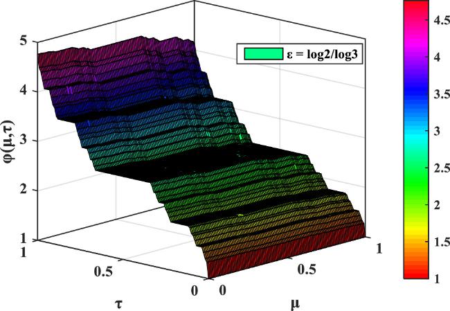
In this section, the computer-based simulations for solutions of LFPEs obtained by LFNDM are presented. The numerical investigation of LFPEs considers distinct values of $\varepsilon =1,\,\displaystyle \frac{\mathrm{log}\,2}{\mathrm{log}\,3}.$ Figures 1 and 2 elucidate the 3D variation of solution $\phi \left(\mu ,\,\tau \right)$ for Example 1 for $\varepsilon =1.0$ and $\varepsilon =\,\displaystyle \frac{\mathrm{log}\,2}{\mathrm{log}\,3},$ respectively. Similarly, figures 3 and 4, respectively, demonstrate the nature of $\phi \left(\mu ,\,\tau \right)$ for Example 2 for $\varepsilon =1.0$ and $\varepsilon =\,\displaystyle \frac{\mathrm{log}\,2}{\mathrm{log}\,3}.$ Figures 2 and 4, respectively, depict the variation of $\phi \left(\mu ,\,\tau \right)$ in a fractal domain for Examples 1 and 2. The graphic visuals for the solution $\phi \left(\mu ,\,\tau \right)$ demonstrate a fractal nature and obviously depict the nondifferentiability of the function in certain phases.

Figure 1. 3D plot of $\phi \left(\mu ,\,\tau \right)$ for Example 1 with respect to $\mu $ and $\tau $ for $\varepsilon =1.0.$ |
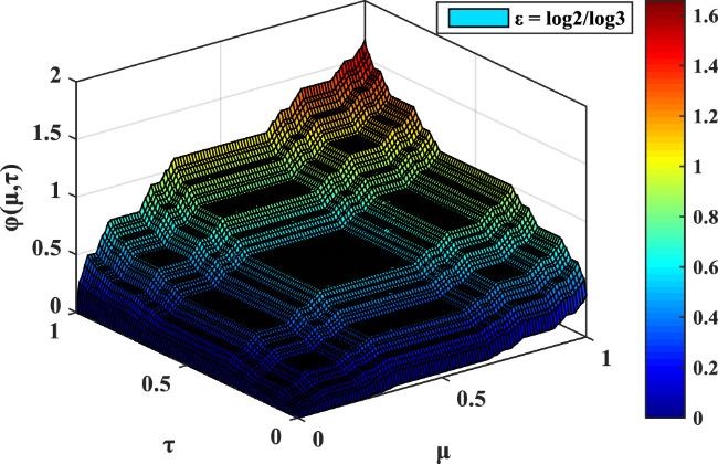
Figure 2. 3D variation of $\phi \left(\mu ,\,\tau \right)$ for Example 1 with respect to $\mu $ and $\tau $ for $\varepsilon =\displaystyle \frac{\mathrm{log}\,2}{\mathrm{log}\,3}.$ |

Figure 3. 3D plot of $\phi \left(\mu ,\,\tau \right)$ for Example 2 with respect to $\mu $ and $\tau $ for $\varepsilon =1.0.$ |
Figure 4. 3D plot of $\phi \left(\mu ,\,\tau \right)$ for Example 2 with respect to $\mu $ and $\tau $ for $\varepsilon =\,\mathrm{log}\,2/\,\mathrm{log}\,3.$ |
6. Conclusion
In this work, we have considered the LFPE with LFDOs. The method which is called the LFNDM has been applied successfully to attain the approximate solutions for LFPEs. The results are obtained in the closed form of an infinite power series. The examples show that the outcomes of LFNDM are in good agreement with the results obtained by LFLHPT and LFRDTS. This work also depicts that the applied method is systematic and can be helpful for solving nonlinear and linear LFPDEs with fractal order. In future studies, other fractal order physical models can also be solved by the applied technique to attain new results and conclusions.