


1. Introduction
The study of analytical solutions helps us to clarify the physical properties and behaviour of nonlinear equations, which are structural models for many physical phenomena [1]. There are a number of theoretical approaches to solving analytical solutions, such as the tanh-coth method [2-4], Riemann-Hilbert method [5-7], the inverse scattering method [8, 9], Darboux transformation method [10-13], the Painlevé analysis [14], the generalized symmetry method [15], Hirota bilinear method [16, 17, 38] and others [18-21].
In the subject area of the natural sciences, solitons demonstrate remarkable order in the presence of nonlinear effects. In general, we refer to a wave that retains its original size, shape and direction during motion or propagation, and has stability, as a soliton wave [22]. In recent years, a new topic soliton molecules has emerged in the study of solitons, which are bound states of one or more solitons [23-27, 41-43]. The three well-known local waves: lump waves, breathers and line waves are very significant components of soliton molecule solutions.
The (3+1)-dimensional Jimbo-Miwa equation2 ) belongs to the Kadomtsev-Petviashvili hierarchy, but it does not satisfy the classical productability condition [28].
$\begin{eqnarray}\begin{array}{l}{u}_{{xxxy}}^{}+3{u}_{{xy}}^{}{u}_{x}^{}+3{u}_{y}^{}{u}_{{xx}}^{}\\ +2{u}_{{yt}}^{}-3{u}_{{xz}}^{}=0,\end{array}\end{eqnarray}$
first introduced by Jimbo and Miwa [28] is the second equation of the KP hierarchy. This equation is used to describe certain interesting (3+1)-dimensional waves in physics and then discussed by many authors on its solutions [29], integrability properties [30], symmetries [31-33] and so on. Wazwaz have proposed two extended (3+1)-dimensional Jimbo-Miwa (3D-eJM) equations [34]. The second 3D-eJM equation is deduced by replacing ${u}_{{yt}}^{}$ with ${u}_{{xt}}^{}+{u}_{{yt}}^{}+{u}_{{zt}}^{}$ as $\begin{eqnarray}\begin{array}{l}{u}_{{xxxy}}^{}+3{u}_{{xy}}^{}{u}_{x}^{}+3{u}_{y}^{}{u}_{{xx}}^{}+2{u}_{{xt}}^{}\\ +2{u}_{{yt}}^{}+2{u}_{{zt}}^{}-3{u}_{{xz}}^{}=0,\end{array}\end{eqnarray}$
where u = u(x, y, z, t) is a function with respect to three spatial coordinates x, y, z and temporal variable t which indicates the amplitude of the wave in the physics of fluids, especially in ocean engineering and science [1]. Although equation (In contrast to other 3D-eJM equation, relatively little research has been done on this equation. For equation (2 ), Wazwaz derived multiple soliton solutions [34], Guo et al presented four different localized waves and interaction solutions between lump solutions, line solitons, breathers and rogue waves using the Hirota bilinear method, Sun et al found lump and lump-kink solution [36], Xu et al constructed the resonance behavior with the aid of special parameter restrictions [37]. But as far as we know, no molecule solution of this equation has been studied, especially for the lump molecule solution, a special structural phenomenon that does not exist in most (2+1)-dimensional physical models by using long wave limit method [38, 39]. All of findings in this paper can be used to explain some natural phenomena in the ocean waves and nonlinear optics. Further, the study can be extended to investigate several other nonlinear systems to understand the physical insights of the molecule phenomenon in their dynamics.
This paper has following structure. In section 2 , we give four different types of localized waves and the expression of their velocity through the use of N-soliton solution, module and velocity resonance conditions, long wave limit method. We present three molecule solutions consisting of the same localized wave e.g: line molecule, breather molecule and lump molecule solution in section 3 . In section 4 , a number of molecule solutions with a mixture of different localized waves are obtained. And two forms of the higher order line molecule solutions are derived. Some conclusions and discussions are given in section 5 .
2. Different localized waves to the second 3D-eJM equation
According to the Hirota bilinear method and Bell polynomial technique, with logarithmic transform2 ) can be converted to following bilinear form:4 ) can be expanded as4 ) has the following form:2 ) can be expressed through substituting equation (6 ) into equation (3 ). Based on the N-soliton solution, we construct a number of different localized waves.
$\begin{eqnarray}u(x,y,z,t)=2\displaystyle \frac{\partial }{{\partial }_{x}}\mathrm{ln}f(x,y,z,t),\end{eqnarray}$
the equation ( $\begin{eqnarray}\begin{array}{l}({D}_{x}^{3}{D}_{y}+2{D}_{x}{D}_{t}+2{D}_{y}{D}_{t}+2{D}_{z}{D}_{t}-3{D}_{x}{D}_{z})\\ \times (f\cdot f)=0,\end{array}\end{eqnarray}$
where operators Dx, Dt are defined by $\begin{eqnarray}\begin{array}{l}{D}_{x}^{p}{D}_{t}^{q}(f\cdot g)={\left(\displaystyle \frac{\partial }{\partial x}-\displaystyle \frac{\partial }{\partial {x}^{{\prime} }}\right)}^{p}{\left(\displaystyle \frac{\partial }{\partial t}-\displaystyle \frac{\partial }{\partial {t}^{{\prime} }}\right)}^{q}{\left.\,\left(f(x,t)\cdot g({x}^{{\prime} },{t}^{{\prime} })\right)\right|}_{x={x}^{{\prime} },t={t}^{{\prime} }}.\end{array}\end{eqnarray}$
To facilitate mathematical calculations, the equation ( $\begin{eqnarray*}\begin{array}{l}{f}_{{\text{xxxy}}}f-{f}_{{\text{xxx}}}{f}_{y}-3{f}_{{\text{xxy}}}{f}_{x}\\ +3{f}_{{\text{xx}}}{f}_{{\text{xy}}}+2{f}_{}{f}_{{\text{xt}}}-2{f}_{t}{f}_{x}\\ +2{f}_{}{f}_{{\text{yt}}}-2{f}_{t}{f}_{y}+2{f}_{}{f}_{{\text{zt}}}\\ -2{f}_{t}{f}_{z}-3{{ff}}_{{\text{xz}}}+3{f}_{z}{f}_{x}=0.\end{array}\end{eqnarray*}$
The N order solution of equation ( $\begin{eqnarray}f={f}_{N}={\sum }_{\mu =0,1}^{}\exp \left({\sum }_{k=1}^{N}{\mu }_{k}{\xi }_{k}+{\sum }_{k\lt s}^{N}{\mu }_{k}{\mu }_{s}{A}_{{ks}}\right),\end{eqnarray}$
where $\begin{eqnarray}\begin{array}{rcl}{\xi }_{k} & = & \ {p}_{k}^{}x+{q}_{k}^{}y+{r}_{k}^{}z+{\omega }_{k}^{}t+{\phi }_{k}^{},{\omega }_{k}^{}\\ & = & -\displaystyle \frac{{p}_{k}^{3}{q}_{k}^{}-3{p}_{k}^{}{r}_{k}^{}}{2({p}_{k}^{}+{q}_{k}^{}+{r}_{k}^{})},{A}_{{ks}}^{}=\mathrm{ln}\left(\displaystyle \frac{M}{N}\right),\\ M & = & \ {p}_{k}^{4}{q}_{s}\left({p}_{s}^{}+{q}_{s}^{}+{r}_{s}^{}\right)+{p}_{k}^{3}\left({p}_{s}^{}+{q}_{s}^{}+{r}_{s}^{}\right)\\ & & \times \left(2{p}_{s}^{}{q}_{k}^{}-3{p}_{s}^{}{q}_{s}^{}+{q}_{s}^{}{r}_{k}^{}-{q}_{k}^{}{r}_{s}^{}\right)\\ & & +{p}_{k}^{2}\left[{p}_{s}^{3}\left(2{q}_{s}^{}-3{q}_{k}^{}\right)+3{p}_{s}^{2}\left({q}_{k}^{}-{q}_{s}^{}\right)\left({q}_{k}^{}-{q}_{s}^{}+{r}_{k}^{}-{r}_{s}^{}\right)\right.\\ & & +\,3{p}_{s}^{}\left({q}_{k}^{}-{q}_{s}^{}\right)\left({q}_{k}^{}+{r}_{k}^{}\right)\\ & & \quad \left.\left({q}_{s}^{}+{r}_{s}^{}\right)-3{r}_{s}^{}\left({q}_{s}^{}+{r}_{s}^{}\right)\right]+{p}_{s}^{3}{p}_{k}^{}\left[{r}_{s}^{}{q}_{k}^{}+{r}_{k}^{}{q}_{s}^{}\right.\\ & & \left.+2{q}_{k}^{}{q}_{s}^{}-3{q}_{k}^{}\left({q}_{k}^{}+{r}_{k}^{}\right)\right]+{p}_{k}^{}{p}_{s}^{4}{q}_{k}^{}\\ & & -3{p}_{k}^{}{p}_{s}^{2}\left({q}_{k}^{}-{q}_{s}^{}\right)\left({q}_{k}^{}+{r}_{k}^{}\right)\left({q}_{s}^{}+{r}_{s}^{}\right)\\ & & +3{p}_{k}^{}{p}_{s}^{}\left({q}_{k}^{}{r}_{s}^{}+{q}_{s}^{}{r}_{k}^{}+2{r}_{k}^{}{r}_{s}^{}\right)-3{p}_{k}^{}\left({q}_{k}^{}{r}_{s}^{}-{q}_{s}^{}{r}_{k}^{}\right)\\ & & \quad \left({q}_{s}^{}+{r}_{s}^{}\right)+{p}_{s}^{}\left({q}_{k}^{}+{r}_{k}\right)\\ & & \times \left[{p}_{s}^{3}{q}_{k}^{}+\left({p}_{s}^{2}+3\right)\left({q}_{k}^{}{r}_{s}^{}-{q}_{s}^{}{r}_{k}^{}\right)-3{p}_{s}^{}{r}_{k}\right],\\ N & = & \ {p}_{k}^{4}{q}_{s}\left({p}_{s}^{}+{q}_{s}^{}+{r}_{s}^{}\right)+{p}_{k}^{3}\left({p}_{s}^{}+{q}_{s}^{}+{r}_{s}^{}\right)\\ & & \times \left(2{p}_{s}^{}{q}_{k}^{}+3{p}_{s}^{}{q}_{s}^{}+{q}_{s}^{}{r}_{k}^{}-{q}_{k}^{}{r}_{s}^{}\right)\\ & & +{p}_{k}^{2}\left[{p}_{s}^{3}\left(2{q}_{s}^{}+3{q}_{k}^{}\right)+3{p}_{s}^{2}\left({q}_{k}^{}+{q}_{s}^{}\right)\left({q}_{k}^{}+{q}_{s}^{}+{r}_{k}^{}+{r}_{s}^{}\right)+3{p}_{s}^{}\left({q}_{k}^{}+{q}_{s}^{}\right)\left({q}_{k}^{}+{r}_{k}^{}\right)\right.\\ & & \times \left.\left({q}_{s}^{}+{r}_{s}^{}\right)-3{r}_{s}^{}\left({q}_{s}^{}+{r}_{s}^{}\right)\right]+{p}_{s}^{3}{p}_{k}^{}\left[{r}_{s}^{}{q}_{k}^{}\right.\\ & & \left.+{r}_{k}^{}{q}_{s}^{}+2{q}_{k}^{}{q}_{s}^{}+3{q}_{k}^{}\left({q}_{k}^{}+{r}_{k}^{}\right)\right]+{p}_{k}^{}{p}_{s}^{4}{q}_{k}^{}\\ & & +3{p}_{k}^{}{p}_{s}^{2}\left({q}_{k}^{}+{q}_{s}^{}\right)\left({q}_{k}^{}+{r}_{k}^{}\right)\left({q}_{s}^{}+{r}_{s}^{}\right)+3{p}_{k}^{}{p}_{s}^{}\\ & & \times \left({q}_{k}^{}{r}_{s}^{}+{q}_{s}^{}{r}_{k}^{}+2{r}_{k}^{}{r}_{s}^{}\right)-3{p}_{k}^{}\left({q}_{k}^{}{r}_{s}^{}-{q}_{s}^{}{r}_{k}^{}\right)\\ & & \times \left({q}_{s}^{}+{r}_{s}^{}\right)+{p}_{s}^{}\left({q}_{k}^{}+{r}_{k}\right)\\ & & \times \left[{p}_{s}^{3}{q}_{k}^{}+\left({p}_{s}^{2}+3\right)\left({q}_{k}^{}{r}_{s}^{}-{q}_{s}^{}{r}_{k}^{}\right)-3{p}_{s}^{}{r}_{k}\right].\end{array}\end{eqnarray}$
Here, ${p}_{k}^{},{q}_{k}^{},{r}_{k}^{},{\phi }_{k}(k=1,2,\cdots ,N)$ are arbitrary constants, ∑μ=0,1 denotes all combinations of μk = 0 or 1. The N-soliton solution of equation (Figures 1(a), (b) depicts the 3D-plot and density plot of single line soliton with parameters p1 = 1, q1 = 1, r1 = 2, φ1 = 0 at z = 0 plane. Subject to this parameter, equation (3 ) is reduced to7 ). The velocity of single line wave in equation (8 ) is $\left(-\tfrac{5}{16},-\tfrac{5}{16}\right)$. The correctness of the above assertion can be demonstrated in figure 1(b).
$\begin{eqnarray}u(x,y,z,t)=\displaystyle \frac{2{{\rm{e}}}^{x+y+\tfrac{5}{8}t}}{1+{{\rm{e}}}^{x+y+\tfrac{5}{8}t}}.\end{eqnarray}$
Actually the ratio of p1 to −q1 determines the slope of the line in figure 1(b), φ1 affects the initial position (t = 0) of the solution in the diagram. In other words, if φ1 is not equal to zero, then the centre of the solution at the initial position must not pass through (0, 0) at z = 0. In order to better study the motion of line wave, we decompose the velocity of the solution orthogonally in the x, y perpendicular directions and give its expression as follows $\begin{eqnarray}\begin{array}{rcl}{V}_{\mathrm{line}} & = & \left({V}_{x},{V}_{y}\right)=\left(-\displaystyle \frac{{\omega }_{k}^{}{p}_{k}^{}}{{p}_{k}^{2}+{q}_{k}^{2}},-\displaystyle \frac{{\omega }_{k}^{}{q}_{k}^{}}{{p}_{k}^{2}+{q}_{k}^{2}}\right),\\ k & = & 1,2,\cdots ,N,\end{array}\end{eqnarray}$
where ${\omega }_{k}^{}$ satisfies equation (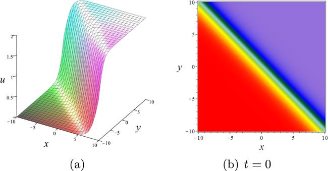
Figure 1. Single soliton solution to the 3D-eJM equation with p1 = 1, q1 = 1, r1 = 2, φ1 = 0, z = 0 in equation ( |
Double soliton solution can be seen as a morphism consisting of the nonlinear superposition of two single soliton solutions. Its kinematic process can be split into two mutually independent single line wave motions and its velocity can be elaborated by two velocity expressions in equation (9 ). This also indicates that the collision between two soliton waves is elastic: the velocity, phase shift and amplitude do not change before or after the collision. With p1 = 1, q1 = 1, r1 = 2, p2 = 2, q2 = 4, r2 = 1, φ1 = φ2 = 0, a double soliton solution to the 3D-eJM equation is presented as
$\begin{eqnarray}\begin{array}{l}u(x,y,z,t)\\ =\,\displaystyle \frac{2\left(755{{\rm{e}}}^{x+y+\tfrac{5t}{8}}+1510{{\rm{e}}}^{2x+4y-\tfrac{13t}{7}}+249{{\rm{e}}}^{3x+5y-\tfrac{69t}{56}}\right)}{755+755{{\rm{e}}}^{x+y+\tfrac{5t}{8}}+755{{\rm{e}}}^{2x+4y-\tfrac{13t}{7}}+83{{\rm{e}}}^{3x+5y-\tfrac{69t}{56}}}.\end{array}\end{eqnarray}$
It can be seen in figure 2 and travels at a speed of $\left(-\tfrac{5}{16},-\tfrac{5}{16}\right)$, $\left(\tfrac{13}{70},\tfrac{13}{35}\right)$.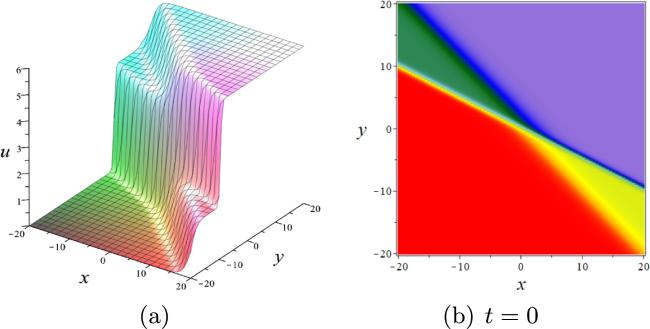
Figure 2. Double soliton solution to the 3D-eJM equation with p1 = 1, q1 = 1, r1 = 2, p2 = 2, q2 = 4, r2 = 1, φ1 = φ2 = 0, z = 0 in equation ( |
The N-order breather solution can be obtained by imposing module resonance condition on the parameters of the 2N-order soliton solution, i.e.
$\begin{eqnarray}\begin{array}{rcl}{p}_{1}^{} & = & {p}_{2}^{* },{q}_{1}^{}={q}_{2}^{* },\\ {r}_{1}^{} & = & {r}_{2}^{* },{\phi }_{1}={\phi }_{2},\cdots ,\\ {p}_{2N-1}^{} & = & {p}_{2N}^{* },{q}_{2N-1}^{}={q}_{2N}^{* },\\ {r}_{2N-1}^{} & = & {r}_{2N}^{* },{\phi }_{2N-1}={\phi }_{2N},\end{array}\end{eqnarray}$
where the symbol * indicates the complex conjugate number of the parameter. It is similar in nature since the breather solution is derived from the soliton solution. But the pace expression of breather is $\begin{eqnarray}\begin{array}{l}{V}_{\mathrm{breather}}=\left({V}_{x},{V}_{y}\right)\\ =\,\left(-\displaystyle \frac{{\mathfrak{R}}({\omega }_{k}^{}){\mathfrak{R}}({p}_{k}^{})}{{\mathfrak{R}}{\left({p}_{k}^{}\right)}^{2}+{\mathfrak{R}}{\left({q}_{k}^{}\right)}^{2}},-\displaystyle \frac{{\mathfrak{R}}({\omega }_{k}^{}){\mathfrak{R}}({q}_{k}^{})}{{\mathfrak{R}}{\left({p}_{k}^{}\right)}^{2}+{\mathfrak{R}}{\left({q}_{k}^{}\right)}^{2}}\right),\\ k=1,3,\cdots ,2N-1.\end{array}\end{eqnarray}$
For N = 1, a first order line breather solution is shown in figure 3 by selecting ${p}_{1}^{}={p}_{2}^{* }=i$, ${q}_{1}^{}={q}_{2}^{* }=1$, ${r}_{1}^{}={r}_{2}^{* }=2+i,z\,=0,t=0,{\phi }_{1}={\phi }_{2}=0$. It moves with speed $\tfrac{5}{26}$ along the negative direction of the y-axis.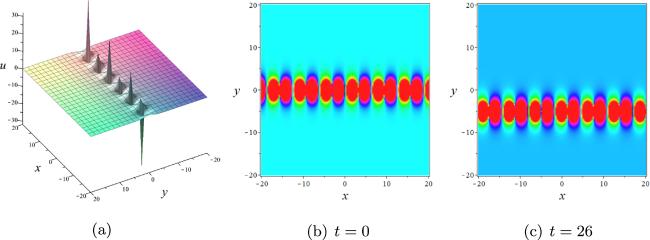
Figure 3. First order line breather solution to the 3D-eJM equation with ${p}_{1}^{}={p}_{2}^{* }=i$, ${q}_{1}^{}={q}_{2}^{* }=1$, ${r}_{1}^{}={r}_{2}^{* }=2+i$, φ1 = φ2 = 0, z = 0 in equation ( |
For N = 2, second order breather solution can be deduced from $u=2{(\mathrm{ln}f)}_{x}$ with7 ). The second-order breather solution can similarly be viewed as the interaction situation between two first order ones. In order to clearly show the interaction solution described, we make the directions of motion of the two first order breather solutions orthogonal to each other and show in figure 4. One along the negative direction of the y and the other along the negative direction of the x, with velocities $\tfrac{5}{26},\tfrac{5}{3}$ respectively.
$\begin{eqnarray}\begin{array}{rcl}f & = & 1+{{\rm{e}}}^{{\xi }_{1}}+{{\rm{e}}}^{{\xi }_{2}}+{{\rm{e}}}^{{\xi }_{3}}+{{\rm{e}}}^{{\xi }_{4}}\\ & & +{b}_{12}^{}{{\rm{e}}}^{{\xi }_{1}+{\xi }_{2}}+{b}_{13}^{}{{\rm{e}}}^{{\xi }_{1}+{\xi }_{3}}+{b}_{14}^{}{{\rm{e}}}^{{\xi }_{1}+{\xi }_{4}}+{b}_{23}^{}{{\rm{e}}}^{{\xi }_{2}+{\xi }_{3}}\\ & & +{b}_{24}^{}{{\rm{e}}}^{{\xi }_{2}+{\xi }_{4}}+{b}_{34}^{}{{\rm{e}}}^{{\xi }_{3}+{\xi }_{4}}\\ & & +{b}_{12}^{}{b}_{13}^{}{b}_{23}^{}{{\rm{e}}}^{{\xi }_{1}+{\xi }_{2}+{\xi }_{3}}+{b}_{13}^{}{b}_{14}^{}{b}_{34}^{}{{\rm{e}}}^{{\xi }_{1}+{\xi }_{3}+{\xi }_{4}}\\ & & +{b}_{12}^{}{b}_{14}^{}{b}_{24}^{}{{\rm{e}}}^{{\xi }_{1}+{\xi }_{2}+{\xi }_{4}}+{b}_{23}^{}{b}_{24}^{}{b}_{34}^{}{{\rm{e}}}^{{\xi }_{2}+{\xi }_{3}+{\xi }_{4}}\\ & & +{b}_{12}^{}{b}_{13}^{}{b}_{14}^{}{b}_{23}^{}{b}_{24}^{}{b}_{34}^{}{{\rm{e}}}^{{\xi }_{1}+{\xi }_{2}+{\xi }_{3}+{\xi }_{4}},\\ {b}_{{ks}}^{} & = & \exp ({A}_{{ks}}^{}),\end{array}\end{eqnarray}$
where ${\xi }_{k}^{},{A}_{{ks}}^{}\left(k,s=1,2,3,4\right)$ fulfills the equation (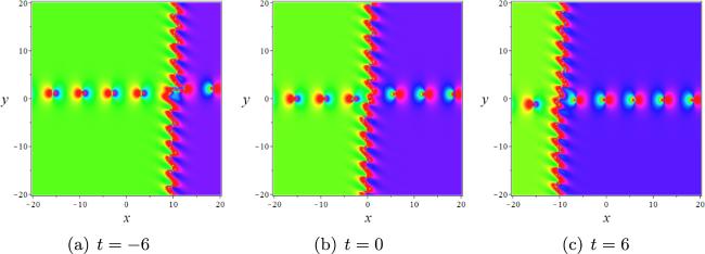
Figure 4. Second order breather solution to the 3D-eJM equation with ${p}_{1}^{}={p}_{2}^{* }=i$, ${p}_{3}^{}={p}_{4}^{* }=1+i$, ${q}_{1}^{}={q}_{2}^{* }=1$, ${q}_{3}^{}={q}_{4}^{* }=2i$, ${r}_{1}^{}={r}_{2}^{* }=2+i$, ${r}_{3}^{}={r}_{4}^{* }=2$, φ1 = φ2 = φ3 = φ4 = 0, z = 0 in equation ( |
The N-order lump solution also can be derivated from 2N-order soliton solution. As the procedure for finding the exact solution of lump using the long-wave limit method is well established, we directly provide following constraints:
$\begin{eqnarray}\begin{array}{ll} & {p}_{k}^{}={P}_{k}^{}\delta ,{q}_{k}^{}={Q}_{k}^{}\delta ,{r}_{k}^{}={R}_{k}^{}\delta ,\\ & {\omega }_{k}^{}={W}_{k}^{}\delta ,{{\rm{e}}}^{{\phi }_{k}}=-1,k=1,2,\cdots ,2N,\\ & {P}_{2s-1}^{}={P}_{2s}^{* },{Q}_{2s-1}^{}={Q}_{2s}^{* },\\ & {R}_{2s-1}^{}={R}_{2s}^{* },s=1,2,\cdots ,N.\end{array}\end{eqnarray}$
Then the N-order lump solution to the 3D-eJM equation can be acquired if we take δ → 0, specific forms are $\begin{eqnarray}\displaystyle \begin{array}{rcl}u & = & 2{\left(\mathrm{ln}{f}_{N}^{}\right)}_{x},\\ & & \quad k\lt s,p\lt q,m\lt n,p\lt \cdots \lt m,\\ {f}_{N}^{} & = & \prod _{k=1}^{2N}{\theta }_{k}^{}+{\sum }_{k,s}^{2N}\left({B}_{{ks}}^{}\displaystyle \prod _{j\ne k,s}^{2N}{\theta }_{j}^{}\right)\\ & & +\sum _{p,q,\cdots ,m,n}^{2N}\left({B}_{{pq}}^{}\cdots {B}_{{mn}}^{}\prod _{j\ne p,q,\cdots ,m,n}^{2N}{\theta }_{j}^{}\right)\cdots ,\end{array}\end{eqnarray}$
where $\begin{eqnarray}\begin{array}{rcl}{\theta }_{k}^{} & = & {P}_{k}^{}x+{Q}_{k}^{}y+{R}_{k}^{}z+{W}_{k}^{}t+{{\rm{\Phi }}}_{k},{W}_{k}^{}=\displaystyle \frac{3{R}_{k}^{}{P}_{k}^{}}{2({P}_{k}^{}+{Q}_{k}^{}+{R}_{k}^{})},\\ {B}_{{ks}} & = & \displaystyle \frac{2{P}_{k}^{}{P}_{s}^{}({P}_{k}^{}{Q}_{s}^{}+{P}_{s}^{}{Q}_{k}^{})({P}_{s}^{}+{Q}_{s}^{}+{R}_{s}^{})({P}_{k}^{}+{Q}_{k}^{}+{R}_{k}^{})}{\left[\left({Q}_{s}^{}+{R}_{s}^{}\right){P}_{k}^{}-\left({Q}_{k}^{}+{R}_{k}^{}\right){P}_{s}^{}\right]\left[\left({P}_{k}^{}+{Q}_{k}^{}\right){R}_{s}^{}-\left({P}_{s}^{}+{Q}_{s}^{}\right){P}_{k}^{}\right]},\end{array}\end{eqnarray}$
${P}_{k}^{},{Q}_{k}^{},{R}_{k}^{},{{\rm{\Phi }}}_{k}^{}$ are arbitrary constants, Φk affects the initial position of the corresponding lump solution. We usually study the trajectory of the wave crest of the lump wave. According to the solution of the system of equations $\left\{{u}_{x}=0,{u}_{y}=0\right\}$, we accquire the velocity formula of lump wave $\begin{eqnarray}\begin{array}{rcl}{V}_{\mathrm{lump}} & = & \left({V}_{x},{V}_{y}\right),\quad s=k+1\\ {V}_{x} & = & \displaystyle \frac{3{P}_{k}{P}_{s}({Q}_{k}{R}_{s}-{Q}_{s}{R}_{k})+3{P}_{s}{Q}_{k}{R}_{s}({Q}_{k}+{R}_{k})-3{P}_{k}{Q}_{s}{R}_{k}({Q}_{s}+{R}_{s})}{2({P}_{k}{Q}_{s}-{P}_{s}{Q}_{k})({P}_{k}+{Q}_{k}+{R}_{k})({P}_{s}+{Q}_{s}+{R}_{s})},\\ {V}_{y} & = & -\displaystyle \frac{3{P}_{k}{P}_{s}({P}_{k}{R}_{s}-{P}_{s}{R}_{k}+{Q}_{k}{R}_{s}-{Q}_{s}{R}_{k})}{2({P}_{k}{Q}_{s}-{P}_{s}{Q}_{k})({P}_{k}+{Q}_{k}+{R}_{k})({P}_{s}+{Q}_{s}+{R}_{s})},k=1,3,\cdots ,2N-1.\end{array}\end{eqnarray}$
When N = 1, with specific parameters, the expression of a first order lump wave is reduced as below: $\begin{eqnarray}\begin{array}{rcl}u & = & \displaystyle \frac{459014400x+573768000y+451008000t}{116640000{t}^{2}+225504000{xt}+195480000{yt}+114753600{x}^{2}+286884000{xy}+E},\\ E & = & 498062500{y}^{2}+571544649.\end{array}\end{eqnarray}$
We put the three-dimensional plot, density plot and sectional plot of the above solution in figure 5.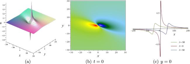
Figure 5. First order lump solution to the 3D-eJM equation with ${P}_{1}^{}={P}_{2}^{* }=0.2,{Q}_{1}^{}={Q}_{2}^{* }=\tfrac{1}{4}+\tfrac{1}{3}i$, ${R}_{1}^{}={R}_{2}^{* }=1$, Φ1 = Φ2 = 0, z = 0 in equation ( |
When N = 216 ). Second order lump solution can be represented by placing equation (19 ) in equation (3 ) as shown in figure 6. We make ${\phi }_{k}^{}\left(k=1,2,3,4\right)$ not all zero, allowing us to split the trajectory of the two first order lump solutions. Their speeds are $\left(-\tfrac{9180}{7969},\tfrac{1080}{7969}\right),\left(-\tfrac{31110}{37283},-\tfrac{18750}{37283}\right)$ respectively.
$\begin{eqnarray}\begin{array}{rcl}f & = & {\theta }_{1}{\theta }_{2}{\theta }_{3}{\theta }_{4}+{B}_{12}{\theta }_{3}{\theta }_{4}+{B}_{13}{\theta }_{2}{\theta }_{4}\\ & & +{B}_{14}{\theta }_{2}{\theta }_{3}+{B}_{23}{\theta }_{1}{\theta }_{4}+{B}_{24}{\theta }_{1}{\theta }_{3}\\ & & +{B}_{34}{\theta }_{1}{\theta }_{2}+{B}_{12}{B}_{34}\\ & & +{B}_{13}{B}_{24}+{B}_{14}{B}_{23},\end{array}\end{eqnarray}$
where ${\theta }_{k}^{},{B}_{{ks}}^{}$ meet the equation (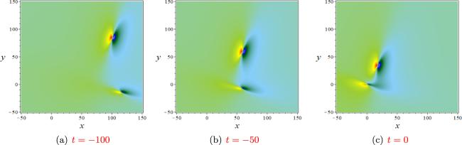
Figure 6. Second order lump solution to the 3D-eJM equation with ${P}_{1}^{}={P}_{2}^{* }=0.2,{P}_{3}^{}={P}_{4}^{* }=0.75+i$, ${Q}_{1}^{}={Q}_{2}^{* }=\tfrac{1}{4}+\tfrac{1}{3}i$, ${Q}_{3}^{}={Q}_{4}^{* }\,=0.2-0.5i$, ${R}_{1}^{}={R}_{2}^{* }={R}_{3}^{}={R}_{4}^{* }=1$, Φ1 = Φ2 = 0, Φ3 = Φ4 = −20, z = 0 in equation ( |
As we all know that two soliton will transform to resonance Y-type soliton if we take suitable ${p}_{i}^{},{q}_{i}^{},{r}_{i}^{}(i=1,2)$ in accordance with $\exp ({A}_{{ks}})=0$ and $\left\{{p}_{k}^{}\ne {p}_{s}^{}\ \mathrm{or}\ {q}_{k}^{}\ne {q}_{s}^{}\ \mathrm{or}\ {r}_{k}^{}\ne {r}_{s}^{}\right\}$. The speed of Y-type structure solution has rarely been investigated in the previous literature. We likewise provide an expression for its velocity by analysing the variation with time of the position of the intersection point,
$\begin{eqnarray}\begin{array}{l}{V}_{{\rm{Y}}-{\mathrm{type}}^{}}=\left({V}_{x},{V}_{y}\right)\\ =\,\left(-\displaystyle \frac{{\omega }_{k}^{}{q}_{s}^{}-{\omega }_{s}^{}{q}_{k}^{}}{{p}_{k}^{}{q}_{s}^{}-{p}_{s}^{}{q}_{k}^{}},\displaystyle \frac{{\omega }_{k}^{}{p}_{s}^{}-{\omega }_{s}^{}{p}_{k}^{}}{{p}_{k}^{}{q}_{s}^{}-{p}_{s}^{}{q}_{k}^{}}\right),\\ {\omega }_{k}^{}=-\displaystyle \frac{{p}_{k}^{3}{q}_{k}^{}-3{p}_{k}^{}{r}_{k}^{}}{2({p}_{k}^{}+{q}_{k}^{}+{r}_{k}^{})}.\end{array}\end{eqnarray}$
Let N = 2, the f is transformed to 2-resonance Y-type solution as7 ), and this phenomenon can be observed in figure 7. The velocity of above solution is $\left(\tfrac{14+7\sqrt{247}}{100-4\sqrt{247}},\tfrac{153+9\sqrt{247}}{-200+8\sqrt{247}}\right)$.
$\begin{eqnarray}f=1+{{\rm{e}}}^{{\xi }_{1}}+{{\rm{e}}}^{{\xi }_{2}},\end{eqnarray}$
where ξk are given by equation (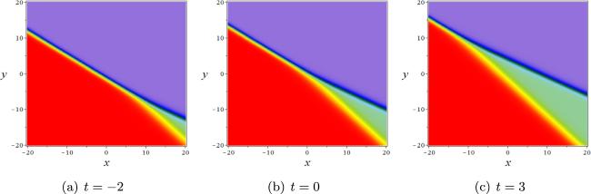
Figure 7. 2-resonance Y-type solution to the 3D-eJM equation with p1 = 1, q1 = 1, r1 = 2, p2 = 2, q2 = 3, ${r}_{2}=\tfrac{65}{7}-\tfrac{4\sqrt{247}}{7}$, φ1 = φ2 = 0, z = 0 in equation ( |
Let N = 3, with $\exp ({A}_{12})=\exp ({A}_{13})=0$, the f is reduced as7 ) and equation (13 ). Substitute equation (22 ) in equation (3 ), we achieve two different kinds of 3-resonance Y-type solutions as show in figure 8. One in x − y and z = 0 plane, the other is in y − z and x = 0 plane. The shape of solution in figure 8(a) is similar to that of X.
$\begin{eqnarray}f=1+{{\rm{e}}}^{{\xi }_{1}}+{{\rm{e}}}^{{\xi }_{2}}+{{\rm{e}}}^{{\xi }_{3}}+{b}_{23}{{\rm{e}}}^{{\xi }_{2}+{\xi }_{3}},\end{eqnarray}$
where ξk, bks are given by equation (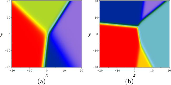
Figure 8. Two kinds of 3-resonance Y-type solutions to the 3D-eJM equation with (a): p1 = 1, q1 = 1, r1 = 2, p2 = 2 , ${q}_{2}=1-\tfrac{4\sqrt{11}}{11},{r}_{2}=1,{p}_{3}=\tfrac{1}{2}$ , ${q}_{3}=\tfrac{4}{9}-\tfrac{\sqrt{7}}{18},{r}_{3}=\tfrac{1}{3}$, φ1 = φ2 = φ3 = 0, z = 0; (b): p1 = 1, q1 = 1, r1 = 2, p2 = 2 , ${q}_{2}=3,{r}_{2}=\tfrac{65}{7}-\tfrac{4\sqrt{247}}{7},{p}_{3}=-\tfrac{1}{2}$, ${q}_{3}=\tfrac{1}{3},{r}_{3}=-\tfrac{101}{84}-\tfrac{\sqrt{9865}}{84},{\phi }_{1}=0$, φ2 = − 10, φ3 = 10, x = 0 in equation ( |
3. Molecules composed of the same waves
In the last section we focused on four types of local waves and gave expressions for their respective velocities. It is not hard to see from the images of the higher-order solutions that a higher-order solution can be seen as an interaction phenomenon between several lower-order solutions. Much literature shows that collisions between these four local waves are all elastic collisions, the same as between two line waves [44-46]. It is well known that assuming that the velocities of the two lower order solutions are identical (including the x, y axes), the two solutions are bound into a new structure during the motion called molecule solution. This section demonstrates several molecule solutions consisting of the same local wave.
To investigate the single line molecule solution, the fuction f can be choosed as same as second order soliton solution. With the parameters as the figures 9(a)-(c), the u can be unfolded as23 ) is $\left(\tfrac{1128-132\sqrt{151}}{629},\tfrac{237\sqrt{151}-2883}{629}\right)$. In fact, the equation contains special molecule solutions which is obtained as long as $\{{p}_{1}^{2}{q}_{1}^{}-3{r}_{1}={p}_{2}^{2}{q}_{2}^{}-3{r}_{2}^{}=0\}$, while the selecting parameters $\tfrac{{p}_{1}}{{p}_{2}}=\tfrac{{q}_{1}}{{q}_{2}}=\tfrac{{\omega }_{1}}{{\omega }_{2}}$ and arbitrary ${r}_{1}^{},{r}_{2}^{}$ gives the equation (23 ).
$\begin{eqnarray}\begin{array}{rcl}{u}_{2}^{} & = & \displaystyle \frac{8\left(\exp \left({\varphi }_{1}\right)+3\ \exp \left({\varphi }_{2}\right)+\exp \left({\varphi }_{3}\right)\right)}{\left(4\ \exp \left({\varphi }_{1}\right)+4\ \exp \left({\varphi }_{2}\right)+\exp \left({\varphi }_{3}\right)+4\right)},\\ {\varphi }_{1} & = & \displaystyle \frac{(6x-y-3t-30)\sqrt{151}+66x+4y+147t-330}{66+6\sqrt{151}},\\ {\varphi }_{2} & = & \displaystyle \frac{(6x-3y-27t+10)\sqrt{151}+42x+30y+423t+70}{14+2\sqrt{151}},\\ {\varphi }_{3} & = & \displaystyle \frac{(42t+36x-y)\sqrt{151}+192t+456x-41y}{114+9\sqrt{151}}.\end{array}\end{eqnarray}$
While solutions satisfy the definition of molecule solution: bound into one and not changing relative position, the velocity of solution (
Figure 9. Single line molecule solutions to the 3D-eJM equation with p1 = 1, p2 = 3, r1 = 1, r2 = 2, ${q}_{1}=-\tfrac{13}{12}+\tfrac{\sqrt{151}}{12},{q}_{2}=-\tfrac{13}{4}+\tfrac{\sqrt{151}}{4},{\phi }_{1}=-5,{\phi }_{2}=5,z=0$ in equation ( |
If we take f as same as equation (13 ), the interaction solution between two line molecule solutions is showed in figure 10. Their velocities are $\left(\tfrac{1128+132\sqrt{151}}{629},-\tfrac{2883+237\sqrt{151}}{629}\right)$, $\left(\tfrac{93-5\sqrt{1329}}{104},\tfrac{9\sqrt{1329}-321}{104}\right)$ respectively.

Figure 10. Interaction solution between two line molecule solutions with p1 = 1, p2 = 3, r1 = 1, r2 = 2, ${q}_{1}=-\tfrac{13}{12}-\tfrac{\sqrt{151}}{12},{q}_{2}=-\tfrac{13}{4}-\tfrac{\sqrt{151}}{4}$, ${p}_{3}=2,{p}_{4}=4,{r}_{3}=2,{r}_{4}=1,{q}_{3}=-\tfrac{39}{16}+\tfrac{\sqrt{1329}}{16}$ , ${q}_{4}=-\tfrac{39}{8}+\tfrac{\sqrt{1329}}{8},{\phi }_{1}=-15,{\phi }_{2}=-10,{\phi }_{3}=0,{\phi }_{4}=8,z=0$ in equation ( |
In particular, we find the velocity resonance among two breather waves by picking parameters in equation (13 ) meet module resonance condition and
$\begin{eqnarray}\begin{array}{l}\left(-\displaystyle \frac{{\mathfrak{R}}({\omega }_{1}^{}){\mathfrak{R}}({p}_{1}^{})}{{\mathfrak{R}}{\left({p}_{1}^{}\right)}^{2}+{\mathfrak{R}}{\left({q}_{1}^{}\right)}^{2}},-\displaystyle \frac{{\mathfrak{R}}({\omega }_{1}^{}){\mathfrak{R}}({q}_{1}^{})}{{\mathfrak{R}}{\left({p}_{1}^{}\right)}^{2}+{\mathfrak{R}}{\left({q}_{1}^{}\right)}^{2}}\right)\\ =\left(-\displaystyle \frac{{\mathfrak{R}}({\omega }_{3}^{}){\mathfrak{R}}({p}_{3}^{})}{{\mathfrak{R}}{\left({p}_{3}^{}\right)}^{2}+{\mathfrak{R}}{\left({q}_{3}^{}\right)}^{2}},-\displaystyle \frac{{\mathfrak{R}}({\omega }_{3}^{}){\mathfrak{R}}({q}_{3}^{})}{{\mathfrak{R}}{\left({p}_{3}^{}\right)}^{2}+{\mathfrak{R}}{\left({q}_{3}^{}\right)}^{2}}\right),\end{array}\end{eqnarray}$
i.e. $\tfrac{{\mathfrak{R}}({p}_{1}^{})}{{\mathfrak{R}}({p}_{2}^{})}=\tfrac{{\mathfrak{R}}({q}_{1}^{})}{{\mathfrak{R}}({q}_{2}^{})}=\tfrac{{\mathfrak{R}}({\omega }_{1}^{})}{{\mathfrak{R}}({\omega }_{2}^{})}$. The breather molecule solution is vividly represented in figure 11 and the expression is expanded as $\begin{eqnarray}\begin{array}{rcl}f & = & 1+\exp \left(2y+\displaystyle \frac{5t}{13}-10\right)\\ & & -\displaystyle \frac{208472563}{20177273}\exp \left(6y+\displaystyle \frac{15t}{13}+6\right)\\ & & -\displaystyle \frac{151}{5}\exp \left(4y+\displaystyle \frac{10t}{13}+16\right)\\ & & +2\ \exp \left(y+\displaystyle \frac{5t}{26}-5\right)\cos \left(x+\displaystyle \frac{27t}{26}\right)\\ & & +2\ \exp \left(y+\displaystyle \frac{5t}{13}+8\right)\cos \left(x+\displaystyle \frac{27t}{26}\right)\\ & & +\exp \left(3y+\displaystyle \frac{15t}{26}+3\right)\left[\displaystyle \frac{90418}{276401}\cos \left(3x+4y+\displaystyle \frac{105t}{26}\right)\right.\\ & & +\displaystyle \frac{290}{73}\cos \left(x+4y+\displaystyle \frac{49t}{26}\right)\\ & & -\displaystyle \frac{38064}{276401}\sin \left(3x+4y+\displaystyle \frac{105t}{26}\right)\\ & & \left.+\displaystyle \frac{384}{73}\sin \left(x+4y+\displaystyle \frac{49t}{26}\right)\right]\\ & & +\exp \left(4y+\displaystyle \frac{10t}{13}-2\right)\left[\displaystyle \frac{5802322}{20177273}\cos \left(2x+4y+\displaystyle \frac{38t}{13}\right)\right.\\ & & \left.-\displaystyle \frac{22879536}{20177273}\sin \left(\displaystyle \frac{38t}{13}+4y+2x\right)\right]\\ & & -\exp \left(5y+\displaystyle \frac{25t}{26}+11\right)\left[\displaystyle \frac{3083253598}{100886365}\cos \left(x+\displaystyle \frac{27t}{26}\right)\right.\\ & & \left.+\displaystyle \frac{1787987376}{100886365}\sin \left(x+\displaystyle \frac{27t}{26}\right)\right].\end{array}\end{eqnarray}$

Figure 11. Single breather molecule solution to the 3D-eJM equation with ${p}_{1}^{}={p}_{2}^{* }=i,{q}_{1}^{}={q}_{2}^{* }=1$, ${r}_{1}^{}={r}_{2}^{* }=2+i,{p}_{3}^{}={p}_{4}^{* }=2i,{r}_{3}^{}={r}_{4}^{* }=2$ , ${q}_{3}^{}={q}_{4}^{* }=2+4i,{\phi }_{1}={\phi }_{2}=-5,{\phi }_{3}={\phi }_{4}=8,z=0$ in equation ( |
Based the bilinear form, like the lump molecule solution which does not exist in many (2+1)-dimensional integrable models, such as the (2+1)-dimensional generalized Bogoyavlensky-Konopelchenko model [38], Kadomtsev-Petviashvili (KP) system [39], (3+1)-dimensional nagative order KdV-CBS model [47], etc. But for KP systerm, lump molecules can be discovered by using the reduced version of the Grammian form [35, 40]. With the aid of equation (17 ), we find the lump molecule solution in equation (2 ), which needs to cater for19 ). figure 12 vividly depicts this type of molecule solution with speed $\left(-\tfrac{21}{25},\tfrac{3}{25}\right)$, the distance between the centres of two single lump solution is constant.
$\begin{eqnarray}\begin{array}{rcl} & & \displaystyle \frac{3{P}_{1}{P}_{2}({Q}_{1}{R}_{2}-{Q}_{2}{R}_{1})+3{P}_{2}{Q}_{1}{R}_{2}({Q}_{1}+{R}_{1})-3{P}_{1}{Q}_{2}{R}_{1}({Q}_{2}+{R}_{2})}{2({P}_{1}{Q}_{2}-{P}_{2}{Q}_{1})({P}_{1}+{Q}_{1}+{R}_{1})({P}_{2}+{Q}_{2}+{R}_{2})}\\ & = & \displaystyle \frac{3{P}_{3}{P}_{4}({Q}_{3}{R}_{4}-{Q}_{4}{R}_{3})+3{P}_{4}{Q}_{3}{R}_{4}({Q}_{3}+{R}_{3})-3{P}_{3}{Q}_{4}{R}_{3}({Q}_{4}+{R}_{4})}{2({P}_{3}{Q}_{4}-{P}_{4}{Q}_{3})({P}_{3}+{Q}_{3}+{R}_{3})({P}_{4}+{Q}_{4}+{R}_{4})},\\ & & \displaystyle \frac{({P}_{3}{Q}_{4}-{P}_{4}{Q}_{3})({P}_{3}+{Q}_{3}+{R}_{3})({P}_{4}+{Q}_{4}+{R}_{4})}{({P}_{1}{Q}_{2}-{P}_{2}{Q}_{1})({P}_{1}+{Q}_{1}+{R}_{1})({P}_{2}+{Q}_{2}+{R}_{2})}=\displaystyle \frac{{P}_{3}{P}_{4}({P}_{3}{R}_{4}-{P}_{4}{R}_{3}+{Q}_{3}{R}_{4}-{Q}_{4}{R}_{3})}{{P}_{1}{P}_{2}({P}_{1}{R}_{2}-{P}_{2}{R}_{1}+{Q}_{1}{R}_{2}-{Q}_{2}{R}_{1})},\\ & & {P}_{1}^{}={P}_{2}^{* },{P}_{3}^{}={P}_{4}^{* },{Q}_{1}^{}={Q}_{2}^{* },{Q}_{3}^{}={Q}_{4}^{* },{R}_{1}^{}={R}_{2}^{* },{R}_{3}^{}={R}_{4}^{* }\end{array}\end{eqnarray}$
in equation (
Figure 12. Single lump molecule solution to the 3D-eJM equation with ${P}_{1}={P}_{2}^{* }=1+\tfrac{1}{2}i$, ${Q}_{1}={Q}_{2}^{* }=\tfrac{1}{2}-i$, ${R}_{1}={R}_{2}^{* }=2,{P}_{3}$ = ${P}_{4}^{* }=\tfrac{11}{28}-\tfrac{\sqrt{-1806+10\sqrt{36313}}}{56}$ + $\left(-\tfrac{6}{7}+\tfrac{(903+5\sqrt{36313})\sqrt{-1806\,+\,10\sqrt{36313}}}{17024}\right)i$, ${Q}_{3}={Q}_{4}^{* }=2i$, ${R}_{3}={R}_{4}^{* }=1$, Φ1 = Φ2 = 0, Φ3 = Φ4 = 300, z = 0 in equation ( |
4. Molecules made up of the different waves
In this section, we investigate molecule solutions consisting of different localized waves. It is obvious from the previous analysis that, again, no contact occurs between waves, which remain relatively stationary. The function f can be chosen as7 ) and (13 ). Like the one shown in the figure 13, the line wave move parallel to the breather with the same speed $\left(-\tfrac{129}{740},\tfrac{129}{370}\right)$. Once the coefficients of x, y, z, t have been determined, φ1, φ3 determines the distance between the two solutions. By φ1 = φ3, we find a phenomenon shown in figure 14, the breather collides line wave continuously and changes its own form.
$\begin{eqnarray}\begin{array}{l}f=1+{{\rm{e}}}^{{\xi }_{1}}+{{\rm{e}}}^{{\xi }_{2}}+{{\rm{e}}}^{{\xi }_{3}}\\ +{b}_{12}^{}{{\rm{e}}}^{{\xi }_{1}+{\xi }_{2}}+{b}_{13}^{}{{\rm{e}}}^{{\xi }_{1}+{\xi }_{3}}\\ +{b}_{23}^{}{{\rm{e}}}^{{\xi }_{2}+{\xi }_{3}}+{b}_{12}^{}{b}_{13}^{}{b}_{23}^{}{{\rm{e}}}^{{\xi }_{1}+{\xi }_{2}+{\xi }_{3}},\end{array}\end{eqnarray}$
if we want to look for the line-breather molecule which consisting of a single line and a single wave. ξk, bks are given by equation (
Figure 13. Line-breather molecule with ${p}_{1}=\tfrac{1}{2}+i$, ${q}_{1}=-1,{r}_{1}=\tfrac{1}{3}$, ${p}_{2}=\tfrac{1}{2}-i$, ${q}_{2}=-1,{r}_{2}=\tfrac{1}{3}$, p3 = 1, q3 = − 2, ${r}_{3}=-\tfrac{277}{93}$, φ1 = φ2 = 0, φ3 = 10, z = 0 in equation ( |

Figure 14. Always collide case with φ1 = φ2 = φ3 = 0, other parameters are consistent with figure 13. |
When searching for a molecule solution consisting of lump solution and other solutions, the partial long-wave limit method is required. For example, let7 ), (16 ) and
$\begin{eqnarray}\begin{array}{ll} & N=3,{p}_{k}^{}={P}_{k}^{}\delta ,\\ & {q}_{k}^{}={Q}_{k}^{}\delta ,{r}_{k}^{}={R}_{k}^{}\delta ,{\phi }_{k}=i\pi ,\\ & {P}_{1}={P}_{2}^{* },{Q}_{1}={Q}_{2}^{* },\\ & {R}_{1}={R}_{2}^{* },\delta \to 0,k=1,2,\end{array}\end{eqnarray}$
then the lump-line molecule solution can be reflected by following formula $\begin{eqnarray}\begin{array}{rcl}u & = & 2{\left(\mathrm{ln}f\right)}_{x},\\ f & = & {\theta }_{1}{\theta }_{2}+{B}_{12}+{e}^{{\xi }_{3}}({\theta }_{1}{\theta }_{2}+{B}_{12}\\ & & +{B}_{13}{B}_{23}+{B}_{23}{\theta }_{1}+{B}_{13}{\theta }_{2}),\end{array}\end{eqnarray}$
$\begin{eqnarray}\begin{array}{cc} & {B}_{{ks}}=\left\{\begin{array}{c}\displaystyle \frac{\left.2{P}_{k}^{}{P}_{s}^{}({P}_{k}^{}{Q}_{s}^{}+{P}_{s}^{}{Q}_{k}^{})({P}_{s}^{}+{Q}_{s}^{}+{R}_{s}^{})({P}_{k}^{}+{Q}_{k}^{}+{R}_{k}^{}\right)}{\left[\left({Q}_{s}^{}+{R}_{s}^{}\right){P}_{k}^{}-\left({Q}_{k}^{}+{R}_{k}^{}\right){P}_{s}^{}\right]\left[\left({P}_{k}^{}+{Q}_{k}^{}\right){R}_{s}^{}-\left({P}_{s}^{}+{Q}_{s}^{}\right){P}_{k}^{}\right]}k,s\lt 3,\\ \\ -\displaystyle \frac{\left.6{P}_{k}{p}_{s}({p}_{s}+{q}_{s}+{r}_{s})({q}_{s}{P}_{k}+{Q}_{k}{p}_{s})({Q}_{k}+{P}_{k}+{R}_{k}\right)}{{p}_{s}^{s}({Q}_{k}+{P}_{k}+{R}_{k})({p}_{s}{Q}_{k}+2{q}_{s}{P}_{k}+{r}_{s}{Q}_{k}-{R}_{k}{q}_{s})+Z},\,k\lt 3,s\geqslant 3,\end{array}\right.\\ & Z=3{p}_{s}^{2}\left({P}_{k}{q}_{s}\left({q}_{s}+{r}_{s})({Q}_{k}+{P}_{k}+{R}_{k})-{R}_{k}({Q}_{k}+{R}_{k}\right)\right)\\ & \,\,+3{p}_{s}\left(\left({r}_{s}{Q}_{k}+{R}_{k}{q}_{s}+2{r}_{s}{R}_{k}){P}_{k}+({Q}_{k}+{R}_{k})({r}_{s}{Q}_{k}-{R}_{k}{q}_{s}\right)\right)\\ & \,\,-3{P}_{k}({q}_{s}+{r}_{s})({P}_{k}{r}_{s}+{r}_{s}{Q}_{k}-{R}_{k}{q}_{s}).\end{array}\end{eqnarray}$
where ξ3, θ1, θ2 suit equation ( $\begin{eqnarray}\begin{array}{ll} & \displaystyle \frac{((3{Q}_{1}{R}_{2}-3{Q}_{2}{R}_{1}){P}_{2}-3{Q}_{2}{R}_{1}({Q}_{2}+{R}_{2})){P}_{1}+3{P}_{2}{Q}_{1}{R}_{2}({Q}_{1}+{R}_{1})}{2({P}_{2}+{Q}_{2}+{R}_{2})({P}_{1}{Q}_{2}-{P}_{2}{Q}_{1})({P}_{1}+{Q}_{1}+{R}_{1})}\\ & =\displaystyle \frac{{p}_{3}^{2}({p}_{3}^{2}{q}_{3}-3{r}_{3})}{2({p}_{3}+{q}_{3}+{r}_{3})({p}_{3}^{2}+{q}_{3}^{2})},-\displaystyle \frac{3{P}_{1}{P}_{2}({P}_{1}{R}_{2}-{P}_{2}{R}_{1}+{Q}_{1}{R}_{2}-{Q}_{2}{R}_{1})}{2({P}_{2}+{Q}_{2}+{R}_{2})({P}_{1}{Q}_{2}-{P}_{2}{Q}_{1})({P}_{1}+{Q}_{1}+{R}_{1})}\\ & =\displaystyle \frac{{p}_{3}{q}_{3}({p}_{3}^{2}{q}_{3}-3{r}_{3})}{2({p}_{3}+2{q}_{3}+{r}_{3})({p}_{3}^{2}+{q}_{3}^{2})},\end{array}\end{eqnarray}$
When the coefficients of x, y, z, t satisfiesthe lump-line solution will be located on figure 15 with velocity $\left(-\tfrac{8298}{11237},-\tfrac{4050}{11237}\right)$.
Figure 15. Lump-line molecule solution with ${P}_{1}={P}_{2}^{* }=\tfrac{3}{4}+i$, ${Q}_{1}={Q}_{2}^{* }=\tfrac{1}{3}-\tfrac{1}{2}i$, ${R}_{1}={R}_{2}^{* }=1$, p3 = 1 , ${q}_{3}=\tfrac{225}{461}$ , ${r}_{3}=\tfrac{2554737147}{932374805}$, Φ1 = Φ2 = 0, φ3 = 35, z = 0 in equation ( |
When adjusting φ3 to 0, the line wave passes exactly through the centre of the lump solution and the two waves merge to form a lump-kink solution. And the lump solution is divided into exactly two section, with the upwardly raised part on top of the kinked area and vice versa. The method used for the idea just mentioned is different from the test function method which test function f is
$\begin{eqnarray}\begin{array}{rcl}f & = & {\left({a}_{1}x+{a}_{2}y+{a}_{3}z+{a}_{4}t+{a}_{5}\right)}^{2}\\ & & +{\left({b}_{1}x+{b}_{2}y+{b}_{3}z+{b}_{4}t+{b}_{5}\right)}^{2}\\ & & +\exp \left({c}_{1}x+{c}_{2}y+{c}_{3}z+{c}_{4}t+{c}_{5}\right)+k.\end{array}\end{eqnarray}$
The method we use has the advantage that the excitation method is more stable and does not change over time. This interesting situation is shown in figure 16 with expression $\begin{eqnarray}\begin{array}{rcl}u & = & 2{\left(\mathrm{ln}f\right)}_{x},\\ f & = & \left(\displaystyle \frac{2025}{2644}{t}^{2}+\displaystyle \frac{5625}{2644}{xt}-\displaystyle \frac{72}{661}{yt}-\displaystyle \frac{12138571156418651344144725}{5528705278408403241790792}t+\displaystyle \frac{25}{16}{x}^{2}-\displaystyle \frac{1}{2}{xy}\right.\\ & & -\displaystyle \frac{45237306482980701003580875}{11057410556816806483581584}x+\displaystyle \frac{13}{36}{y}^{2}+\displaystyle \frac{12663817410669269953013031}{5528705278408403241790792}y\\ & & \left.+\displaystyle \frac{37325014127412831248801817275}{5440245993953868789922139328}\right)\exp \left(x+\displaystyle \frac{225y}{461}+\displaystyle \frac{4736628t}{5180257}\right)+\displaystyle \frac{2025{t}^{2}}{2644}\\ & & +\displaystyle \frac{5625}{2644}{xt}-\displaystyle \frac{72}{661}{yt}+\displaystyle \frac{25{x}^{2}}{16}-\displaystyle \frac{{xy}}{2}+\displaystyle \frac{13{y}^{2}}{36}+\displaystyle \frac{16525}{7872}.\end{array}\end{eqnarray}$

Figure 16. Lump-kink solution to the 3D-eJM equation with Φ3 = 0, other parameters are consistent with figure 15. |
We promote on the basis of equation (28 ) that7 ), (13 ) and (30 ). On this basis we find two different scenarios. The first case is where the lump solution forms a bound molecule with one of the line waves and moves in the direction in which the other line wave is located. The distance between the lump solution and the two line waves remains fixed, although there is a change in relative position between the two line waves as time changes, and this can be interpreted as a lump-2 line solution in the weak sense. Another case is that the lump solution and the two line waves as a whole form a molecule solution, i.e. lump-2 line solution. These two cases are shown in figures 17 and 18. The velocity of the molecule solution in both diagrams is $\left(-\tfrac{21}{34},\tfrac{39}{340}\right)$, and other line wave is $\left(0,0\right)$.
$\begin{eqnarray}\begin{array}{ll} & N=4,{p}_{k}^{}={P}_{k}^{}\delta ,{q}_{k}^{}={Q}_{k}^{}\delta ,\\ & {r}_{k}^{}={R}_{k}^{}\delta ,{\phi }_{k}={\rm{i}}\pi ,\\ & {P}_{1}={P}_{2}^{* },{Q}_{1}={Q}_{2}^{* },\\ & {R}_{1}={R}_{2}^{* },\delta \to 0,k=1,2,\end{array}\end{eqnarray}$
then the interaction solution between lump and two line waves is derived from $\begin{eqnarray}u=2{\left(\mathrm{ln}f\right)}_{x},\end{eqnarray}$
and $\begin{eqnarray}\begin{array}{rcl}f & = & {{\rm{e}}}^{{\xi }_{3}}({\theta }_{1}{\theta }_{2}+{B}_{12}+{B}_{13}{B}_{23}+{B}_{23}{\theta }_{1}+{B}_{13}{\theta }_{2})\\ & & +{{\rm{e}}}^{{\xi }_{4}}({\theta }_{1}{\theta }_{2}+{B}_{12}+{B}_{14}{B}_{24}+{B}_{24}{\theta }_{1}+{B}_{14}{\theta }_{2})\\ & & +{b}_{34}{{\rm{e}}}^{{\xi }_{3}+{\xi }_{4}}({\theta }_{1}{\theta }_{2}+{B}_{12}+{B}_{23}{\theta }_{1}\\ & & +{B}_{24}{\theta }_{1}+{B}_{13}{\theta }_{2}+{B}_{14}{\theta }_{2}+{B}_{13}{B}_{23}\\ & & +{B}_{13}{B}_{24}+{B}_{14}{B}_{23}+{B}_{14}{B}_{24})+{\theta }_{1}{\theta }_{2}+{B}_{12},\end{array}\end{eqnarray}$
where ξk, θk, Bks, b34 suit equations (
Figure 17. Lump-line molecule solution with ${P}_{1}={P}_{2}^{* }=\tfrac{3}{4}+\tfrac{1}{2}{\rm{i}}$, ${Q}_{1}={Q}_{2}^{* }=\tfrac{1}{2}-{\rm{i}}$, ${R}_{1}={R}_{2}^{* }=1$, ${p}_{3}=2,{q}_{3}=-\tfrac{13}{35}$, ${r}_{3}=\tfrac{247999}{717255}$, ${p}_{4}=\tfrac{13}{6}$, ${q}_{4}=\tfrac{70}{6}$, ${r}_{4}=\tfrac{5915}{324}$, Φ1 = Φ2 = 0, φ3 = 5, φ4 = 50, z = 0 in equation ( |

Figure 18. The first case of equation ( |
Since the 2-resonance Y-type solution is derived from the two-soliton solution and we have given lump-2 line molecule in figure 17, it follows that molecule solution consisting of lump solution and 2-resonance Y-type solution must exist in this system. If equation (35 ) meet the following parameter restrictions
$\begin{eqnarray}\begin{array}{ll} & \displaystyle \frac{((3{Q}_{1}{R}_{2}-3{Q}_{2}{R}_{1}){P}_{2}-3{Q}_{2}{R}_{1}({Q}_{2}+{R}_{2})){P}_{1}+3{P}_{2}{Q}_{1}{R}_{2}({Q}_{1}+{R}_{1})}{2({P}_{2}+{Q}_{2}+{R}_{2})({P}_{1}{Q}_{2}-{P}_{2}{Q}_{1})({P}_{1}+{Q}_{1}+{R}_{1})}=-\displaystyle \frac{{\omega }_{3}^{}{q}_{4}^{}-{\omega }_{4}^{}{q}_{3}^{}}{{p}_{3}^{}{q}_{4}^{}-{p}_{4}^{}{q}_{3}^{}},\\ & -\displaystyle \frac{3{P}_{1}{P}_{2}({P}_{1}{R}_{2}-{P}_{2}{R}_{1}+{Q}_{1}{R}_{2}-{Q}_{2}{R}_{1})}{2({P}_{2}+{Q}_{2}+{R}_{2})({P}_{1}{Q}_{2}-{P}_{2}{Q}_{1})({P}_{1}+{Q}_{1}+{R}_{1})}=\displaystyle \frac{{\omega }_{3}^{}{p}_{4}^{}-{\omega }_{4}^{}{p}_{3}^{}}{{p}_{3}^{}{q}_{4}^{}-{p}_{4}^{}{q}_{3}^{}},\quad {B}_{34}=0,\\ & {\omega }_{k}^{}=-\displaystyle \frac{{p}_{k}^{3}{q}_{k}^{}-3{p}_{k}^{}{r}_{k}^{}}{2({p}_{k}^{}+{q}_{k}^{}+{r}_{k}^{})},\end{array}\end{eqnarray}$
then it can be denoted as lump-resonance Y-type molecule solution in figure 19. Lump solution is located in the middle of the two branches of the resonance Y-type solution, and the distance between the lump solution and the two branches remains the same from the beginning to the end. This molecule solution is moving at $\left(\tfrac{49}{136},-\tfrac{33}{136}\right)$.
Figure 19. Lump-resonance Y-type molecule solution to the 3D-eJM equation with ${P}_{1}={P}_{2}^{* }=1+\tfrac{1}{2}{\rm{i}}$, ${Q}_{1}={Q}_{2}^{* }$ = $\left(-\tfrac{49}{66}+\tfrac{\left(-\sqrt{194021545}+13104\right)\sqrt{13104+\sqrt{194021545}}}{311718}\right)$ + $\left(\tfrac{8}{66}-\tfrac{\sqrt{13104+\sqrt{194021545}}}{66}\right){\rm{i}}$, ${R}_{1}={R}_{2}^{* }=1$, p3 = 1, q3 = 2, r3 = 1, p4 = −2, ${q}_{4}=\tfrac{24}{11}$ , r4 = 2, Φ1 = Φ2 = 0, φ3 = φ4 = −40, z = 0 in equation ( |
If equation (36 ) meet the module resonance condition and12 ), then the lump-breather solution is vividly described in figure 20 with $\left(-\tfrac{2}{5},\tfrac{4}{5}\right)$.
$\begin{eqnarray}\begin{array}{ll} & -\displaystyle \frac{{\mathfrak{R}}({\omega }_{3}^{}){\mathfrak{R}}({p}_{3}^{})}{{\mathfrak{R}}{\left({p}_{3}^{}\right)}^{2}+{\mathfrak{R}}{\left({q}_{3}^{}\right)}^{2}}=\displaystyle \frac{((3{Q}_{1}{R}_{2}-3{Q}_{2}{R}_{1}){P}_{2}-3{Q}_{2}{R}_{1}({Q}_{2}+{R}_{2})){P}_{1}+3{P}_{2}{Q}_{1}{R}_{2}({Q}_{1}+{R}_{1})}{2({P}_{2}+{Q}_{2}+{R}_{2})({P}_{1}{Q}_{2}-{P}_{2}{Q}_{1})({P}_{1}+{Q}_{1}+{R}_{1})},\\ & -\displaystyle \frac{{\mathfrak{R}}({\omega }_{3}^{}){\mathfrak{R}}({q}_{3}^{})}{{\mathfrak{R}}{\left({p}_{3}^{}\right)}^{2}+{\mathfrak{R}}{\left({q}_{3}^{}\right)}^{2}}=-\displaystyle \frac{3{P}_{1}{P}_{2}({P}_{1}{R}_{2}-{P}_{2}{R}_{1}+{Q}_{1}{R}_{2}-{Q}_{2}{R}_{1})}{2({P}_{2}+{Q}_{2}+{R}_{2})({P}_{1}{Q}_{2}-{P}_{2}{Q}_{1})({P}_{1}+{Q}_{1}+{R}_{1})},\end{array}\end{eqnarray}$
where ω3 is given by equation (
Figure 20. Lump-breather molecule solution to the 3D-eJM equation with ${P}_{1}={P}_{2}^{* }=1+\tfrac{1}{2}{\rm{i}}$, ${Q}_{1}={Q}_{2}^{* }=-\tfrac{3}{4}+\tfrac{\sqrt{29}-1}{8}{\rm{i}}$, ${R}_{1}={R}_{2}^{* }=1$, ${p}_{3}={p}_{4}^{* }=1+{\rm{i}}$, ${q}_{3}^{}={q}_{4}^{* }=-2+\tfrac{3}{2}{\rm{i}}$, ${r}_{3}={r}_{4}^{* }=1$, Φ1 = Φ2 = 0, φ3 = φ4 = 20, z = 0 in equation ( |
Since the three branches in the resonance Y-type solution (see figure 7) are not parallel to each other, neither the line wave nor the breather can form molecule solution that never collides with the resonance Y-type solution, but there are cases where they always collide but do not move relative to each other over time. It is sufficient to ensure that the velocities of the resonance Y-type solution and the line wave or breather solution are identical. We can also accquire lump-breather-line molecule solution by making full use of the conditions (9 ), (12 ) and (17 ) in $u=2{\left(\mathrm{ln}f\right)}_{x}$, where7 ), (13 ) and (30 ). It can be seen in figure 21 that lump solution lies between breather and line wave, and the speed is $\left(-\tfrac{2}{5},\tfrac{4}{5}\right)$.
$\begin{eqnarray}\begin{array}{rcl}f & = & {b}_{34}{b}_{35}{b}_{45}{{\rm{e}}}^{{\xi }_{3}+{\xi }_{4}+{\xi }_{5}}\left(({\theta }_{1}+{B}_{13}+{B}_{14}+{B}_{15})({\theta }_{2}+{B}_{23}+{B}_{24}+{B}_{25})+{B}_{12}\right)\\ & & +{b}_{34}{{\rm{e}}}^{{\xi }_{3}+{\xi }_{4}}\left(({\theta }_{1}+{B}_{13}+{B}_{14})({\theta }_{2}+{B}_{23}+{B}_{24})+{B}_{12}\right)\\ & & +{b}_{35}{{\rm{e}}}^{{\xi }_{3}+{\xi }_{5}}\left(({\theta }_{1}+{B}_{13}+{B}_{15})({\theta }_{2}+{B}_{23}+{B}_{25})+{B}_{12}\right)\\ & & +{b}_{45}{{\rm{e}}}^{{\xi }_{4}+{\xi }_{5}}\left(({\theta }_{1}+{B}_{14}+{B}_{15})({\theta }_{2}+{B}_{24}+{B}_{25})+{B}_{12}\right)\\ & & +{{\rm{e}}}^{{\xi }_{3}}\left(({\theta }_{1}+{B}_{13})({\theta }_{2}+{B}_{23})+{B}_{12}\right)+{{\rm{e}}}^{{\xi }_{4}}\left(({\theta }_{1}+{B}_{14})({\theta }_{2}+{B}_{24})+{B}_{12}\right)\\ & & +{{\rm{e}}}^{{\xi }_{5}}\left({B}_{15}{B}_{25}+{B}_{15}{\theta }_{2}+{B}_{25}{\theta }_{1}+{\theta }_{1}{\theta }_{2}+{B}_{12}\right)+{\theta }_{1}{\theta }_{2}+{B}_{12}.\end{array}\end{eqnarray}$
Here, ξk, θk, Bks are given by equations (
Figure 21. Lump-breather-line molecule solution to the 3D-eJM equation with ${P}_{1}={P}_{2}^{* }=1+\tfrac{1}{2}{\rm{i}}$, ${Q}_{1}={Q}_{2}^{* }=-\tfrac{3}{4}+\tfrac{\sqrt{29}-1}{8}{\rm{i}}$, ${R}_{1}={R}_{2}^{* }=1$, ${p}_{3}={p}_{4}^{* }=1+{\rm{i}}$, ${q}_{3}^{}={q}_{4}^{* }=-2+\tfrac{3}{2}{\rm{i}}$, ${r}_{3}={r}_{4}^{* }=1$ , ${p}_{5}=\tfrac{3}{2}$, ${q}_{5}=-3,{r}_{5}=\tfrac{51}{4}$, Φ1 = Φ2 = 0, φ3 = φ4 = 20, φ5 = −30, z = 0 in equation ( |
In equation (3 ) and (6 ), we can obtain integral structure made from lump solution and two resonance Y-type solutions under the following condition7 ), (13 ) and (30 ). The two white lines in figure 22 are the trajectories of the two resonance Y-type solutions and the black one is the lump solution. In terms of the positive direction of the x, two resonance Y-type solutions are all the fusion case. The fact that the three lines are parallel means that the lump solution will not collide with the other two solutions, and they have a common velocity $\left(-\tfrac{21}{25},\tfrac{3}{25}\right)$. Three trajectories respectively are
$\begin{eqnarray}\begin{array}{ll} & N=6,{p}_{k}^{}={P}_{k}^{}\delta ,{q}_{k}^{}={Q}_{k}^{}\delta ,\\ & {r}_{k}^{}={R}_{k}^{}\delta ,{\phi }_{k}=i\pi ,\\ & {P}_{1}={P}_{2}^{* },{Q}_{1}={Q}_{2}^{* },{R}_{1}={R}_{2}^{* },\\ & {{\rm{\Phi }}}_{1}={{\rm{\Phi }}}_{2},\delta \to 0,\left(k=1,2\right),\end{array}\end{eqnarray}$
and $\begin{eqnarray}\exp \left({A}_{34}\right)=0,\exp \left({A}_{56}\right)=0,\end{eqnarray}$
then f is reduced as $\begin{eqnarray}\begin{array}{rcl}f & = & {\theta }_{1}{\theta }_{2}+{B}_{12}+{{\rm{e}}}^{{\xi }_{3}}\left(({\theta }_{1}+{B}_{13})({\theta }_{2}+{B}_{23})+{B}_{12}\right)+{{\rm{e}}}^{{\xi }_{4}}\left(({\theta }_{1}+{B}_{14})({\theta }_{2}+{B}_{24})+{B}_{12}\right)\\ & & +{{\rm{e}}}^{{\xi }_{5}}\left(({\theta }_{1}+{B}_{15})({\theta }_{2}+{B}_{25})+{B}_{12}\right)+{{\rm{e}}}^{{\xi }_{6}}\left(({\theta }_{1}+{B}_{16})({\theta }_{2}+{B}_{26})+{B}_{12}\right)\\ & & +{b}_{35}{{\rm{e}}}^{{\xi }_{3}+{\xi }_{5}}\left(({\theta }_{1}+{B}_{13}+{B}_{15})({\theta }_{2}+{B}_{23}+{B}_{25})+{B}_{12}\right)\\ & & +{b}_{36}{{\rm{e}}}^{{\xi }_{3}+{\xi }_{6}}\left(({\theta }_{1}+{B}_{13}+{B}_{16})({\theta }_{2}+{B}_{23}+{B}_{26})+{B}_{12}\right)\\ & & +{b}_{45}{{\rm{e}}}^{{\xi }_{4}+{\xi }_{5}}\left(({\theta }_{1}+{B}_{14}+{B}_{15})({\theta }_{2}+{B}_{24}+{B}_{25})+{B}_{12}\right)\\ & & +{b}_{46}{{\rm{e}}}^{{\xi }_{4}+{\xi }_{6}}\left(({\theta }_{1}+{B}_{14}+{B}_{16})({\theta }_{2}+{B}_{24}+{B}_{26})+{B}_{12}\right).\end{array}\end{eqnarray}$
where ξk, θk, Bks, bks are given by equation ( $\begin{eqnarray}\begin{array}{l}y=-\displaystyle \frac{1}{7}x,\quad y=-\displaystyle \frac{1}{7}x-\displaystyle \frac{20}{63}-\displaystyle \frac{40\sqrt{2433}}{189},\\ \quad y=-\displaystyle \frac{1}{7}x+\displaystyle \frac{10090}{567}.\end{array}\end{eqnarray}$

Figure 22. Molecule solution made from lump solution and two resonance Y-type solutions with ${P}_{1}={P}_{2}^{* }=1+\tfrac{1}{2}i$, ${Q}_{1}={Q}_{2}^{* }=\tfrac{1}{2}-i$, R1 = R2 = 2, p3 = 1, q3 = −1, ${r}_{3}=-\tfrac{25}{27},{p}_{4}=2,{q}_{4}=-\tfrac{503}{184}+\tfrac{9\sqrt{2433}}{184}$ , ${r}_{4}=-\tfrac{95255}{4968}+\tfrac{2057\sqrt{2433}}{4968}$, ${p}_{5}=3,{q}_{5}=-3,{r}_{5}=-25,{p}_{6}=4,{q}_{6}=-\tfrac{25}{13},{r}_{6}=-\tfrac{7879}{351}$, φ3 = −20, φ4 = −20, φ5 = 50, φ6 = 30, z = 0 in equation ( |
Finally we have generalised the order of the molecule solution consisting of only line waves. On the basis of the specificity expression of the N-order soliton solution (6 ), the N-line molecule solution has two forms One that we can let arbitrary rk and27 ) can be shown as 3-line molecule solution with selected parameters. In the same way, equation (13 ) can be used to derive 4-line molecule solution. These different order molecule solutions are illustrated in figure 23 and figure 24 respectively. The second occurrence in equation is not mentioned in previous papers.
$\begin{eqnarray}\begin{array}{l}\displaystyle \frac{{p}_{1}^{}}{{p}_{k}^{}}=\displaystyle \frac{{q}_{1}^{}}{{q}_{k}^{}}=\displaystyle \frac{{\omega }_{1}^{}}{{\omega }_{k}^{}},\\ k=2,3,\cdots N,\\ {p}_{k}^{}\ne {p}_{s}^{},{q}_{k}^{}\ne {q}_{s}^{},\\ {\omega }_{k}^{}\ne {\omega }_{s}^{},k\ne s,\end{array}\end{eqnarray}$
other one only ${p}_{k}^{2}{q}_{k}^{}-3{r}_{k}=0,k=1,2,\cdots N$ need to be satisfied. For N = 2, the two forms of the 2-line molecule solution has shown in figure 9. For N = 3, equation (
Figure 23. Two forms of the 3-line molecule solution in equation ( |

Figure 24. Two forms of the 4-line molecule solution in equation ( |
5. Conclusions
Based on the bilinear form of the second extend (3+1)-dimensional Jimbo-Miwa equation, we concentrate on investigating molecule solution, the bound state that consisting of one or more soliton solutions of the 3D-eJM equation. Through the assistance of long wave limit method, module resonant condition and resonant condition, dynamical features of some one or two order localized waves are presented in figures 1-8. Although we have given an expression for the velocity of each individual localized wave, it should be noted that this is only true for the x-y plane. Of course these expressions can be extended to the x-z or y-z plane by simply replacing the coefficients of x, y in the equation (9 ), (12 ) and (20 ) with coefficients of x, z or y, z simultaneously. In order to achieve the velocity of the lump solution in the x-z or y-z plane, it is sufficient to solve for $\left\{{u}_{x}=0,{u}_{z}=0\right\}$, $\left\{{u}_{y}=0,{u}_{z}=0\right\}$ respectively.
With velocity resonance mechanism, a wide range of molecule solutions consisting of line wave, breather wave, lump wave and resonance Y-type solution are graphed in figures 9-24. Particularly the lump-lump molecule in figure 12 which is not common in other low-dimensional physical models. An intersecting rather than parallel line molecule solution with various order are demonstrated in figures 9, 23 and 24. We believe that above idea can be applied to other (3+1)-dimensional physical models. These molecule solutions may enlighten our understanding of the phenomenon of nonlinear wave propagation in fluids without collisional patterns. In future work, we are committed to finding new methods that allow us to obtain lump-lump molecule solutions in (2+1)-dimensional productable systems.
Acknowledgments
The authors are grateful to the anonymous referees of the journal for helpful comments on an earlier draft.
Ethical approval
The authors declare that they have adhered to the ethical standards of research execution.
Conflict of interest
The authors declare that there is no conflict of interest regarding the publication of this paper.
Availability of data and materials
All data generated or analyzed during this study are included in this published article.