Orientifold projections are an important ingredient in the geometrical engineering of Quantum Field Theory. However, an orientifold can break down the superconformal symmetry and no new superconformal fixed points are admitted (scenario II); nevertheless, in some cases, dubbed scenarios I and III orientifold, a new IR fixed point is achieved and, for scenario III examples, some still not fully understood IR duality seems to emerge. Here we give an algebro-geometrical point of view of orientifold for toric varieties and we propose the existence of relevant operators that deform the starting oriented Conformal Field Theory triggering a flow. We briefly discuss a possible holographic description of this flow.
Federico Manzoni. Algebro-geometrical orientifold and IR dualities[J]. Communications in Theoretical Physics, 2023, 75(12): 125005. DOI: 10.1088/1572-9494/ad0455
1. Introduction
Anti-de Sitter/Conformal Field Theory (AdS/CFT) correspondence is a masterpiece of modern physics: its impact in linking physics and geometry has opened new doors and laid the foundations for new research fields. The original Maldacena AdS/CFT correspondence [1] can be extended to phenomenologically interesting constructions that require 4D SUSY gauge theories with ${ \mathcal N }=1$ or ${ \mathcal N }=2$. The starting point is to embed our stack of N D3-branes into a background space-time of the form ${{\mathbb{M}}}^{\mathrm{3,1}}\times C({X}_{5})$ where C(X5) is a Calabi-Yau (CY) cone over a Sasaki-Einstein (SE) manifold X5. The geometry properties of the CY define the field theory on the branes but for the general CY cone it is hard to build up the worldvolume gauge theory. We restrict ourselves to the class of toric CY [2-4] since this type of variety allows an algorithmic construction of the field theories. The first example of this kind of AdS/CFT extension is due to Klebanov and Witten in their 1998 pioneering work [5]. The toric condition simplifies a lot the geometric description of the CY cone, and indeed all the information is stored in the toric diagram, as we will review in subsection 2.1, and the emerging field theories can be studied using well-established brane tiling techniques [6-12].
In Superconformal Quantum Field Theories (SQFTs), that emerge from the geometrical engineering with the toric CY cone, we can consider the so-called orientifold projections [13-15] that are reviewed in subsection 2.2. The action on the string theory side is to make open-oriented string unoriented and, according to a Chan-Paton-like analysis, real groups such as SO(N) and Sp(2N) are allowed in the emerging SQFTs. In 1995 Polchinski realized [16] that orientifold projections have a simple and elegant interpretation from the point of view of the background space-time: they correspond to not dynamical, mirror-like objects called orientifold planes, defined by T-duality as fixed points of the orientifold projections. On the field theory side, orientifold projection affects fields and superpotential, and its effect can be understood using the brane tiling picture [17].
Let us indicate the orientifold with Ω, and therefore quantities after the orientifold projection will be labelled with the apex Ω. The theory before orientifold is often referred to as the ‘parent', ‘oriented', ‘pre-orientifold' or ‘unorientifolded' theory while the one after orientifold as ‘daughter', ‘unoriented', ‘post-orientifold' or ‘orientifolded' theory. Similar names hold for quantities in the theories.
The presence of orientifold planes modifies the Renormalization Group (RG) flow, and two different scenarios are mostly investigated in the literature. On the one hand, in scenario I there is a new fixed point and the R-charges of operators that are not projected out are the same as the charges of the corresponding parent theory in the large N limit; this gives us a central charge aΩ that is half the central charge of the parent theory. On the other hand, in scenario II the daughter theory does not have a fixed point.
Despite this, recently in [18, 19], a new possibility seems to enter the game: the so-called scenario III. In this case, it is possible [18, 19] to construct an orientifold projection such that the central charge aΩ is less than half of the central charge a of the parent theory. Moreover, the R-charges before and after the orientifold are not the same. The interesting behavior is that the values of the R-charges and central charge coincide beyond the large N limit, with those of another theory that has the scenario I orientifold. This seems to suggest an IR duality which is in the IR regime because the central charge a gives us, due to c-theorem in 4D, an RG flow ordering of theories. Therefore we know that the scenario I and III orientifolds are lowering the energy moving the theories into their IR regimes.
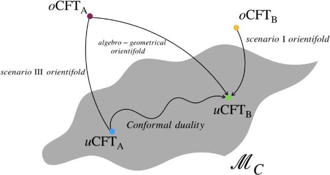
Here we present an algebraic-geometrical interpretation of orientifold, motivated by Greene's flop transition and the search for a quantum geometry [20-23], as morphisms between algebraic varieties. Orientifolds are thought of as maps that act both on the states of the theory and on the CY cones geometry. The net effect is an RG flow towards the IR regime, from the original oriented model to an unoriented one (see figure 9 to have a schematic picture in mind).
In section 2.1, we review toric varieties and toric CY discussing the construction of manifolds as an algebraic subvariety of the complex space, while in section 2.2 we review orientifold projection and its possible scenarios. In sections 3 and 4 we discuss the algebro-geometrical interpretation of the orientifold and the possible way RG flows triggered by the orientifold itself can be holographically interpreted.
2. Background material: toric geometry and orientifold
2.1. Toric varieties and toric Calabi-Yau
Toric geometry is a branch of algebraic geometry and a toric variety is, by definition, an algebraic variety containing an algebraic torus as an open dense subset, such that the action of the torus on itself extends to the whole variety. To be more specific, an n-dimensional toric variety ${ \mathcal M }$ has an algebraic torus action in the sense that the algebraic torus ${{\mathbb{T}}}^{n}={\left({{\mathbb{C}}}^{* }\right)}^{n}$ is a dense open subset and there is an action ${{\mathbb{T}}}^{n}\times { \mathcal M }\to { \mathcal M }$. The greatest point in favor of toric geometry is that the geometry of a toric variety is fully determined by combinatorics.
In the case of a toric CY variety, the information about the geometry is summarized in the so-called toric diagram which is a polytope embedded in a ${{\mathbb{Z}}}^{n-1}$-lattice. Moreover, when we consider a toric CY threefold cone the action of the algebraic torus enlarges the isometry group of the variety from U(1), the action induced by the Reeb vector field, to $U{\left(1\right)}^{3}$. Let us briefly review some possible constructions of toric varieties [2-4].
2.1.1. Homogeneous coordinates approach to toric varieties
The simplest way we can image toric variety is as a generalization of weighed projective space [24]. Let us recall first the definition of the (m − 1)-dimensional weighed projective space
where the quotient by ${{\mathbb{C}}}^{* }$ is taken into account by the identification $({z}_{1},\ldots ,{z}_{m})\sim ({\lambda }^{{i}_{1}}{z}_{1},\ldots ,{\lambda }^{{i}_{m}}{z}_{m})$ where $\lambda \in {{\mathbb{C}}}^{* }$ and (i1,…,im) are the so-called coordinates weights. An n-dimensional toric variety ${ \mathcal M }$ is the generalization where we quotient by more than one ${{\mathbb{C}}}^{* }$ action and the set that we subtract is a subset UΣ which contains not only the origin
$\begin{eqnarray}{ \mathcal M }=\displaystyle \frac{{{\mathbb{C}}}^{m}\setminus \{{U}_{{\rm{\Sigma }}}\}}{{\left({{\mathbb{C}}}^{* }\right)}^{m-n}\times {\rm{\Gamma }}},\end{eqnarray}$
where Γ is an abelian group. This variety has an algebraic torus action given by ${\left({{\mathbb{C}}}^{* }\right)}^{m-m+n}={\left({{\mathbb{C}}}^{* }\right)}^{n}$. Definition (2) emerges in the context of cones and fans that we are going to discuss.
Let M and N be dual n-dimensional lattices isomorphic to ${{\mathbb{Z}}}^{n}$ and consider the vector spaces ${M}_{{\mathbb{R}}}$ and ${N}_{{\mathbb{R}}}$ to be the subspace of ${{\mathbb{R}}}^{n}$ spanned, respectively, by vectors in M and N. We define the Strongly Convex Rational Polyhedral Cone (SCRPC) $\sigma \in {N}_{{\mathbb{R}}}\subset {{\mathbb{R}}}^{n}$ as the set
for a finite number of vectors vi and satisfying the condition (σ) ∩ ( − σ) = {0}. Let us analyze this definition: we consider an n-dimensional lattice $N\simeq {{\mathbb{Z}}}^{n}$, a SCRPC is an n or lower dimensional cone in ${N}_{{\mathbb{R}}}$ with the origin of the lattice as its apex, bounded by hyperplanes (polyhedral) with its edges spanned by lattice vectors (rational) and such that it does not contain complete lines (strongly convex). The dimension of a SCRPC σ is the dimension of the smallest subspace of ${{\mathbb{R}}}^{n}$ containing σ. Two important concepts are useful in SCRPC theory:
•
edges: these are the one-dimensional faces of σ, the vectors $\vec{g}$ associated with the edges are the generators of σ;
•
facets: these are the codimension one faces.
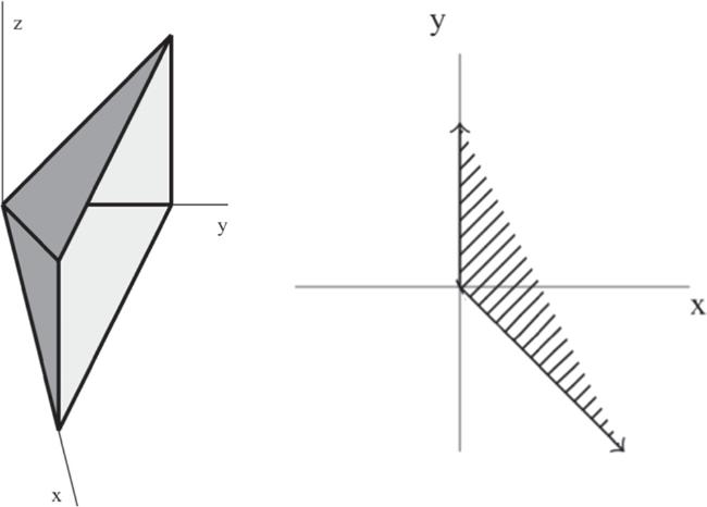
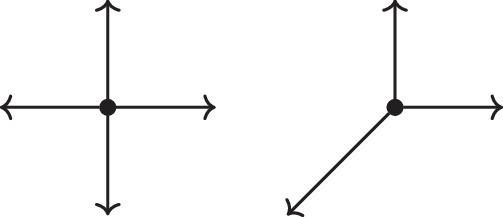
A collection Σ of SCRPCs in ${N}_{{\mathbb{R}}}$ is called a fan if each face of the SCRPC in Σ is also an SCRPC in Σ and the intersection of two SCRPCs in Σ is a face of each. Examples of SCRPCs and fans are reported in figures 1 and 2.
Figure 1. Examples of SCRPCs. Left: SCRPC in ${{\mathbb{R}}}^{3}$, its one dimensional faces are identified by the vectors ${\vec{g}}_{1}=(1,0,0),{\vec{g}}_{2}=(0,1,0),{\vec{g}}_{3}=(0,1,1),{\vec{g}}_{4}=(1,0,1)$ in ${{\mathbb{Z}}}^{3}$. Right: SCRPC in ${{\mathbb{R}}}^{2}$, its one-dimensional faces are identified by the vectors ${\vec{g}}_{1}=(0,1),{\vec{g}}_{2}=(1,-1)$ in ${{\mathbb{Z}}}^{2}$.
Figure 2. Examples of fans. Left: fan of ${{\mathbb{CP}}}^{1}\times {{\mathbb{CP}}}^{1}$, we have four one-dimensional SCRPCs (the vectors) and four two-dimensional SCRPCs (the quadrants). Right: fan of ${{\mathbb{CP}}}^{2}$, we have three one-dimensional SCRPCs (the vectors) and three two-dimensional ones (the trians).
Let us consider a fan Σ and we call Σ1d the set of one-dimensional SCRPCs; let ${\vec{v}}_{i}$ with i = 1,…,m be the whole set of vectors generating the one-dimensional SCRPCs in Σ1d.1(1 Note that obviously, m is equal to the number of one-dimensional cones and so to the number of elements in Σ1d.) To each vector ${\vec{v}}_{i}$ we associate a homogeneous coordinate ${z}_{i}\in {\mathbb{C}}$ and we define the set
where the union is taken over all the sets having I ⫅ {1,…,m} for which zi with i ∈ I does not belong to an SCRPC in Σ.
At this point, we need to discuss how the ${\left({{\mathbb{C}}}^{* }\right)}^{m-n}\times {\rm{\Gamma }}$ acts on ${{\mathbb{C}}}^{m}$. First of all, let us clarify the nature of the abelian group Γ: this is given by
where $\tilde{N}\subseteq N$ is the sublattice generated over ${{\mathbb{Z}}}^{n}$ by the vectors ${\vec{v}}_{i}$. In other words, vectors ${\vec{v}}_{i}$ not necessarily generate all N, in general they generate only $\tilde{N};$ on the one hand, if $\tilde{N}=N$ then Γ is trivial and does not play any role. On the other hand, if Γ is not trivial our variety develops orbifold singularity.
Let us now discuss the algebraic torus ${\left({{\mathbb{C}}}^{* }\right)}^{m-n}$ action. Consider the n × m matrix build-up considering the m vectors ${\vec{v}}_{i}$ with n components
Thanks to the rank-nullity theorem2(2Given T a linear map between two finite dimensional vector spaces A and B we have that ${\dim }({Im}(T))+{\dim }({Ker}(T))={Rank}(V)+{Null}(V)={\dim }(A)$. In our case we know that ${\vec{v}}_{i}$ with i=1,…,m are m linearly independent vectors so ${Rank}(V)={\dim }({Im}(T))=m$.) the dimension of the Kernel of map (7) must be m − n; we can identify it with ${\left({{\mathbb{C}}}^{* }\right)}^{m-n}$. It is now simple to see how ${\left({{\mathbb{C}}}^{* }\right)}^{m-n}$ acts on ${{\mathbb{C}}}^{m}$: each ${{\mathbb{C}}}^{* }$ action is taken into account by
with $\lambda \in {{\mathbb{C}}}^{* }$. We have m − n actions like (8), where for each a = 1,…,m − n the charge vectors ${Q}^{a}=({Q}_{1}^{a},\ldots ,{Q}_{m}^{a})$ belong to the Kernel of the map φ and therefore must satisfy m − n relations
$\begin{eqnarray}{ \mathcal M }=\displaystyle \frac{{{\mathbb{C}}}^{m}\setminus \{{U}_{{\rm{\Sigma }}}\}}{{\left({{\mathbb{C}}}^{* }\right)}^{m-n}\times {\rm{\Gamma }}};\end{eqnarray}$
this is an n-dimensional variety, with a residual ${\left({{\mathbb{C}}}^{* }\right)}^{n}\simeq U{\left(1\right)}^{n}$ action and the ${\left({{\mathbb{C}}}^{* }\right)}^{m-n}$ action is quotient out by m − n relations (10) with weights that satisfy relations (9). Let us give an example.
2.1.2. Example: ${{\mathbb{CP}}}^{2}$
Let us consider the right fan in figure 2: this is a ${{\mathbb{Z}}}^{2}$ lattice; we have the three vectors ${\vec{v}}_{1}=(0,1),{\vec{v}}_{2}=(1,0),{\vec{v}}_{3}=(-1,-1)$ that generate one-dimensional cones. We have three homogeneous coordinates $({z}_{1},{z}_{2},{z}_{3})\in {{\mathbb{C}}}^{3}$ and the set UΣ is given by the origin. Since m = 3 and n = 2 we must have one ${{\mathbb{C}}}^{* }$ action and we can find the weights using (9):
${{\mathbb{C}}}^{* }$ action is taken into account by the equivalence relation (z1, z2, z3) ∼ λ(z1, z2, z3). Finally, we note that the vectors ${\vec{v}}_{1}$ and ${\vec{v}}_{2}$ generate the whole lattice ${{\mathbb{Z}}}^{2}$ and so Γ is trivial. The toric variety corresponds to
$\begin{eqnarray}{ \mathcal M }=\displaystyle \frac{{{\mathbb{C}}}^{3}\setminus \{0\}}{{{\mathbb{C}}}^{* }}\equiv {{\mathbb{CP}}}^{2},\end{eqnarray}$
as we expected.
We now give some interesting properties about toric varieties and their fans:
•
a fan Σ is smooth if every SCRPC in Σ is smooth, an SCRPC is smooth if is generated by a subset of a basis of $N\simeq {{\mathbb{Z}}}^{n};$
•
a fan Σ is simplicial if every SCRPC in Σ is simplicial, an SCRPC is simplicial if it is generated by a subset of a basis of ${{\mathbb{R}}}^{n};$
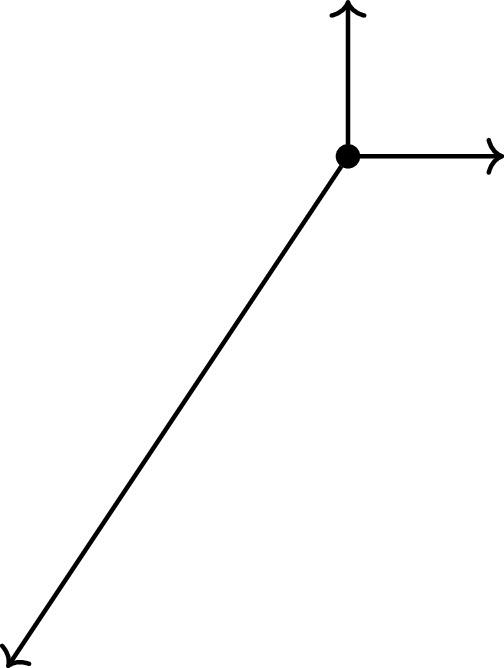
These conditions are important since if a fan is smooth the corresponding toric variety also is smooth and if a fan is simplicial then the corresponding toric variety can have at most orbifold singularities. We see immediately that the two spaces described by the fans in figure 2 are smooth since every SCRPC is generated by a subset of a ${{\mathbb{Z}}}^{2}$ basis. An example of toric variety with orbifold singularities is the weighted projective space ${{\mathbb{CP}}}_{\mathrm{2,3,1}};$ its fan is given in figure 3 below. Orbifold singularities can be removed by the so-called blow up procedure: roughly speaking, for an n-dimensional toric variety we replace the singular locus with ${{\mathbb{CP}}}^{n-1}$.
Figure 3. Fan of ${{\mathbb{CP}}}_{\mathrm{2,3,1}}$, we have ${\vec{v}}_{1}=(1,0),{\vec{v}}_{2}=(0,1),{\vec{v}}_{3}\,=(-2,-3)$. It is not smooth but it is simplicial: ${{\mathbb{CP}}}_{\mathrm{2,3,1}}$ has orbifold singularities.
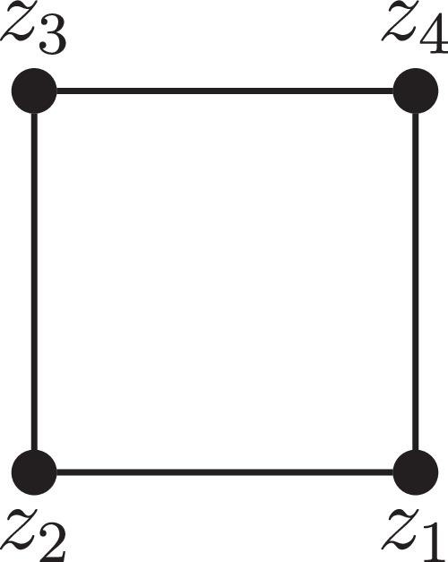
Figure 5. Toric diagram of $\tfrac{{{\mathbb{C}}}^{2}}{{{\mathbb{Z}}}_{2}}\times {\mathbb{C}}$.
Let us now specialize to the case of our interest: CY threefolds. First of all, we have an $U{\left(1\right)}^{3}\simeq {\left({{\mathbb{C}}}^{* }\right)}^{3}$ action but there is more: the condition of trivial canonical bundle implies that all the vectors of the fan belong to the same hyperplane, so we can project on this hyperplane obtaining a two-dimensional object whose convex hull takes the name of toric diagram. The CY condition implies
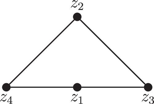
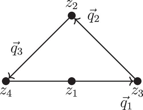
Consider the three-dimensional fan given by the four vectors ${\vec{v}}_{1}=(0,0,1),{\vec{v}}_{2}=(1,0,1),{\vec{v}}_{3}=(0,1,1),{\vec{v}}_{4}=(1,1,1)$. We note that these vectors belong to the same hyperplane, so we can project out the third component: we obtain ${\vec{w}}_{1}=(0,0),{\vec{w}}_{2}=(1,0),{\vec{w}}_{3}=(0,1),{\vec{w}}_{4}=(1,1)$. Hence the conifold is a CY variety and its toric diagram is given in figure 4.
We have m − n = 4 − 3 = 1 charge vector given by relation (9):
and a possible solution is Q = ( − 1, 1, 1, − 1). As one can note the CY condition is automatically implemented by the fact that the vectors are coplanar. The action of the algebraic torus ${{\mathbb{C}}}^{* }$ is quotient out by the equivalence relation
are invariant and this is the minimal basis with which to write all the ${{\mathbb{C}}}^{* }$-invariant polynomials. However, note that these polynomials are not independent but they must satisfy the relation
Consider the fan generated by the vectors ${\vec{v}}_{1}=(0,0,1),{\vec{v}}_{2}=(0,1,1),{\vec{v}}_{3}=(1,0,1),{\vec{v}}_{4}\,=(-1,0,1);$ projecting out the third component we get ${\vec{w}}_{1}=(0,0)$, ${\vec{w}}_{2}=(0,1)$, ${\vec{w}}_{3}=(1,0)$, ${\vec{w}}_{4}=(-1,0)$ and the toric diagram is given in figure 5.
and so Q = ( − 2, 0, 1, 1). Since we have one vanishing component, Q2 = 0, the coordinate z2 has no role and so we will expect a CY toric manifold of the form $X\times {\mathbb{C}}$, where X is unknown for the moment and ${\mathbb{C}}$ is the space associated to z2. We have the equivalence relation
since on z2 the algebraic torus action is trivial we do not consider it and so we must find m − 1 = 4 − 1 = 3 ${{\mathbb{C}}}^{* }$-invariant polynomials, for example
Relation (22) is the realization of $\tfrac{{{\mathbb{C}}}^{2}}{{{\mathbb{Z}}}_{2}}$ as subvariety of ${{\mathbb{C}}}^{3}$. In the end, the toric CY variety is $\tfrac{{{\mathbb{C}}}^{2}}{{{\mathbb{Z}}}_{2}}\times {\mathbb{C}}$.
The general algorithm to identify to which variety a toric diagram belongs is the following: given the toric diagram we look at the equivalent relations that quotient out the algebraic torus action ${\left({{\mathbb{C}}}^{* }\right)}^{m-n}$ and we construct a minimal basis of m${\left({{\mathbb{C}}}^{* }\right)}^{m-n}$-invariant polynomials; the m − n relations that these polynomials must satisfy identify the toric variety as subvariety of ${{\mathbb{C}}}^{m}$.
2.1.5. Moment maps approach and Delzant-like construction
Let us take a step back and consider a different way to define toric varieties. Let ${ \mathcal M }$ be a symplectic manifold of real dimension 2n with symplectic form ω. Given the action $U{\left(1\right)}^{n}\times { \mathcal M }\to { \mathcal M }$ this is said to be Hamiltonian if its restriction to any $U(1)\subset U{\left(1\right)}^{n}$ is Hamiltonian and any two of them commute. In this context the so-called moment map $\mu :{ \mathcal M }\to {{\mathbb{R}}}^{n}$ emerges, whose components are the Hamiltonians of each U(1) action. Since all the U(1) commute, for any $\vec{r}\in {{\mathbb{R}}}^{n}$, its preimage ${\mu }^{-1}(\vec{r})$ is invariant under the action of the full $U{\left(1\right)}^{n}$. Moreover, if ${ \mathcal M }$ has a Kähler structure, the existence of the Hamiltonian action implies that the isometry group contains the algebraic torus $U{\left(1\right)}^{n}\simeq {\left({{\mathbb{C}}}^{* }\right)}^{n}$. So a toric variety emerges in a simple way as a real 2n dimensional symplectic manifold ${ \mathcal M }$ that has a Hamiltonian action of the algebraic torus on it.3(3There is a little caveat: if ${ \mathcal M }$ is a cone the algebraic torus action must commute with the homothetic action induced by the Euler vector field.)
We are interested in non-compact toric varieties but let us talk a little about compact ones. If ${ \mathcal M }$ is compact, Delzant [25] showed that the image through the moment map of the variety, $\mu ({ \mathcal M })$, is a convex polytope Δ called Delzant polytope; however, we are interested in CY cones, i.e. non-compact toric varieties. The generalization to a Deltzan-like construction is possible [26] but the image under the moment map is no longer a polytope but a cone:
and its dual graph is still a fan generated by the normal vectors ${\vec{v}}_{i}$. CY condition imposes that ${\vec{v}}_{i}$ are coplanar so we can project out the common component and get an (n − 1)-dimensional object that encodes the geometry: the toric diagram. Since the components of the vectors ${\vec{v}}_{i}$ are integers, the toric diagram is the convex hull of a set of points in a ${{\mathbb{Z}}}^{n-1}$-lattice. In the Deltzan-like approach, the toric variety is built up using the Kähler quotient and the toric variety is a $U{\left(1\right)}^{n}$ fibration over Θ: one $U(1)\subset U{\left(1\right)}^{n}$ shrinks on the edges and so acts trivially, moreover, since in a vertex n edges meet each other, the full $U{\left(1\right)}^{n}$ fiber shrinks. Hence the vertexes are the fixed loci of the full algebraic torus action. It is interesting to note that this construction is well known by physicists: this is the moduli space of the Gauged Linear Sigma Model (GLSM), it is a SUSY gauge theory with abelian gauge group $U{\left(1\right)}^{m-n}$ and m chiral superfields Z1,…,Zm with charges Q1,…,Qm−n under the m − n U(1).
In the case of our interest, namely CY threefold, the toric diagram is a two-dimensional object and the CY cone threefold exhibits a three-dimensional algebraic torus action. From the toric diagram, we can get information on the dual QFT using the five brane system and brane tiling constructions; moreover, we can calculate some useful quantities of the dual field theory directly from the toric diagram, such as the central charge, using the Butti and Zaffaroni procedure [27] or the symplectic decomposition procedure [28].
2.2. Orientifold projections
Denoting by 0 ≤ σ ≤ π the coordinate describing the open string at a given time, the two ends σ = 0, π contain, thanks to Chan-Paton indexes, the gauge group degrees of freedom and the corresponding charged matter fields. At the endpoints, we can apply Dirichlet or Neumann boundary conditions and we know that under T-duality these are interchanged. Orientifold projections of Type IIB theory are obtained by projecting the Type IIB spectrum by the involution Ω (Ω2 = 1), exchanging the left and right closed oscillators ${\hat{\alpha }}_{m}^{\mu }$, ${\hat{\beta }}_{m}^{\mu }$ and acting on the open strings as phases:
The overall effect is that orientifold projections map oriented strings to unoriented ones and type I superstring theory is nothing but an orientifold projection of type IIB superstring theory [29]: $\mathrm{type}\ \ \ {\rm{I}}=\tfrac{\mathrm{type}\ \ \ \mathrm{IIB}}{{\rm{\Omega }}}$.
Orientifold introduces, from the worldsheet point of view, new surfaces in the Polyakov topological expansion. Indeed, due to the presence of unoriented strings, non-orientable surfaces such as Klein bottles or Möbius strips are allowed. From the space-time viewpoint, these correspond to not dynamical objects, called O-planes, defined by T-duality as fixed points of the orientifold projection [30].
However this picture is not the complete one since, nowadays, there are no results in actual string theory for what one might expect to be the curved back-reacted geometry of orientifold. Indeed as reported in [31], for any solution with O-planes, the presence of such a plane is inferred by comparison with their flat-space behavior. However, since the orientifolded space times have strong curvature and coupling, stringy corrections come into play, and it is impossible to decide with supergravity alone whether the solutions are valid. Therefore, it is natural to think of more general behaviors in which geometric phase transitions due to the presence of an orientifold can play a crucial role. Since this kind of behavior is highly non-perturbative we expect something to happen in the field theory that goes beyond the large N limit.
This orientifold construction has important consequences on the emergent field theory build up with the AdS/CFT and toric CY machinery: some degrees of freedom are projected out and orthogonal and symplectic groups are now allowed together with symmetric and antisymmetric representations of unitary groups. The rules for the construction of these kinds of theories are studied for example in [17, 32-34]. The crucial point here is that orientifold can give rise to different scenarios:
•
in scenario I there is a new superconformal fixed point and the R-charges of the operators that are not projected out by Ω are the same as the charges of the corresponding one in the oriented theory and in the large N limit. In the end, the post-orientifold central charge aΩ turns out to be half of the pre-orientifold central charge a;
•
scenario II does not admit a new superconformal RG fixed point;
•
in scenario III there is a new superconformal fixed point but the R-charges of the operators that are not projected out by Ω are different from the charges of the corresponding one in the oriented theory and not only at large N. In the end, the post-orientifold central charge aΩ turns out to be less than half of the pre-orientifold central charge a. However, something very interesting happens here: this could be (one of) the right field theory dual to the non-perturbative action of orientifold in the string theory side.
2.2.1. The scenario I orientifold
The scenario I orientifold occurs when the pre and post-orientifold R-charges of the theories are the same and the central charge post-orientifold is half of that pre-orientifold:
The CY cone describing the theory before and after the orientifold is then the same but with different volume due to the orientifold action. Moreover, due to the c-theorem in 4D, according to which aIR < aUV, the scenario I orientifolds lead to the IR regimes of the theory.
2.2.2. The scenario II orientifold
Scenario II seems to be quite trivial: there is no new superconformal point and the orientifold breaks conformal symmetry. However, as known in the literature, these situations can give rise to a duality cascade or conformal symmetry can be restored with flavor branes [35].
2.2.3. The scenario III orientifold and the IR duality
In the scenario III orientifold, the pre and post-orientifold R-charges of the theory are not the same and the post-orientifold central charge is less than half of that pre-orientifold [18, 19]:
In this case the CY cones describing the theory before and after the orientifold are not the same. Scenario III orientifold seems to be part of a bigger picture where geometry/topology transitions play a crucial role. Note that, since the c-theorem in 4D tells us that aIR < aUV, also scenario III orientifolds lead to the IR regimes of the theory.
3. Algebro-geometrical orientifold and IR dualities
The IR duality we are talking about was recently proposed in [18] studying the orientifold projections of Pseudo del Pezzo models (PdP) and subsequently extended to an infinite class of models in [19]. Given two different oriented models oCFTA and oCFTB, which have nothing to do with one another, it turns out that the existing orientifold projections are such that the R-charges, central charges and superconformal indexes of the two unoriented uCFTA and uCFTB models are the same [18, 19]
$\begin{eqnarray}{a}_{i}^{{\rm{\Omega }}}={b}_{i}^{{\rm{\Omega }}}={b}_{i},\ {a}_{A}^{{\rm{\Omega }}}={a}_{B}^{{\rm{\Omega }}}=\displaystyle \frac{{a}_{B}}{2},{{ \mathcal I }}_{A}^{{\rm{\Omega }}}={{ \mathcal I }}_{B}^{{\rm{\Omega }}}.\end{eqnarray}$
This suggests the proposed duality and since orientifold leads to the IR regime, this is an IR duality. More specifically the oCFTA has a scenario I orientifold while the oCFTB has a scenario III orientifold and the set of R-charges, central charges and superconformal indexes of the two unoriented models are the same for any finite value of N. What we have said in words is summarized in the following scheme.
Some examples of the IR duality due to orientifold in scenario III seems to be explained and interpreted, from the field theory point of view, in terms of inherited S-duality from the ${ \mathcal N }=2$ case. The authors observe that the duality for the ${ \mathcal N }=1$ models discussed in [19] corresponds to S-duality at different points of the conformal manifold [36-38]. Therefore the duality between the two unoriented models can be thought of as a conformal duality. The crucial property behind this result is the presence in the spectrum of two-index tensor fields with R-charge equal to one, uncharged with respect to the other global symmetries.
Our main goal is to better understand the link between orientifolds and the IR duality from the point of view of the geometry. The guiding ideas are the flop transition and the other geometry/topology changes in string theory compactifications, where the geometry/topology of the CY manifold are modified due to a quantum behavior of the geometry itself [20-23]. Heuristically, one suspects that geometry/topology might be able to change by means of violent curvature fluctuations, such as induced by an orientifold, which would be expected in any quantum theory of gravity. Therefore, the basic idea is that orientifold projections map the algebraic equations describing the geometry of the CYA into those that describe the geometry of the CYB. This orientifold modifies the geometry of the CYA cone due to its intrinsic non-perturbative nature and this geometrical change induces k new degrees of freedom with R-charges ${\tilde{a}}_{i}$ to emerge (we will call them orientifold-mapping operators or oμ-operators). They make the original field theory no longer fulfilling the condition ${\sum }_{1}^{d}{a}_{i}+{\sum }_{1}^{k}{\tilde{a}}_{i}=2;$ hence old R-charges ai and oμ-operators R-charges ${\tilde{a}}_{i}$ must mix together to return a set of new R-charges ${a}_{i}^{{\rm{\Omega }}}={b}_{i}$ consistent with the modified CY${}_{{\rm{A}}}^{{\rm{\Omega }}}$ cone geometry, that is now CYB cone, and satisfying the condition ${\sum }_{1}^{d}{b}_{i}=2$. The steps are summarized in the following scheme.
The procedure is as follows: from toric diagrams of theories A and B we determine the sets of algebraic equations using toric geometry tools exposed in section 2.1; then we map these two sets into each other and, finally, we associate at every homogeneous coordinate zi a trial R-charge, adding the minimal number of new degrees of freedom. The analysis must consider two different cases:
${P}_{e}^{(\bullet )}$ is the number of extremal points of the toric diagram of the theory •. Since in the oriented theory, only the trial R-chagres associated with extremal points matter, in the first case the two oriented theories have the same number of R-charges while in the second case the number of R-charges of the oriented theories are not equal and we expect that some not extremal points of the toric diagram of theory A became extremal points after the orientifold action. Cases with ΔPe > 1 are not discussed in this work since no examples have been found; they may be studied in future works to better understand the link between geometry, orientifold and the IR duality.
The interpretation of an orientifold in this way will be called an algebro-geometrical orientifold. This orientifold is different from scenario I and III orientifolds because, referring to scheme (29), the latter acts horizontally while the former acts crosswise from the oriented model A to the unoriented model B. This kind of orientifold implements the IR duality from the geometric point of view as morphism between CY algebraic varieties.
In the following subsection, we study these two cases with specific examples but this construction can be repeated for many other pairs and the result is that it is always possible to construct relevant operators with the new degrees of freedom inserted by matching the systems containing the polynomial equations that define the geometries of the pair.
3.1. Different number of external points: ΔPe = 1
Let us consider the conifold ${ \mathcal C }$ and $\tfrac{{{\mathbb{C}}}^{2}}{{{\mathbb{Z}}}_{2}}\times {\mathbb{C}};$ for toric diagrams and toric data. We refer to examples in subsection 2.1.4. Moreover, in those examples determination of the equations that describe the CY cones has already been done. The conifold has scenario I orientifold while $\tfrac{{{\mathbb{C}}}^{3}}{{{\mathbb{Z}}}_{2}}$ has scenario III orientifold and the two theories are IR duals. The set of equations for the two theories are
Now we have to map the two equations in all possible ways remembering that after the orientifold action the toric diagrams are mapped into each other and so the coordinates zi are effectively the same. However, if we want to keep track of the different R-charges associated to the homogeneous coordinate zi of the two different toric diagrams so the R-charges ${b}_{i}={b}_{i}^{{\rm{\Omega }}}$ and ai, we must remember that we have to associate a different set of R-charges at those zi belonging to different equations and so different theories. We have to consider the following mappings:
By associating the set of oriented R-charges {z1, z2, z3, z4} → {0, a2, a3, a4} to the zi coordinates of Yi polynomials and the set of oriented R-charges {z1, z2, z3, z4} → {b1, b2, b3, b4} to the zi coordinates of Xi polynomials, we get the following relations:
and we have also the relation ${\sum }_{i=1}^{4}{b}_{i}=2$. These conditions are not sufficient to fix unequivocally the values of the R-charges to those of the conifold. However this is right, indeed using the fact we know the values at the superconformal fixed point of the two sets of R-charges, namely {a1, a2, a3, a4} = {0, 2/3, 2/3, 2/3} and {b1, b2, b3, b4} = {1/2, 1/2, 1/2, 1/2}, we may note that the equations (32) do not do the right job. Nevertheless, if we admit the existence of a new operator (an orientifold-mapping operator) with R-charge $\tilde{a}=\tfrac{1}{3}$ we note that, for example,
Finally, let us now consider the fields associated to $\tfrac{{{\mathbb{C}}}^{2}}{{{\mathbb{Z}}}_{2}}\times {\mathbb{C}}$ and their R-charges [27, 28].
Hence we have 2 fields with R-charge a3, 2 fields with R-charge a2, 1 field with R-charge a4 and 1 field with R-charge a4 + a1. Despite in the oriented theory, charge a1 does not play any role, here, in the unoriented one, we can identify ${a}_{1}\equiv \tilde{a}$ and so there is a field with a new R-charge due to orientifold action; we call it Π.4(4 Its bosonic part will be dubbed puppon while its fermionic, one puchino. This field is the one associated, according to [27] or [28], to the R-charge given by the combination of the new charge entered in the game, $\tilde{a}$, and the other charges.)It is interesting to note that field Π associated with the R-charge ${a}_{4}+\tilde{a}$ has $R={a}_{4}+\tilde{a}=\tfrac{2}{3}+\tfrac{1}{3}=1$. We can build up a relevant deformation with Π, for example ${{ \mathcal O }}_{i}={{\rm{\Phi }}}_{i}{\rm{\Pi }}$ where Φi are the other chiral fields with R-charge $R[{{\rm{\Phi }}}_{i}]=\tfrac{2}{3}$. The scaling dimension of ${{ \mathcal O }}_{i}$ is given by ${{\rm{\Delta }}}_{{{ \mathcal O }}_{i}}=\tfrac{3}{2}R[{{ \mathcal O }}_{i}]=\tfrac{5}{2}\lt 3$. This makes sense given that orientifold has the effect of making the theory flow into the IR regime; so this operator turns on and the theory becomes IR dual to another theory that has the correct set of R-charges to match systems (32).
Figure 6. Toric diagram of $\tfrac{{{\mathbb{C}}}^{2}}{{{\mathbb{Z}}}_{2}}\times {\mathbb{C}}$ with the useful vectors to associate fields and R-charges.
Figure 7. Toric diagrams of $\tfrac{\mathrm{SPP}}{{{\mathbb{Z}}}_{2}}$ (right) and L(3,3,3) (left).
One may wonder since the mapping is not one-to-one; however this seems to be a peculiarity of very symmetric models described by highly symmetric toric diagrams with a small number of points. Indeed in the case of ${ \mathcal C }$ and $\tfrac{{{\mathbb{C}}}^{2}}{{{\mathbb{Z}}}_{2}}\times {\mathbb{C}}$ there are exactly four ways of superimposing the two toric diagrams so as to place the greatest number of points of the two diagrams in the same position. From the field theory point of view, this ambiguity is probably due to the flavour global symmetries of the models since in both the set of R-charges the R-charges themselves are identical.
3.2.Equal number of external points: ΔPe = 0
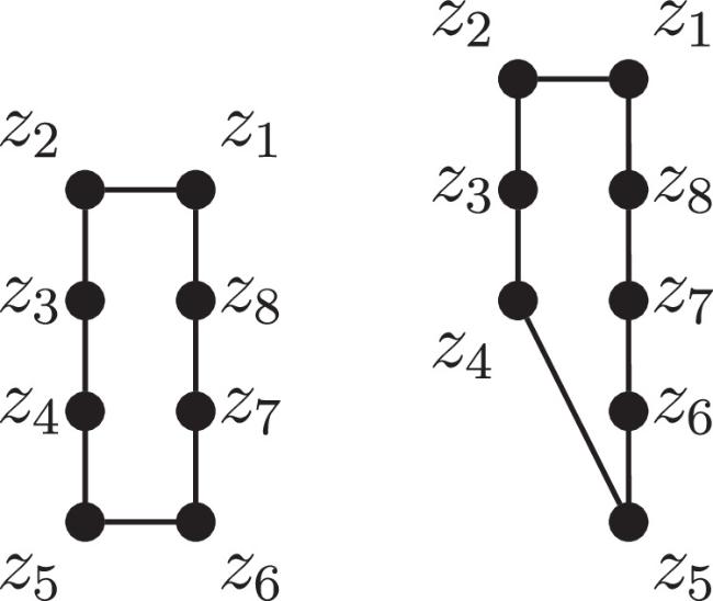
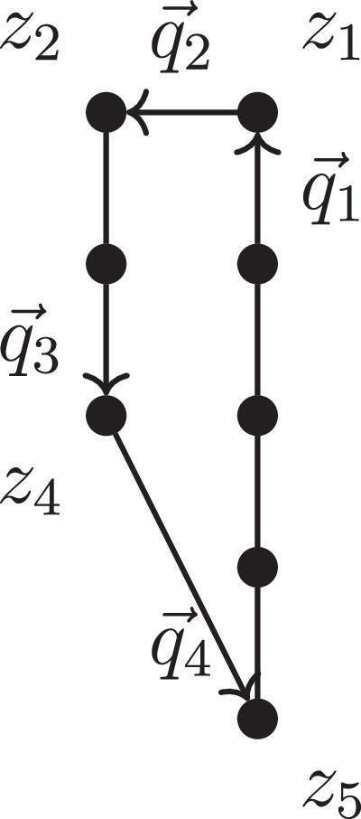
Consider the two theories $\tfrac{\mathrm{SPP}}{{{\mathbb{Z}}}_{2}}$ and L(3,3,3); their toric diagrams are drawn in figure 7.
To determine the set of equations describing the two varieties we follow the step highlighted in section 2.1.
Let us start with $\tfrac{\mathrm{SPP}}{{{\mathbb{Z}}}_{2}}$. We have m − n = 8 − 3 = 5 charge vectors solution of
where ${Q}_{1}^{a},{Q}_{2}^{a},{Q}_{3}^{a}$ satisfy (37). The 8 invariant polynomials can be constructed in a simple way: as the first step, we consider the homogeneous coordinates with not independent charges (in this case z1, z2, z3) and then we multiply them by the right combination of the other zi, in order to compensate the transformation under the equivalence relations; the second step is to build up the other polynomials taking product or quotient of polynomials constructed at the first step. This procedure not only gives us the invariant polynomials but also the relations between them. Invariant polynomials and relations are given by
Let us now proceed with the matching between sets (39) and (43). Since we have ΔPe = 0 we can not consider all the not extremal zi, indeed we expect that no new point enters the game. We note that if we match the first three polynomials of the two sets we get automatically that all other polynomials match, so
If we now consider the set of non-vanishing R-charges of $\tfrac{\mathrm{SPP}}{{{\mathbb{Z}}}_{2}}$ ($\{{a}_{1},{a}_{2},{a}_{3},{a}_{4}\}=\{1-\tfrac{1}{\sqrt{3}},1-\tfrac{1}{\sqrt{3}},\tfrac{1}{\sqrt{3}},\tfrac{1}{\sqrt{3}}\}$) and L(3,3,3) ($\{{b}_{1},{b}_{2},{b}_{3},{b}_{4}\}=\left\{\tfrac{1}{2},\tfrac{1}{2},\tfrac{1}{2},\tfrac{1}{2}\right\}$) we note that system (44) does not match unless we suppose the existence of a new operator (an orientifold-mapping operator) with R-charge $\tilde{a}=\tfrac{2-\sqrt{3}}{\sqrt{3}}$.
Following the same steps of the case ΔPe = 1 we can associate R-charges to the fields of theory $\tfrac{\mathrm{SPP}}{{{\mathbb{Z}}}_{2}}$.
In this case we do not have an obvious candidate to play the role of Π since no new extremal point enters in the game. Despite this, we can construct relevant operators that perturb the conformal theory and induce the RG flow to the dual theory in the IR. As in the ΔPe = 1 case, we add the new R-charge to the point that must be moved to transform the toric diagram of $\tfrac{\mathrm{SPP}}{{{\mathbb{Z}}}_{2}}$ into the toric diagram of L(3,3,3), namely z5. Therefore Π is a field with R-charge $R[{\rm{\Pi }}]={a}_{4}+\tilde{a}$ and a relevant operator can be constructed, for example, as ${{ \mathcal O }}_{i}={\rm{\Pi }}{\chi }_{i}$ where χi are the two fields with R-charge R[χi] = a1 + a2. The scaling dimension of ${{ \mathcal O }}_{i}$ is given by ${\rm{\Delta }}[{{ \mathcal O }}_{i}]=\tfrac{3}{2}R[{{ \mathcal O }}_{i}]=\tfrac{3}{2}\lt 3$.
Figure 9. Schematic picture of the RG flow triggered by the orientifold action. The little ‘o' stays for ‘oriented' while the little ‘u' stays for ‘unoriented'. The two unoriented models lie on the same conformal manifold while the two oriented models are not related in any way. The flow triggered by the algebro-geometrical orientifold action links the oriented model A to the unoriented model B.
In this case, we have only one matching which is suggested by the fact that we have only one way of superimposing the two toric diagrams so as to place the greatest number of points of the two diagrams in the same position. Indeed the toric diagrams are less symmetric with respect to the case of ${ \mathcal C }$ and $\tfrac{{{\mathbb{C}}}^{2}}{{{\mathbb{Z}}}_{2}}\times {\mathbb{C}}$ and the field theories have less flavour global symmetries.
4. Brief discussion on the holographic dual
In section 3 we have shown that, assuming the orientifold is able to change the geometry by transforming the CYA cone into the CYB cone we are forced to consider relevant operators which induce an RG flow that we know must end in a new superconformal fixed point. In holography, we are able to build up gravity solutions that are dual to RG flows [39].
4.1. The toy model for holographic duals of RG flows and beyond
Let us consider a set of scalar fields φa in an AdS5 background with coordinates (x0, x1, x2, x3, z)5(5We are going to use Greek indices for 4-dimensional quantities and capital Latin indices for 5-dimensional ones.) and action given by
We assume a 4D Poincaré invariant metric of the form ds = dz2 + e2Y(z)dxμdxμ, known as the domain wall ansatz, that we recognize as the Poincaré patch AdS with a radius R if the warp factor is a linear function $Y(z)=\tfrac{z}{R}$ and using the redefinition ${{\rm{e}}}^{\tfrac{z}{R}}=\tfrac{R}{z}$. Fields equations read
then the second equation is trivially satisfied while the first gives us ${\left({\partial }_{z}Y\right)}^{2}=-\tfrac{{V}_{\mathrm{crit}}}{3}$. Up to coordinates redefinition, we can then write as
This is nothing but AdS with its radius controlled by the critical point of the potential. Now we can expand the action around this solution and we can infer the conformal dimension of a CFT operator Oa from the masses of the quadratic fluctuations ma,
At this point we are looking for more generic solutions that are asymptotically AdS; we will consider solutions that have the linear warp factor $Y(z)=\tfrac{z}{R}$ and constant φa near the boundary at z → ∞ and in the deep interior for z → − ∞ . This is conjectured to be dual to an RG flow from a UV fixed point to an IR fixed point. It is natural to identify the radial coordinate z with the field theory RG scale via $\mu ={\mu }_{0}{{\rm{e}}}^{\tfrac{z}{R}}$, this choice guarantees that in the UV, at the AdS boundary, we have μ → ∞ for z → ∞ , while in the deep interior we have μ → 0 for z → − ∞ . As we know the exact identification of the RG scale is scheme dependent and a particular choice of coordinates on the supergravity side corresponds to a particular choice of renormalisation scheme on the field theory side. Said in another way, our goal is to find an interpolating flow solution of (46) which interpolates between two stationary points. In AdS/CFT language, this means that we are looking for a domain wall solution interpolating between an AdS space of radius RUV for z → ∞ and another AdS space of radius RIR for z → − ∞ . At the same time, the scalars φa are expected to flow from a constant ${\phi }_{{a}_{{UV}}}$ in the UV to a constant ${\phi }_{{a}_{{IR}}}$ in the IR. A domain wall solution of this type is expected to be dual to a field theory RG flow between two conformal theories.
Since for z → ± ∞ we have an AdS space-time we can use the holographic dictionary: on the boundary and in the deep interior region the scalars behave as
in which Aa is the source of Oa and Ba is its VEV. If Aa ≠ 0 the solution describes a deformation of the CFT by operator Oa while if Aa=0 and Ba ≠ 0 it describes a different vacuum of the CFT where the operator Oa develops a non-vanishing VEV. In both cases, conformal invariance is broken and an RG flow is triggered; the gravity solution is dual to this RG flow.
Particularly interesting is the case in which the Oa operator is relevant and the RG flow leads to a new fixed point and this is possible if and only if the potential V(φ) has more than one critical point (in such a way that another AdS solution with different radius is possible); the gravity solution is a kink interpolating between the two critical point AdS solutions. In order to have an RG flow that starts from a CFTUV we need a relevant operator (very similar to what happens in IR duality linked to the algebro-geometrical orientifold) and to hit a CFTIR we need the operator to become irrelevant there. Looking at the mass-dimension formula this means that in the relevant operator case, the squared mass of the scalar fluctuation must be negative (a maximum of the potential V(φ)) while in the irrelevant operator case, the squared mass must be positive (a minimum of the potential V(φ)).
The construction of holographic dual of RG flows could be applied to explain the IR duality arising from algebro-geometrical orientifold. We have seen how the duality requires the presence of relevant operators that deform the initial CFT associated with the CYA cone into the CFT associated with the CYB cone. In the spirit of the toy model presented above, this entire IR duality mechanism could be interpreted as the holographic dual of a suitable effective supergravity solution that has to interpolate between the supergravity solution of oriented model A and the supergravity solution of unoriented model B. Let us label the oriented models as oCFTA and oCFTB while the unoriented models as uCFTA and uCFTB. If we are able to perform the Kaluza-Klein (KK) reduction on the SE base manifolds ${X}_{{\rm{A}}}^{5}$ and ${X}_{{\rm{B}}}^{5}$ we get two gauged supergravity descriptions with two different potentials ${V}_{{X}_{{\rm{A}}}^{5}}$ and ${V}_{{X}_{{\rm{B}}}^{5}}$. We expect these two gauged supergravity theories are consistent truncations of type IIB superstring theory, respectively, on ${{AdS}}_{5}\times {X}_{{\rm{A}}}^{5}$ with gauge group ${G}_{{X}_{{\rm{A}}}^{5}}$ and on ${{AdS}}_{5}\times {X}_{{\rm{B}}}^{5}$ gauge group ${G}_{{X}_{{\rm{B}}}^{5}}$. This is in analogy with the FGPW flow [40], which is the holographic description of the Leigh-Strassler RG flow [41] of ${ \mathcal N }=4$ SYM theory. Moreover, as in the FGPW flow and according to AdS/CFT philosophy, we expect the gauge groups to be given by the isometry groups of the SE bases.
The flow would be holographically described if we are able to find a suitable supergravity description with a potential that has several critical points. The maximum of the potential has to preserve the original ${G}_{{X}_{{\rm{A}}}^{5}}$ symmetry while another critical point has to preserve the ${G}_{{X}_{{\rm{B}}}^{5}}$ symmetry. However, this kind of approach poses technical and conceptual challenges. First of all the KK reduction on the compact Sasaki-Einstein manifold X5 is far more difficult than for S5. Therefore, it is not easy at all to build up explicit potentials for these supergravity descriptions. Moreover, from the conceptual point of view, the supergravity description cannot be the full story since the orientifold is non-perturbative. The supergravity description has to be uplifted in a full string theory description which must match with the string theories associated with the two CFTs A and B. Anyway, it is not clear if such a suitable supergravity model exists but if so, we will have a holographic description of the flow induced by the algebro-geometrical orientifold itself and further investigation on this point will be part of future research works.
5. Conclusion
Orientifold projections give the opportunity of new possibilities for the creation of field theory models from a string background called unoriented models [13]. The appellation ‘unoriented' is mainly due to the action of the orientifold map on the string oscillators: the involution makes an oriented string an unoriented one and a Chan-Paton-like analysis suggests the possibility of a new gauge group like SO(N) and Sp(2N). However, orientifold behaviour is inferred by comparison with the flat-space behavior but, probably, orientifolds have an intrinsic non-perturbative nature [31]. This is also suggested by a recent interesting new feature proposed in [18] and expanded in [19]: the so-called scenario III. What happens is that a theory after a scenario III orientifold shares the same R-charges, central charge and superconformal index of another orientifolded theory coming from a scenario I orientifold. The crucial point is that these physical quantities are the same not only in the large N limit but for every N [18, 19]: this is a non-perturbative effect. Since the physical quantities are the same in the IR we refer to these theories as IR duals and, since in geometrical engineering, the field theory depends on the geometry of the CY cone, these two orientifolded theories can be considered to have the same CY cone geometry. This means that a change in the geometry of the cone has to happen due to the orientifold action. The change, due to the orientifold, can be traced back to the equations that describe the algebraic CY varieties and we require the matching between these sets of equations. In this sense, the orientifold has an algebro-geometrical interpretation as a morphism between algebraic varieties given locally by polynomials. This interpretation has as its guiding idea the flop transition and the other geometrical change in string theory compactifications [20-23]. The properties and a deeper understanding of this interpretation, such as the answers to the questions: ‘Are orientifold regular maps or rational maps? Are they biregular or birational?' could be fertile ground for future works. We stress that if orientifolds are such kinds of maps for the CY cones, they open the door to the use of the theory of category with orientifolds as morphisms and field theory as objects. Therefore, an orientifold acts both on string states and on the geometry of the space-time.
From the requirement of the matching between these sets of equations describing the CY cone of the two theories and using some tools of algebraic geometry and toric geometry, reported in 2.1, we infer the existence of relevant operators that deform the initial CFT triggering an RG flow towards the IR regime. A schematic picture of the flow is given in figure 9. The flow could be described using a holographic dual, whose toy model is presented in 4.1, but the prohibitive KK reduction on the base of a generic CY cone makes the explicit construction difficult. Moreover, due to the intrinsic non-perturbative nature of orientifold, this supergravity dual is expected to be only an effective description that must necessarily be uplifted in full string theory.
We thank first of all Prof. Fabio Riccioni for inspiring the present work and Prof. Massimo Bianchi and Salvo Mancani for interesting discussions. We also thank Davide Morgante for the discussions and comments and Matteo Romoli for their reading of the manuscript and comments. Special thanks to Maria Luisa Limongi who supported the work.
SagnottiA1987 Open strings and their symmetry groups NATO Advanced Summer Institute on Nonperturbative Quantum Field Theoryvol 9 Cargese Summer Institute
GreeneB R1996 String theory on Calabi-Yau manifolds Theoretical Advanced Study Institute in Elementary Particle Physics (TASI 96): Fields, Strings, and Duality 543 726
21
AspinwallP SGreeneB RMorrisonD R1994 Calabi-Yau moduli space, mirror manifolds and space-time topology change in string theory Nucl. Phys. B416 414
AmaritiABianchiMFazziMMancaniSRiccioniFRotaS2022${ \mathcal N }$=1 conformal dualities from unoriented chiral quivers J. High Energy Phys. JHEP09(2022)235
AmaritiABianchiMFazziMMancaniSRiccioniFRotaS2023 Multi-planarizable quivers, orientifolds, and conformal dualities J. High Energy Phys. JHEP09(2023)094


