


1. Introduction
Quantum droplets of atomic Bose gases have recently attracted great attention in the cold atom community [1-3]. For both dipolar [4-7] and binary condensates [8-13], it was found that a high density gas may stably exist even when the contact interactions was tuned to the regime where condensates become unstable. Since then, there have been tremendous experimental studies on the properties of the condensates in this regime [14-20]. On the theoretical side, a commonly used approach for studying quantum droplets is the extend Gross-Pitaevskii equation (EGPE) which perturbatively incorporates quantum fluctuation (i.e. Lee-Huang-Yang correction [21]) into the Gross-Pitaevskii equation [22-25]. However, to make work in the mean-field unstable regime, one has to ignore the imaginary part in the excitation spectrum. In addition, although EGPE has provided satisfactory explanations to experimental observations, there are still discrepancies with experimental measurements [3, 7, 8]. The properties of the quantum droplet were also studied with approaches beyond EGPE by taking into account the higher order corrections [26-30] or by employing the quantum Monte Carlo methods [31-35]. In any cases, as a perturbative treatment, the EGPE results should be checked with self-consistent calculations.
In a series of works [36-40], we studied the ground-state properties and the dynamics of the atomic condensates using the self-consistent Gaussian-state theory (GST) that takes account of the fluctuation at the Hartree-Fock-Bogoliubov level [41]. More importantly, GST gives rise to the gapless excitation spectrum of condensates [36, 42, 43], which remedies the flaw of the Hartree-Fock-Bogoliubov theory. As to the stabilization mechanism of the dipolar and binary droplets, our studies showed that they were stablized by the three-body repulsion, instead of the quantum fluctuation [37-39]. In particular, we found two new macroscopic squeezed states in droplets, i.e. the squeezed-vacuum state (SVS), squeezed-coherent state (SCS), other than the conventional coherent state (CS). Physically, these macroscopic squeezed states distinguish themselves from the CS state by having a large second-order correlation and an asymmetric atom-number distribution [36, 37], which allows the potential experimental detection of the new quantum phases. In addition, for quasi-two-dimensional (quasi-2D) droplets, we showed that the multiple quantum phases can be identified from the radial size versus atom number curve [38, 39]. As to the dynamics of the atomic condensates, we studied the collapse dynamics of a single-component condensate with attractive interaction [40]. It was shown that, starting from a coherent condensate, a small fraction of atoms can be transferred into the macroscopic squeezed state by tuning the contact interaction to sufficiently attractive [40].
By closely following the experimental configuration [9], we study, in this work, the ground-state properties and the dynamics of a quasi-one-dimensional (quasi-1D) binary Bose condensates using the Gaussian state theory. Compared to the quasi-2D counterpart, the quasi-1D system allows us to perform numerical simulations with high precision which is of particular importance for the dynamics. For the ground states of the condensates, we show that, in analog to the quasi-2D case, there exist three distinct phases, i.e. SVS, SCS, and CS. Particularly, we find that it is a crossover between the SCS and CS phases, in contrast to the first-order transition in quasi-2D systems. As to the dynamics, we show that, by tuning the reduced scattering length to a negative value, up to 60% of the total atoms can be transferred from a coherent state to a macroscopic squeezed state, which is in striking contrast to that found in single-component condensates.
The rest of this paper is organized as follows. In section 2 , we introduce our model and the GST for both imaginary- and real-time evolution. In section 3 , we present the results on the ground-state properties of a self-bound quasi-1D binary droplet, including the optimal number ratio, quantum phases, and axial width. In section 4 , we study the dynamics of a coherent condensate after the reduced interaction is tuned to attractive regime. In particular, we show that the macroscopic squeezing can be efficiently generated in this process. Finally, we conclude in section 5 .
2. Formulation
In this section, we first introduce our model for the quasi-1D droplet of Bose-Bose mixtures. Then we give a short review on GST. Particularly, we present the equations of motion for system in both imaginary and real times. We will also discuss the physical natures of the quantum states based on the Gaussian states.
2.1. Model
We consider a ultracold gas of N 39K atoms with N↑ atoms being in the hyperfine state $\left|\uparrow \right\rangle \equiv \left|F,{m}_{F}\right\rangle =\left|1,-1\right\rangle $ and N↓ in $\left|\downarrow \right\rangle \equiv \left|1,0\right\rangle $. The total Hamiltonian of the system
$\begin{eqnarray}H={H}_{0}+{H}_{2B}+{H}_{3B},\end{eqnarray}$
consists of the single-, two-, and three-particle terms In second-quantized form, the single-particle part reads $\begin{eqnarray}{H}_{0}=\displaystyle \sum _{\alpha }\int {\rm{d}}{\boldsymbol{r}}{\hat{\psi }}_{\alpha }^{\dagger }({\boldsymbol{r}})\left(-\frac{{\hslash }^{2}{{\rm{\nabla }}}^{2}}{2M}+{V}_{\mathrm{ext}}-{\mu }_{\alpha }\right){\hat{\psi }}_{\alpha }({\boldsymbol{r}}),\end{eqnarray}$
where ${\hat{\psi }}_{\alpha }\left({\boldsymbol{r}}\right)$ (α = ↑ , ↓ ) are the field operators, M is the mass of the atom $\begin{eqnarray}{V}_{\mathrm{ext}}(x,y)=\displaystyle \frac{1}{2}M{\omega }_{\perp }^{2}({x}^{2}+{y}^{2})\end{eqnarray}$
is the external trap on the transverse plane with ω⊥ being the radial trap frequency, and μα are the chemical potential introduced to fixed the mean atom numbers in both spin components. Moreover, the two-body (2B) interaction Hamiltonian takes the form $\begin{eqnarray}{H}_{2B}=\displaystyle \sum _{\alpha \beta }\frac{{g}_{\alpha \beta }}{2}\int {\rm{d}}{\boldsymbol{r}}{\hat{\psi }}_{\alpha }^{\dagger }({\boldsymbol{r}}){\hat{\psi }}_{\beta }^{\dagger }({\boldsymbol{r}}){\hat{\psi }}_{\beta }({\boldsymbol{r}}){\hat{\psi }}_{\alpha }({\boldsymbol{r}}),\end{eqnarray}$
where gαβ = 4πℏ2aαβ/M characterize the 2B interaction strengths with aαβ being scattering length between components α and β. The scattering lengths are tunable through Feshbach resonance and for scenario of interest to the binary droplets of 39K atom, the intra- and inter-species scattering lengths satisfy a↑↑, a↓↓ > 0 and a↑↓ < 0, respectively. The three-body (3B) interaction Hamiltonian can be expressed as $\begin{eqnarray}{H}_{3B}=\frac{{g}_{3}}{3!}\displaystyle \sum _{\alpha \beta \gamma }\int {\rm{d}}{\boldsymbol{r}}{\hat{\psi }}_{\alpha }^{\dagger }({\boldsymbol{r}}){\hat{\psi }}_{\beta }^{\dagger }({\boldsymbol{r}}){\hat{\psi }}_{\gamma }^{\dagger }({\boldsymbol{r}}){\hat{\psi }}_{\gamma }({\boldsymbol{r}}){\hat{\psi }}_{\beta }({\boldsymbol{r}}){\hat{\psi }}_{\alpha }({\boldsymbol{r}}),\end{eqnarray}$
where g3 is the 3B coupling constant which, for simplicity, is assumed to be spin independent. In order to stabilize the 2B attraction, we assume that g3 is positive.For the experimental configuration [9], the radial trap frequency is sufficiently large such that the motion of atoms on the transverse direction is frozen to the ground state of the transverse harmonic oscillator. As a result, we may factorize the field operators into1 ) reduces to a 1D form, i.e.
$\begin{eqnarray}{\hat{\psi }}_{\alpha }({\boldsymbol{r}})={\hat{\psi }}_{\alpha }(z)\frac{{{\rm{e}}}^{-({x}^{2}+{y}^{2})/(2{a}_{\perp }^{2})}}{{\left(\pi {a}_{\perp }^{2}\right)}^{1/2}},\end{eqnarray}$
where ${a}_{\perp }=\sqrt{{\hslash }/(M{\omega }_{\perp })}$ is the radial harmonic oscillator length. After integrating out the transverse motion, Hamiltonian ( $\begin{eqnarray}\begin{array}{rcl}\hat{H} & = & \displaystyle \sum _{\alpha }\int {\rm{d}}z{\hat{\psi }}_{\alpha }^{\dagger }(z){\hat{h}}_{\alpha }{\hat{\psi }}_{\alpha }(z)\\ & & +\,\displaystyle \sum _{\alpha \beta }\frac{{g}_{\alpha \beta }^{\prime} }{2}\int {\rm{d}}z{\hat{\psi }}_{\alpha }^{\dagger }(z){\hat{\psi }}_{\beta }^{\dagger }(z){\hat{\psi }}_{\beta }(z){\hat{\psi }}_{\alpha }(z)\\ & & +\frac{{g}_{3}^{\prime} }{3!}\displaystyle \sum _{\alpha \beta \gamma }\int {\rm{d}}z{\hat{\psi }}_{\alpha }^{\dagger }(z){\hat{\psi }}_{\beta }^{\dagger }(z){\hat{\psi }}_{\gamma }^{\dagger }(z){\hat{\psi }}_{\gamma }(z){\hat{\psi }}_{\beta }(z){\hat{\psi }}_{\alpha }(z),\end{array}\end{eqnarray}$
where ${\hat{h}}_{\alpha }=-{{\hslash }}^{2}{\partial }_{z}^{2}/(2M)-{\mu }_{\alpha }$ with an unimportant constant being absorbed into the chemical potential and ${g}_{\alpha \beta }^{\prime} ={g}_{\alpha \beta }/(2\pi {a}_{\perp }^{2})$ and ${g}_{3}^{\prime} ={g}_{3}/(3{\pi }^{2}{a}_{\perp }^{4})$ are, respectively, the reduced 2B and 3B interaction strengths in the quasi-1D geometry.2.2. GST for the ground states and dynamics of the condensates
For completeness, here we present a brief introduction to GST. A Gaussian-state wave function, ∣GS⟩, can be equivalently characterized using the coherent-state wave functions ${\phi }_{\alpha }^{(c)}(z)=\langle \mathrm{GS}| {\hat{\psi }}_{\alpha }(z)| \mathrm{GS}\rangle $, the normal correlation functions ${G}_{\alpha \beta }(z,z^{\prime} )=\langle \mathrm{GS}| \delta {\hat{\psi }}_{\beta }^{\dagger }(z^{\prime} )\delta {\hat{\psi }}_{\alpha }(z)| \mathrm{GS}\rangle $, and the anomalous correlation functions ${F}_{\alpha \beta }(z,z^{\prime} )=\langle \mathrm{GS}| \delta {\hat{\psi }}_{\beta }(z^{\prime} )\delta {\hat{\psi }}_{\alpha }(z)| \mathrm{GS}\rangle $, where $\delta {\hat{\psi }}_{\alpha }(z)={\hat{\psi }}_{\alpha }(z)-{\phi }_{\alpha }^{(c)}(z)$ is the fluctuation. To determine $\{{\phi }_{\alpha }^{(c)},{G}_{\alpha \beta },{F}_{\alpha \beta }\}$ for a ground state, we note that the total energy of the system can be expressed as
$\begin{eqnarray}E=\langle {{\rm{\Psi }}}_{\mathrm{GS}}| \hat{H}| {{\rm{\Psi }}}_{\mathrm{GS}}\rangle ={E}_{\mathrm{kin}}+{E}_{2B}+{E}_{3B},\end{eqnarray}$
where $\begin{eqnarray}\begin{array}{c}{E}_{\mathrm{kin}}=\displaystyle \sum _{\alpha }\int {\rm{d}}z\left[\Space{0ex}{1.27em}{0ex}{\phi }_{\alpha }^{(c)}{\left(z\right)}^{* }{\hat{h}}_{\alpha }(z){\phi }_{\alpha }^{(c)}(z)\right.\\ \,\left.+\mathop{\mathrm{lim}}\limits_{z^{\prime} \to z}{\hat{h}}_{\alpha }(z^{\prime} ){G}_{\alpha \alpha }(z^{\prime} ,z)\right]\end{array}\end{eqnarray}$
is the kinetic energy, $\begin{eqnarray}\begin{array}{rcl}{E}_{2B} & = & \displaystyle \sum _{\alpha \beta }\frac{{g}_{\alpha \beta }}{2}\int {\rm{d}}z\left\{\Space{0ex}{2.5ex}{0ex}{n}_{\alpha }(z){n}_{\beta }(z)\right.\\ & & +\,2\mathrm{Re}{\phi }_{\alpha }^{(c)}(z){\phi }_{\beta }^{(c)}(z){F}_{\alpha \beta }{\left(z,z\right)}^{* }+| {F}_{\alpha \beta }(z,z){| }^{2}\\ & & \left.+\,\left[2{\phi }_{\alpha }^{(c)}{\left(z\right)}^{* }{\phi }_{\beta }^{(c)}(z)+{G}_{\beta \alpha }(z,z)\right]{G}_{\alpha \beta }(z,z)\right\}\end{array}\end{eqnarray}$
is the two-body interaction energy, and $\begin{eqnarray}\begin{array}{r}{E}_{3B}=\frac{{g}_{3}}{3!}\displaystyle \sum _{\alpha \beta \gamma }\int {\rm{d}}z\left\{{n}_{\alpha }(z){n}_{\beta }(z){n}_{\gamma }(z)+6\mathrm{Re}{\phi }_{\alpha }^{(c)}(z){\phi }_{\beta }^{(c)}(z)\right.\\ \,\times \left[{n}_{\gamma }(z){F}_{\alpha \beta }{\left(z,z\right)}^{* }+2{F}_{\alpha \gamma }{\left(z,z\right)}^{* }{G}_{\gamma \beta }(z,z)\right]\\ \,+3\left[2{\phi }_{\alpha }^{(c)}{\left(z\right)}^{* }{\phi }_{\beta }^{(c)}(z){G}_{\alpha \beta }(z,z)+| {G}_{\alpha \beta }(z,z){| }^{2}\right]{n}_{\gamma }(z)\\ \,+2{G}_{\alpha \beta }(z,z){G}_{\beta \gamma }(z,z){G}_{\gamma \alpha }(z,z)\\ \,+6{\phi }_{\alpha }^{(c)}(z){\phi }_{\beta }^{(c)}{\left(z\right)}^{* }\left[{F}_{\alpha \gamma }^{* }(z,z){F}_{\beta \gamma }(z,z)\right.\\ \,\left.+{G}_{\beta \gamma }(z,z){G}_{\gamma \alpha }(z,z)\right]\\ \,\left.+3{F}_{\alpha \beta }(z,z)\left[{F}_{\alpha \beta }{\left(z,z\right)}^{* }{n}_{\gamma }(z)+2{F}_{\alpha \gamma }{\left(z,z\right)}^{* }{G}_{\gamma \beta }(z,z)\right]\Space{0ex}{2.2ex}{0ex}\right\}\end{array}\end{eqnarray}$
is the 3B interaction energy. Here ${n}_{\alpha }(z)=| {\phi }_{\alpha }^{(c)}(z){| }^{2}\,+{G}_{\alpha \alpha }(z,z)$ is the density of the αth spin component. Then, the ground-state wave function can be obtained by minimizing the total energy, which, in GST, is expressed as a set of evolution equations of $\{{\phi }_{\alpha }^{(c)},{G}_{\alpha \beta },{F}_{\alpha \beta }\}$ in imaginary time τ = it.To write out these equations in compact forms, we express $\{{\phi }_{\alpha }^{(c)},{G}_{\alpha \beta },{F}_{\alpha \beta }\}$ into a vector ${\phi }^{(c)}\equiv \left(\begin{array}{c}{\phi }_{\uparrow }^{(c)}\\ {\phi }_{\downarrow }^{(c)}\end{array}\right)$ and two matrices $G\equiv \left(\begin{array}{cc}{G}_{\uparrow \uparrow } & {G}_{\uparrow \downarrow }\\ {G}_{\downarrow \uparrow } & {G}_{\downarrow \downarrow }\end{array}\right)$ and $F\equiv \left(\begin{array}{cc}{F}_{\uparrow \uparrow } & {F}_{\uparrow \downarrow }\\ {F}_{\downarrow \uparrow } & {F}_{\downarrow \downarrow }\end{array}\right)$ in the spin space. Additionally, we introduce the vector $\eta \equiv \left(\begin{array}{c}{\eta }_{\uparrow }(z)\\ {\eta }_{\downarrow }(z)\\ \end{array}\right)$ with15 )-(17 ) should be summed over the repeated indices in the spin space and integrated over the repeated coordinates in the spatial space [39].
$\begin{eqnarray}\begin{array}{l}{\eta }_{\alpha }(z)={\hat{h}}_{\alpha }(z){\phi }_{\alpha }^{(c)}(z)+\displaystyle \sum _{\beta }{g}_{\alpha \beta }^{\prime} \left[{n}_{\beta }(z){\phi }_{\alpha }^{(c)}(z)\right.\\ \,\left.+{F}_{\alpha \beta }(z,z){\phi }_{\beta }^{(c)}{\left(z\right)}^{* }+{G}_{\alpha \beta }(z,z){\phi }_{\beta }^{(c)}(z)\right]\\ \,+\displaystyle \frac{{g}_{3}^{\prime} }{2}\displaystyle \sum _{\beta \gamma }\left\{\left[{n}_{\beta }(z){n}_{\gamma }(z)+2\mathrm{Re}{F}_{\beta \gamma }{\left({\boldsymbol{\rho }},z\right)}^{* }{\phi }_{\beta }^{(c)}(z){\phi }_{\gamma }^{(c)}(z)\right.\right.\\ \,+2{G}_{\beta \gamma }(z,z){\phi }_{\beta }^{(c)}{\left(z\right)}^{* }{\phi }_{\gamma }^{(c)}(z)+| {F}_{\beta \gamma }(z,z){| }^{2}\\ \,\left.+| {G}_{\beta \gamma }(z,z){| }^{2}\Space{0ex}{2.3ex}{0ex}\right]{\phi }_{\alpha }^{(c)}(z)+2\left[\Space{0ex}{2.3ex}{0ex}{G}_{\alpha \beta }(z,z){n}_{\gamma }(z)\right.\\ \,\left.+{F}_{\alpha \gamma }(z,z){F}_{\beta \gamma }{\left(z,z\right)}^{* }+{G}_{\alpha \gamma }(z,z){G}_{\gamma \beta }(z,z)\Space{0ex}{2.3ex}{0ex}\right]{\phi }_{\beta }^{(c)}(z)\\ \,+2\left[\Space{0ex}{2.3ex}{0ex}{F}_{\alpha \beta }(z,z){n}_{\gamma }(z)+{F}_{\alpha \gamma }(z,z){G}_{\beta \gamma }(z,z)\right.\\ \,\left.\left.+{G}_{\alpha \gamma }(z,z){F}_{\gamma \beta }(z,z)\Space{0ex}{2.3ex}{0ex}\right]{\phi }_{\beta }^{(c)}{\left(z\right)}^{* }\right\}.\end{array}\end{eqnarray}$
and two matrices ${ \mathcal E }(z,z^{\prime} )\equiv \left(\begin{array}{cc}{{ \mathcal E }}_{\uparrow \uparrow }(z,z^{\prime} ) & {{ \mathcal E }}_{\uparrow \downarrow }(z,z^{\prime} )\\ {{ \mathcal E }}_{\downarrow \uparrow }(z,z^{\prime} ) & {{ \mathcal E }}_{\downarrow \downarrow }(z,z^{\prime} )\end{array}\right)$ and ${\rm{\Delta }}(z,z^{\prime} )\equiv \left(\begin{array}{cc}{{\rm{\Delta }}}_{\uparrow \uparrow }(z,z^{\prime} ) & {{\rm{\Delta }}}_{\uparrow \downarrow }(z,z^{\prime} )\\ {{\rm{\Delta }}}_{\downarrow \uparrow }(z,z^{\prime} ) & {{\rm{\Delta }}}_{\downarrow \downarrow }(z,z^{\prime} )\end{array}\right)$ with $\begin{eqnarray}\begin{array}{l}{{ \mathcal E }}_{\alpha \beta }(z,z^{\prime} )=\displaystyle \sum _{\gamma }\left[{h}_{\alpha }(z)+{g}_{\alpha \gamma }{n}_{\gamma }(z)\right]{\delta }_{\alpha \beta }\delta (z-z^{\prime} )\\ \,+{g}_{\alpha \beta }\left[{\phi }_{\alpha }^{(c)}(z){\phi }_{\beta }^{(c)}{\left(z\right)}^{* }+{G}_{\alpha \beta }(z,z)\right]\delta (z-z^{\prime} )\\ \,+{g}_{3}\delta (z-z^{\prime} )\\ \,\times \displaystyle \sum _{\gamma }\left\{\displaystyle \sum _{\gamma ^{\prime} }\left[\displaystyle \frac{1}{2}{n}_{\gamma }(z){n}_{\gamma ^{\prime} }(z)+{\phi }_{\gamma ^{\prime} }^{(c)}(z){\phi }_{\gamma }^{(c)}{\left(z\right)}^{* }{G}_{\gamma \gamma ^{\prime} }(z,z)\right.\right.\\ \,+\mathrm{Re}{\phi }_{\gamma }^{(c)}(z){\phi }_{\gamma ^{\prime} }^{(c)}(z){F}_{\gamma \gamma ^{\prime} }^{* }(z,z)+\displaystyle \frac{1}{2}| {G}_{\gamma \gamma ^{\prime} }(z,z){| }^{2}\\ \,\left.+\displaystyle \frac{1}{2}| {F}_{\gamma \gamma ^{\prime} }(z,z){| }^{2}\right]{\delta }_{\alpha \beta }+{n}_{\gamma }(z)\left[{\phi }_{\alpha }^{(c)}(z){\phi }_{\beta }^{(c)}{\left(z\right)}^{* }\right.\\ \,\left.+{G}_{\alpha \beta }(z,z)\Space{0ex}{2.2ex}{0ex}\right]\\ \,+{\phi }_{\gamma }^{(c)}(z){\phi }_{\beta }^{(c)}{\left(z\right)}^{* }{G}_{\alpha \gamma }(z,z)\\ \,+{\phi }_{\alpha }^{(c)}(z){\phi }_{\gamma }^{(c)}{\left(z\right)}^{* }{G}_{\gamma \beta }(z,z)+{\phi }_{\alpha }^{(c)}(z){\phi }_{\gamma }^{(c)}(z){F}_{\gamma \beta }^{* }(z,z)\\ \,+{\phi }_{\beta }^{(c)}{\left(z\right)}^{* }{\phi }_{\gamma }^{(c)}{\left(z\right)}^{* }{F}_{\alpha \gamma }(z,z)\\ \,\left.+{G}_{\alpha \gamma }(z,z){G}_{\gamma \beta }(z,z)+{F}_{\alpha \gamma }(z,z){F}_{\beta \gamma }^{* }(z,z)\Space{0ex}{1.75em}{0ex}\right\}\end{array}\end{eqnarray}$
and $\begin{eqnarray}\begin{array}{l}{{\rm{\Delta }}}_{\alpha \beta }(z,z^{\prime} )={g}_{\alpha \beta }\delta (z-z^{\prime} )\left[{\phi }_{\alpha }^{(c)}(z){\phi }_{\beta }^{(c)}(z)+{F}_{\alpha \beta }(z,z)\right]\\ \,+{g}_{3}\delta (z-z^{\prime} )\displaystyle \sum _{\gamma }\left\{{n}_{\gamma }(z)\left[{\phi }_{\alpha }^{(c)}(z){\phi }_{\beta }^{(c)}(z)+{F}_{\alpha \beta }(z,z)\right]\right.\\ \,+{\phi }_{\beta }^{(c)}(z){\phi }_{\gamma }^{(c)}(z){G}_{\alpha \gamma }(z,z)+{\phi }_{\alpha }^{(c)}(z){\phi }_{\gamma }^{(c)}(z){G}_{\beta \gamma }(z,z)\\ \,+\left[{\phi }_{\alpha }^{(c)}(z){\phi }_{\gamma }^{(c)}{\left(z\right)}^{* }+{G}_{\alpha \gamma }(z,z)\right]{F}_{\beta \gamma }(z,z)\\ \,\left.+\left[{\phi }_{\beta }^{(c)}(z){\phi }_{\gamma }^{(c)}{\left(z\right)}^{* }+{G}_{\beta \gamma }(z,z)\right]{F}_{\alpha \gamma }(z,z)\right\}.\end{array}\end{eqnarray}$
Now, using the matrix notations, the imaginary-time evolution equations for $\{{\phi }_{\alpha }^{(c)},{G}_{\alpha \beta },{F}_{\alpha \beta }\}$ can be expressed as $\begin{eqnarray}{\partial }_{\tau }{\phi }^{(c)}=-\eta -2\left(G\eta +F{\eta }^{* }\right),\end{eqnarray}$
$\begin{eqnarray}\begin{array}{ccl}{\partial }_{\tau }G & = & -\left[{ \mathcal E }G+{\rm{\Delta }}{F}^{\dagger }+{\left({ \mathcal E }G+{\rm{\Delta }}{F}^{\dagger }\right)}^{\dagger }\right]\\ & & -2\left(G{ \mathcal E }G+F{{\rm{\Delta }}}^{\dagger }G+G{\rm{\Delta }}{F}^{\dagger }+F{{ \mathcal E }}^{T}{F}^{\dagger }\right),\end{array}\end{eqnarray}$
$\begin{eqnarray}\begin{array}{l}{\partial }_{\tau }F=-{\rm{\Delta }}-\left[{ \mathcal E }F+{\rm{\Delta }}{G}^{* }+{\left({ \mathcal E }F+{\rm{\Delta }}{G}^{* }\right)}^{T}\right]\\ \,-2\left(G{ \mathcal E }F+F{{\rm{\Delta }}}^{\dagger }F+G{\rm{\Delta }}{G}^{* }+F{{ \mathcal E }}^{T}{G}^{* }\right).\end{array}\end{eqnarray}$
Here, similar to the notations adopted in [39], φ(c) and η should be understood as vectors in both spin and coordinate spaces whose elements are, e.g. ${\phi }_{\alpha z}^{(c)}\equiv {\phi }_{\alpha }^{(c)}(z)$. In addition, G, F, ${ \mathcal E }$, and Δ are understood as matrices in both spin and coordinate spaces with elements, e.g. ${G}_{\alpha z,\beta z^{\prime} }\equiv {G}_{\alpha \beta }(z,z^{\prime} )$. Then the matrix products in equations (Finally, for the real-time dynamics, the equations of motion take the form [41]4 , we shall use these equations to study the dynamical generating of the macroscopic squeezing.
$\begin{eqnarray}{\rm{i}}{\partial }_{t}{\phi }^{(c)}=\eta ,\,\end{eqnarray}$
$\begin{eqnarray}{\rm{i}}{\partial }_{t}G={ \mathcal E }G+{\rm{\Delta }}{F}^{\dagger }-{\left({ \mathcal E }G+{\rm{\Delta }}{F}^{\dagger }\right)}^{\dagger },\,\end{eqnarray}$
$\begin{eqnarray}{\rm{i}}{\partial }_{t}F={\rm{\Delta }}+{ \mathcal E }F+{\rm{\Delta }}{G}^{* }+{\left({ \mathcal E }F+{\rm{\Delta }}{G}^{* }\right)}^{{\rm{T}}}.\end{eqnarray}$
In section 2.3. Natures of the quantum states
The normal and anomalous Green functions can be diagonalized simultaneously by a set of orthonormal functions $\{{\bar{\phi }}_{j}^{(s)}\}$ [37, 39], i.e.
$\begin{eqnarray}G(z,z^{\prime} )=\displaystyle \sum _{j=1}^{\infty }{N}_{j}^{(s)}{\bar{\phi }}_{j}^{(s)}(z){\left[{\bar{\phi }}_{j}^{(s)}(z^{\prime} )\right]}^{\dagger },\,\end{eqnarray}$
$\begin{eqnarray}F(z,z^{\prime} )=\displaystyle \sum _{j=1}^{\infty }\sqrt{{N}_{j}^{(s)}({N}_{j}^{(s)}+1)}{\bar{\phi }}_{j}^{(s)}(z){\left[{\bar{\phi }}_{j}^{(s)}(z^{\prime} )\right]}^{{\rm{T}}},\end{eqnarray}$
where ${\bar{\phi }}_{j}^{(s)}\equiv \left(\begin{array}{c}{\phi }_{j,\uparrow }^{(s)}\\ {\phi }_{j,\downarrow }^{(s)}\end{array}\right)$ is the mode function for the jth squeezed mode which satisfies the orthnormal conditions $\int {\rm{d}}z{\left[{\bar{\phi }}_{i}^{(s)}(z)\right]}^{\dagger }{\bar{\phi }}_{j}^{(s)}(z)={\delta }_{{ij}}$ and ${N}_{j}^{(s)}$ is the occupation number in mode ${\bar{\phi }}_{j}^{(s)}$.Once the squeezed modes are determined, we may further factorize the Gaussian state wave function as [37, 39]
$\begin{eqnarray}\left|\mathrm{GS}\right\rangle ={{\rm{e}}}^{\sqrt{{N}^{(c)}}\left({\hat{c}}^{\dagger }-{\hat{c}}^{}\right)}\displaystyle \prod _{j=1}^{\infty }{{\rm{e}}}^{\tfrac{1}{2}{\xi }_{j}\left({\hat{s}}_{j}^{\dagger 2}-{\hat{s}}_{j}^{2}\right)}\left|0\right\rangle ,\end{eqnarray}$
where N(c)=∫dzn(c)(z) is the atom number in the coherent state with ${n}^{(c)}(z)={\left[{\phi }^{(c)}(z)\right]}^{\dagger }{\phi }^{(c)}(z)$ being the coherent-state density and $\hat{c}=\int {\rm{d}}z{\left[{\bar{\phi }}^{(c)}(z)\right]}^{\dagger }\hat{\psi }(z)$ with ${\bar{\phi }}^{(c)}(z)={\phi }^{(c)}(z)/\sqrt{{N}^{(c)}}$ being the normalized mode function for the coherent state. In the squeezing operators, ${\hat{s}}_{j}=\int {\rm{d}}z{\left[{\bar{\phi }}_{j}^{(s)}(z)\right]}^{\dagger }\hat{\psi }(z)$ is the annihilation operator for the jth squeezed mode and $\sinh {\xi }_{j}=\sqrt{{N}_{j}^{(s)}}$. Furthermore, the total number of atoms in the squeezed state is ${N}^{(s)}={\sum }_{j}{N}_{j}^{(s)}$ and the total squeezed-state density is ${n}^{(s)}(z)={\sum }_{j}{N}_{j}^{(s)}| {\bar{\phi }}_{j}^{(s)}(z){| }^{2}$.For convenience of characterizing the squeezing states, we always assume that ${N}_{j}^{(s)}$ are sorted in descending order with respect to the index j. And numerically, it is found that in many situations Nj decreases quickly with the increase of j. Therefore, only those modes that are notably populated, say ${N}_{j}^{(s)}/{N}^{(s)}\geqslant 0.1 \% $, are important [37]. We may also define the quantity ${ \mathcal S }$ as the number of notably populated squeezed modes (NNPSM), which, as shall be shown, is an important quantity for determining the quantum phases of a droplet.
The quantum nature of the condensate can now be characterized as follows. A conventional condensate that is described as a CS should satisfy N(c)/N ≈ 1 and N(s)/N ≪ 1, for which the squeezed atoms are the quantum depletion. In the opposite limit with ${N}_{1}^{(s)}/N\approx 1$, N(c)/N ≈ 0, and ${N}_{j\gt 1}^{(s)}/N\approx 0$, the condensate is in a macroscopic single-mode squeezed vacuum state, i.e. SVS, which, as shown previously [36, 37, 39], possesses completely different statistical properties compared to CS. Finally, for the intermediate case, both ${\bar{\phi }}^{(c)}$ and ${\bar{\phi }}_{1}^{(s)}$ are macroscopically occupied, the condensate is in SCS.
3. Ground-state properties
Following the experiment setup [9], we study, in this section, the ground-state properties of the binary droplet trapped by an axially symmetric harmonic potential. To be specific, we choose the control based on the experimental setups. The radial trap frequency is ω⊥/(2π) = 109 Hz. The scattering lengths aαβ are taken as those of the 39K atom and are determined by the magnetic field B [8]. For convenience, we also introduce the reduced scattering length $\delta a\,\equiv {a}_{\uparrow \downarrow }+\sqrt{{a}_{\uparrow \uparrow }{a}_{\downarrow \downarrow }}$. As to the 3B coupling strength, we use the value g3 = 6.65 × 10−39 ℏm6 s−1 fitted in an earlier work of ours [39]. Below, we shall first examine the optimal spin composition, under which the condensates are completely self-bound [9]. Then by assuming that the condensates are prepared under the optimal spin composition, we study the ground-state properties of the binary quantum droplets.
3.1. Number of the self-bound atoms
To start, let us first explore the relation between the atom number in the self-bound droplet, Nsb, and the number ratio of the spin-↑ to -↓ atoms, N↑/N↓. In figure 1(a), we plot the density profiles for the spin-↑ and -↓ components with the atom number ratios N↑/N↓ = ropt for a condensate with total N = 7000 atoms at the magnetic B = 56.35 G. Here ${r}_{\mathrm{opt}}\,\equiv \sqrt{{a}_{\downarrow \downarrow }/{a}_{\uparrow \uparrow }}$ is the so-called optimal spin composition under which all atoms are in the self-bound droplet and the density profiles of both spin components overlap with each other completely [see figure 1(a)]. We point out that this optimal spin composition was first analytically predicted for a coherent condensate by minimizing the interaction energy [25]. It is further shown that the optimal number ratio still holds even in the presence of the 3B interaction and the macroscopic squeezed state [39].

Figure 1. Density profiles for spin-↑ (solid lines) and -↓ (dashed lines) atoms with number ratios N↑/N↓ = ropt (a) and 0.1 (b) for N = 7000 and B = 56.35 G (δa = − 5.42 a0). The horizontal dotted line in (b) denotes the background density of the spin-↓ atoms. (c) Fraction of the self-bound atom versus atom number ratio. The solid line is from the theoretical calculations and △'s denote the experimental data from [9]. |
When the atom number ratio deviates from ropt, not all atoms in the spin species with excessive atoms being unbound. In this case, we have to introduce the periodic boundary condition for the untrapped z direction in order to obtain a stable solution in numerical calculations. Figure 1(b) shows the density profiles for the spin-↑ and -↓ components with the atom number ratios N↑/N↓ = 0.1. The atom number density n↓ at the boundary of the gas defines the background density which, after integrating over the whole space, gives rise to the number of unbound atoms. The number of the self-bound atoms in the spin-↓ component can then be obtained by subtracted from N↓ the background atom number.
In figure 1(c), we present the self-bound atom number Nsb/N as a function of atom number ratio N↑/N↓ for N = 7000 and B = 56.35 G. Under these conditions, the optimal spin composition is ropt ≈ 1.4. As can be seen, with our definition for the self-bound atoms, the numerical results are in fair agreement with the experimental data.
3.2. Quantum phases of the self-bound droplets
With the optimal spin composition, we numerically find that the coherent fraction ${N}_{\alpha }^{(c)}/{N}_{\alpha }$ are independent of the spin species, in analogy to that in [39]. This allows us to define a single coherent fraction
$\begin{eqnarray*}{f}_{c}\equiv \displaystyle \frac{{N}^{(c)}}{N}\end{eqnarray*}$
to characterize the quantum phases of a condensate, instead of considering the coherent fraction of individual spin component.In figure 2(a), we map out the coherent fraction fc on the δa-N plane. As can be seen, the self-bound droplet is in the SVS phase for small N where the density is small such that the 3B repulsion is small compared to the 2B attractive interactions (see figure 3(b)). Then as N increases, the system enters the SCS phase when the 3B repulsion takes effect. By carefully analyzing the energy of the system, it is found that the transition between the SVS and SCS phases is of third order, similar to that in the quasi-2D system [39]. As N is further increased to around 4 × 10⁴, the coherent fraction is over 99%, which clearly indicates that the system is in the CS phase. Figure 2(b) shows the distribution of the condensate peak density npeak on the δa-N plane. Depending on the atom number and the reduced scattering length, typical peak density ranges from 1020 to 1021 m−3, in agreement with the experimental measurements. In addition, the behavior of npeak(δa, N) also in rough agreement with that of fc(δa, N). Namely, the lower (higher) density regime is dominant by the squeezed (coherent) atoms.
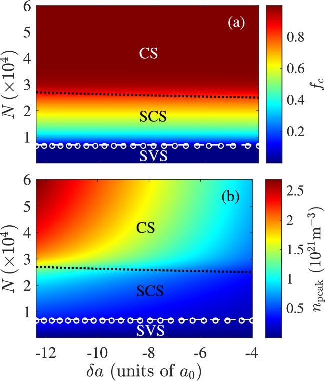
Figure 2. Distributions of the coherent fraction (a) and the peak density (b) on the δa-N parameter plane. The dashed line and ‘◦' denote, respectively, the analytically and numerically obtained boundaries between the SVS and SCS phases. The dotted lines mark the boundary between ${ \mathcal S }=1$ and 2. |
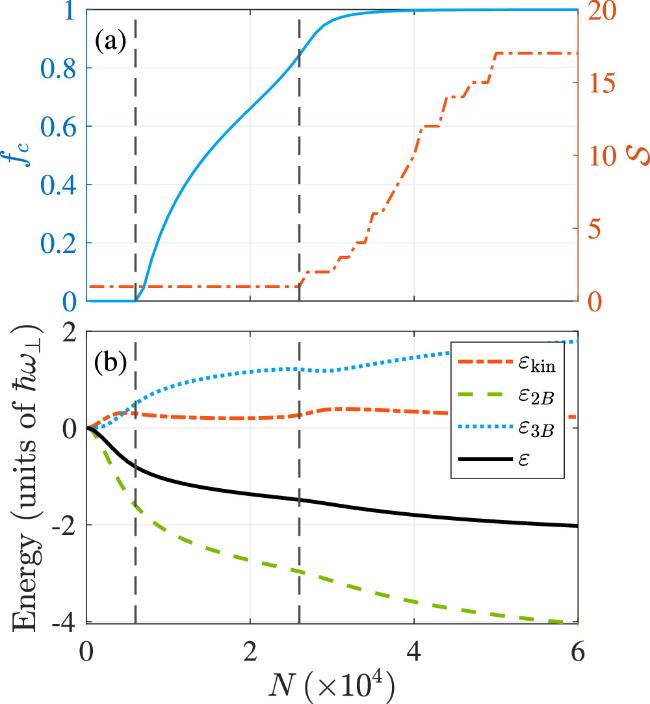
Figure 3. (a) fc versus N for δa = -11.78 a0. (b) N dependence of the ϵkin, ∣ϵ2B∣, ϵ3B, and ϵ with the same δa. The left vertical lines mark the boundary between SVS and SCS phases. The right vertical lines represent the boundary between ${ \mathcal S }=1$ and 2. |
To unveil more details on the quantum phases, we plot, in figure 3(a), the N dependence of fc and ${ \mathcal S }$ for N = 7000 and δa = − 11.78 a0. As can be seen, ${ \mathcal S }$ becomes larger than unit when N ≳ 2.6 × 10⁴. Furthermore, we plot the N dependence of the energy contributions ϵkin ≡ Ekin/N, ϵ2B ≡ E2B/N, ϵ3B ≡ E3B/N, and the total energy ϵ = ϵkin + ϵ2B + ϵ3B in figure 3(b). Here the correctness of the energy calculation is checked by the virial relation 2ϵkin + ϵ2B + 2ϵ3B = 0. Surprisingly, unlike the first-order transition from the SVS to SCS phases in quasi-2D binary droplets [39], ϵ and its derivatives does not have any discontinuity around the boundary between ${ \mathcal S }=1$ and 2. Therefore, the transition from the SVS to SCS phases is of a crossover type.
Interestingly, for the SVS-SCS transition, we may obtain an analytic condition for the transition boundary. To this end, we first introduce a fact found in numerical calculations. Namely, in the vicinity of the phase boundary, the normalized density profiles satisfy $\bar{n}(z)={\bar{n}}^{(s)}(z)={\bar{n}}^{(c)}(z)$. Then from equations (10 ) and (11 ), the 2B and 3B interaction energies can be evaluated as
$\begin{eqnarray}{E}_{2B}={\omega }_{2B}\left({N}^{(c)2}+6{N}^{(c)}{N}^{(s)}+3{N}^{(s)2}\right),\end{eqnarray}$
$\begin{eqnarray}\begin{array}{rcl}{E}_{3B} & = & {\omega }_{3B}\left({N}^{(c)3}+15{N}^{(c)2}{N}^{(s)}+45{N}^{(c)}{N}^{(s)2}\right.\\ & & \left.+15{N}^{(s)3}\right),\end{array}\end{eqnarray}$
where ${\omega }_{2B}=\delta g/(2\pi {a}_{\perp }^{2})\int {\rm{d}}z\bar{n}{\left(z\right)}^{2}$ with $\begin{eqnarray}\delta g=\displaystyle \frac{4\pi {{\hslash }}^{2}\delta a}{M}\displaystyle \frac{\sqrt{{a}_{\uparrow \uparrow }{a}_{\downarrow \downarrow }}}{{\left(\sqrt{{a}_{\uparrow \uparrow }}+\sqrt{{a}_{\downarrow \downarrow }}\right)}^{2}}\end{eqnarray}$
and ${\omega }_{3B}={g}_{3}^{\prime} /3!\int {\rm{d}}z\bar{n}{\left(z\right)}^{3}$. To proceed, let us assume that the system is at the SVS-SCS transition boundary with all for atoms in the SVS phase. As a result, the total energy $\begin{eqnarray}E(N)={\varepsilon }_{k}N+3{\omega }_{2B}{N}^{2}+15{\omega }_{3B}{N}^{3}.\end{eqnarray}$
Now if we add δN atoms into the system, the energy with δN atoms occupying the squeezed mode must be larger than that with δN atoms occupying the coherent mode. This observation then leads to the critical condition for the SVS-SCS transition, i.e. $\begin{eqnarray}-{E}_{2B}=3{E}_{3B},\end{eqnarray}$
which is numerically verified in figure 3(b).3.3. Axial width of the droplets
As the directly measurable quantities, the widths of the droplet are of great importance. In particular, for the radially trapped system, we are interested in droplet's axial width, i.e. ${\sigma }_{z}={\left[2{N}^{-1}\int {\rm{d}}{{zz}}^{2}n(z)\right]}^{1/2}$. Figure 2(a) plot the distribution of σz on the δa-N plane. As can be seen, the typical value of σz is several micrometers, which confirms that the axial size is experimentally accessible through in situ measurement. In addition, nontrivial structures also developed in figure 2(a), in analogy to that observed in the two-dimensional binary droplets [39].
To gain more sight into the droplet's axial width, we plot, in figure 4(b), the numerically obtained σz as a function of N (solid line) for δa = -11.78 a0. In accordance with the structure in figure 2(a), the σz-N curve is of the W shape. Following [39], we analyze σz using a simple variational method. To this end, we note that, quite generally, the total energy per atom, ε ≡ E/N, can be expressed as29 ), one finds the equilibrium axial width,
$\begin{eqnarray}\epsilon ({w}_{z})\propto \displaystyle \frac{1}{{w}_{z}^{2}}+\displaystyle \frac{{\tilde{g}}_{2}N}{{w}_{z}}+\displaystyle \frac{{\tilde{g}}_{3}{N}^{2}}{{w}_{z}^{2}},\end{eqnarray}$
where wz is the width along the axial direction and ${\tilde{g}}_{2}$ (<0) and ${\tilde{g}}_{3}$ (>0) are two reduced strengths associated with the two- and three-body interactions, respectively. Clearly, ${\tilde{g}}_{2}$ (<0) and ${\tilde{g}}_{3}$ depend on the density profile of the droplets. Then by minimizing equation ( $\begin{eqnarray}{\sigma }_{z}(N)=\displaystyle \frac{2{\tilde{g}}_{3}{N}^{2}+2}{-{\tilde{g}}_{2}N}.\end{eqnarray}$
Apparently, σz(N) goes to ∞ for both limits N → 0 and ∞. In addition, σz(N) is minimum at $N={\tilde{g}}_{3}^{-1/2}$. Therefore, σ(N) is always a V-shaped curve. Interestingly, the critical atom number is zero for the quasi-1D droplets, indicating that, in the presence of attractive interaction, a self-bound state always forms for 1D geometry.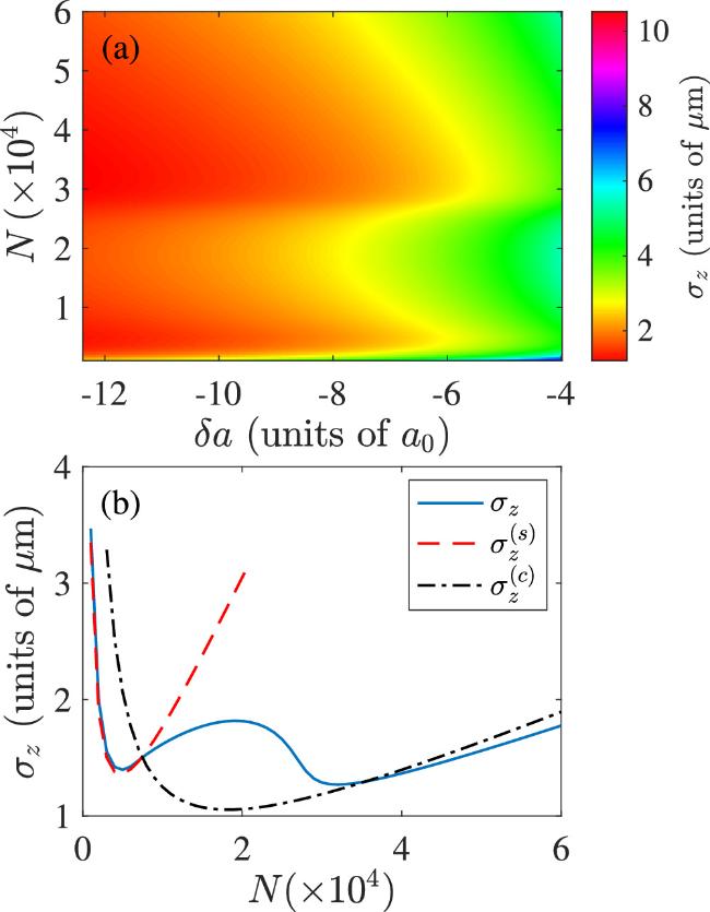
Figure 4. (a) Distribution of the axial size on the δa-N parameter plane. (b)The dashed lines denote the boundary between the SVS and SCS phases. |
To make quantitative comparisons between the variational and numerical results, we assume that all density profiles are proportional to a Gaussian function30 ) using the reduced interaction parameters $\left({\tilde{g}}_{2}^{(c)},{\tilde{g}}_{3}^{(c)}\right)$ and $\left({\tilde{g}}_{2}^{(s)},{\tilde{g}}_{3}^{(s)}\right)$, respectively. As can be seen, ${\sigma }_{z}^{(s)}$ agrees very well with σz around the left dip where the condensate is a SVS. This agreement is supported by the fact that the density profile of a SVS is well approximated by Gaussian functions. Around the right dip, the quantum state of the condensate is a SCS, instead of a pure coherent state. Therefore, ${\sigma }_{z}^{(c)}$ only exhibits a rough agreement with ${\sigma }_{z}^{(\mathrm{GST})}$ for large N where the quantum state is dominated by coherent component. In addition, the density profile of the coherent state is significantly deviated from a Gaussian function in the strong interaction regime, which leads to more discrepancy. Nevertheless, similar to that in the 2D binary droplets [39], the W-shaped σz-N curve provides a strong evidence for the multiple quantum phases emerged in the self-bound droplets.
$\begin{eqnarray}\bar{n}(z)=\frac{1}{{\pi }^{1/2}{w}_{z}}{{\rm{e}}}^{-{z}^{2}/{w}_{z}^{2}}.\end{eqnarray}$
Then for the CS and SVS states, we obtain two sets of reduced interaction strengths $\left({\tilde{g}}_{2}^{(c)},{\tilde{g}}_{3}^{(c)}\right)$ and $\left({\tilde{g}}_{2}^{(s)},{\tilde{g}}_{3}^{(s)}\right)$, respectively, where ${\tilde{g}}_{2}^{(c)}=4\delta g/[{\left(2\pi \right)}^{3/2}{a}_{\perp }^{2}]$, ${\tilde{g}}_{3}^{(c)}=32{g}_{3}/(9\pi \sqrt{3}{a}_{\perp }^{4})$, ${\tilde{g}}_{2}^{(s)}\,=3{\tilde{g}}_{2}^{(c)}$, and ${\tilde{g}}_{3}^{(s)}=15{\tilde{g}}_{c}^{(c)}$. In figure 2(b), the dashed and dash-dotted lines are the plots of equation (Interestingly, using these reduced interaction parameters, we may analytically derive from equation (28 ) that the SVS-SCS transition occurs at $N=2/{\tilde{g}}_{3}^{(s)}$. As shown in figure 2, this analytic critical condition is very good agreement with the numerical results.
4. Dynamical generation of macroscopic squeezing
Here we study the dynamical generation of macroscopic squeezing by tuning the scattering lengths. For the Feshbach resonance used in the experiment [9], a↑↑ and a↑↓ are barely changed. Therefore, we shall only allow a↓↓ to vary in our simulations. Specifically, the scattering length a↓↓ is swept by following the function32 ).
$\begin{eqnarray}{a}_{\downarrow \downarrow }(t)={a}_{i}{{\rm{e}}}^{-{rt}/{\tau }_{s}},\end{eqnarray}$
where ai is the initial scattering length, τs is the sweeping time, and $r=\mathrm{ln}({a}_{i}/{a}_{f})$ with af being the final scattering length. We point out that although other function forms for a↓↓(t) have also been tried for a given set of (ai, af, τs), only quantitative differences on the macroscopic squeezing are found. Consequently, we shall only present the simulation results using the sweeping function equation (Our numerical simulations start with a ground state wave function under the magnetic field B = 56.86 G with various atom number N's. Correspondingly, the initial scattering length is ai = 85.1a0 which gives rise to a positive reduced scattering length δai = 0.04a0. As a result, the condensate is initially in a coherent state. To efficiently generate macroscopic squeezing, the target scattering length af is so chosen that the final reduced scattering length is negative, i.e. δaf < 0. Finally, it should be note that, unlike the self-bound ground states, the atomic gas may significantly expand along the axial direction, which poses an effective challenge to numerical simulations. To circumvent this difficulty, we introduce a harmonic confinement along the z direction with frequency ωz/(2π) = 102 Hz. Accordingly, to make the quasi-1D assumption still hold, we radial trap frequency is increased to ω⊥/(2π) = 103 Hz.
Figure 5 present the main results for the dynamical generating of the macroscopic squeezing. The general observation is that, by simply tuning the scattering length, a large fraction of coherent atoms are transferred into the macroscopic squeezing, which is in striking contrast to the single component case [40]. Specifically, we compare, in figure 5(a), the relative macroscopic squeezing corresponding to different sweeping times. As can be seen, different τs's give rise to similar dynamical behavior such that the largest ${N}_{1}^{(s)}/N$'s achieved in simulations are also close to each other. We can therefore say that the dynamics is rather insensitive to the variation of the sweeping time. In figure 5(b), we further compare ${N}_{1}^{(s)}(t)/N$'s corresponding to different total atom numbers, which unsurprisingly shows that larger N leads to larger ${N}_{1}^{(s)}/N$. The underlying reason is clearly due to that the attractive interaction is enhanced by higher density. For the similar reason, it is seen from figure 5(c) that smaller af (equivalently, larger ∣δaf∣) generates more macroscopic squeezing. Particularly, the largest ${N}_{1}^{(s)}/N$ for each simulations is rather sensitive to af.
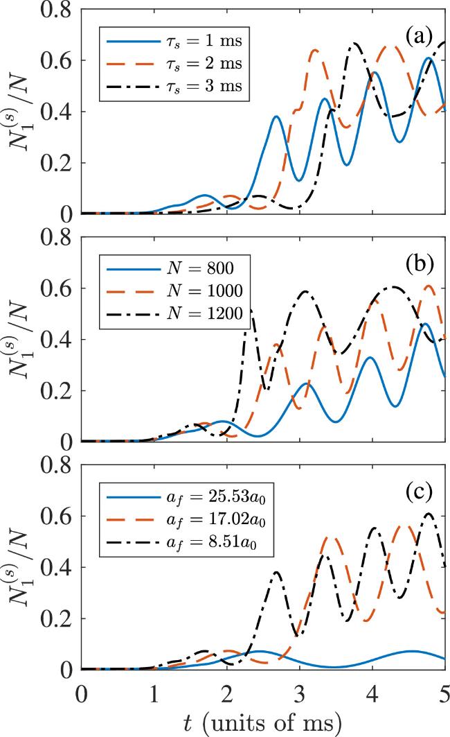
Figure 5. ${N}_{1}^{(s)}/N$ versus t for (a) different sweeping times with N = 103 and af = 8.51 a0; (b) different atom numbers with τs = 1 ms and af = 8.51 a0; (c) different target scattering lengths with N = 103 and τs = 1 ms. |
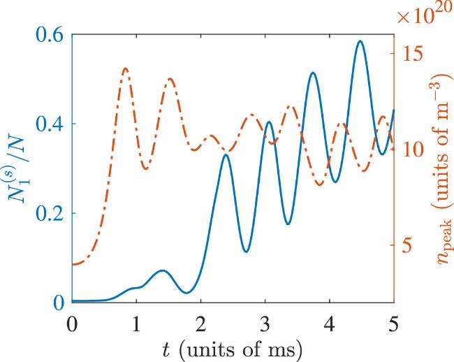
To gain more insight into the origin of the macroscopic squeezing, we plot, in figure 6, the quench dynamics of the fraction of the macroscopic squeezing ${N}_{1}^{(s)}/N$ and the peak condensate density npeak. As can be seen, for the initial stage of the dynamics (t ≲ 2 ms), ${N}_{1}^{(s)}/N$ is peaked at roughly the local maximum of npeak, which suggests that the macroscopic squeezing is generated when condensate shrinks due to the attractive interaction. However, this observation does not hold for the long-time dynamics. In fact, for large t, multiple peaks may develop in the density profile, among which the lower peaks may contribute significantly to the macroscopic squeezing. Consequently, the dynamics of ${N}_{1}^{(s)}/N$ becomes out of synchronization to that of npeak.
Figure 6. Quench dynamics of ${N}_{1}^{(s)}/N$ (solid line) and npeak (dash-dotted line) for N = 103 and af = 8.51 a0. |
5. Conclusion
In summary, we have systematically studied the ground-state properties and the dynamics of a quasi-1D binary Bose condensates using the Gaussian state theory. For the ground states of the droplets, we have found that three distinct quantum phases, including SVS, SCS, and CS. In particular, it was found that the transition between the SCS and CS phases is of a crossover type, in striking contrast to the first order transition in quasi-2D binary droplets. As to the dynamics, we show that up to 60% of the total atom can be converted from a coherent state to the macroscopic squeezed state by tuning the reduced scattering length to a negative value, which suggests that macroscopic squeezing can be more efficiently generated in two-component condensates as compared to the single-component ones.