


1. Introduction
2. Inverse scattering transform
2.1. Spectral analysis
Let ${q}_{0}\in \tanh (x)+{L}^{1}({\mathbb{R}})$ and $q{{\prime} }_{0}\in {W}^{\mathrm{1,1}}({\mathbb{R}})$, then we have
| i | (i) ${\phi }_{1}^{+}(z)$ and ${\phi }_{2}^{-}(z)$ can be analytically extended to $z\in {{\mathbb{C}}}^{-}$, while ${\phi }_{1}^{-}(z)$ and ${\phi }_{2}^{+}(z)$ can be analytically extended to $z\in {{\mathbb{C}}}^{+}$. |
| ii | (ii) ${\phi }^{\pm }(z)$ satisfy the symmetries $\begin{eqnarray}{\phi }^{\pm }(z)={\sigma }_{1}\overline{{\phi }^{\pm }(\bar{z})}{\sigma }_{1}=\pm {z}^{-1}{\phi }^{\pm }({z}^{-1}){\sigma }_{1}.\end{eqnarray}$ |
| iii | (iii) ${\phi }^{\pm }(z)$ admit the asymptotic properties $\begin{eqnarray*}\begin{array}{rcl}{\phi }^{\pm }(z) & = & {{\rm{e}}}^{{\rm{i}}\beta {\displaystyle \int }_{\pm \infty }^{x}(| q{| }^{2}-1){\rm{d}}y{\sigma }_{3}}+{ \mathcal O }\left({z}^{-1}\right),\ z\to \infty ,\\ {\phi }^{\pm }(z) & = & -{\rm{i}}{z}^{-1}{\sigma }_{1}{{\rm{e}}}^{{\rm{i}}\beta {\displaystyle \int }_{\pm \infty }^{x}(| q{| }^{2}-1){\rm{d}}y}+{ \mathcal O }(1),\ z\to 0.\end{array}\end{eqnarray*}$ |
Let ${q}_{0}\in \tanh x+{H}^{\mathrm{2,2}}({\mathbb{R}})$, then
| i | (i)The scattering data a(z) can be analytically extended to $z\in {{\mathbb{C}}}^{+}$, while b(z) is defined for $z\in {\mathbb{R}}\setminus \{0,\pm 1\}$. Zeros of a(z) in ${{\mathbb{C}}}^{+}$ are simple, finite and distribute on the unit circle. |
| ii | (ii) $a(z)=a({z}^{-1})$ , $b(z)=-b({z}^{-1}),$ $r(z)=-r({z}^{-1}).$ |
| iii | (iii)The scattering data admit asymptotics $\begin{eqnarray*}| b(z)| ={ \mathcal O }(| z{| }^{-2}),\ | z| \to \infty ,\ | b(z)| ={ \mathcal O }(| z{| }^{2}),\ | z| \to 0.\end{eqnarray*}$ |
| iv | (iv)In the non-generic case, a(z) and $b(z)$ are continuous at $z=\pm 1$ and $| r(\pm 1)| \lt 1;$ In the generic case, a(z) and b(z) have the first order singularities at $z=\pm 1$, $\begin{eqnarray}a(z)=\displaystyle \frac{{c}_{\pm }}{z\mp 1}+{ \mathcal O }(1),\ b(z)=\mp \displaystyle \frac{{c}_{\pm }}{z\mp 1}+{ \mathcal O }(1),\end{eqnarray}$ which leads to ${\mathrm{lim}}_{z\to \pm 1}r(z)=\mp 1$, where ${c}_{\pm }\,=\det \left[{\psi }_{1}^{-}(\pm 1),{\psi }_{2}^{+}(\pm 1)\right].$ |
2.2. Set-up of the RH problem
Find a matrix-valued function M(z) which satisfies
| 1.Analyticity: M(z) is meromorphic in ${\mathbb{C}}\setminus {\mathbb{R}}$. | |
| 2.Jump condition: M(z) satisfies the jump condition $\begin{eqnarray*}\begin{array}{l}{M}_{+}(z)={M}_{-}(z)V(z),\ z\in {\mathbb{R}},\end{array}\end{eqnarray*}$ where $\begin{eqnarray}V(z)=\left(\begin{array}{cc}1-| r(z){| }^{2} & -\overline{r(z)}{{\rm{e}}}^{-2{\rm{i}}t\theta (z)}\\ r(z){{\rm{e}}}^{2{\rm{i}}t\theta (z)} & 1\end{array}\right),\end{eqnarray}$ with $\theta (z)=\zeta (z)\tfrac{x}{t}-2\zeta (z)\lambda (z).$ | |
| 3.Asymptotic behaviors: $\begin{eqnarray*}\begin{array}{rcl}M(z) & = & I+{ \mathcal O }({z}^{-1}),\quad z\to \infty ,\\ {zM}(z) & = & {\sigma }_{1}+{ \mathcal O }(z),\quad z\to 0.\end{array}\end{eqnarray*}$ | |
| 4.Residue conditions: M(z) has simple poles at each points zj in ${{ \mathcal Z }}^{+}\cup {{ \mathcal Z }}^{-}$ with the following residue conditions: $\begin{eqnarray}\mathop{\mathrm{Res}}\limits_{z={z}_{j}}M(z)=\mathop{\mathrm{lim}}\limits_{z\to {z}_{j}}M(z)\left(\begin{array}{cc}0 & 0\\ {c}_{j}{{\rm{e}}}^{2{\rm{i}}t\theta ({z}_{j})} & 0\end{array}\right),\end{eqnarray}$ $\begin{eqnarray}\mathop{\mathrm{Res}}\limits_{z={\bar{z}}_{j}}M(z)=\mathop{\mathrm{lim}}\limits_{z\to {\bar{z}}_{j}}M(z)\left(\begin{array}{cc}0 & {\bar{c}}_{j}{{\rm{e}}}^{-2{\rm{i}}t\theta ({\bar{z}}_{j})}\\ 0 & 0\end{array}\right),\end{eqnarray}$ where ${c}_{j}=\tfrac{4{\rm{i}}{z}_{j}}{{\int }_{{\mathbb{R}}}| {\psi }_{2}^{+}({z}_{j};x,0){| }^{2}{\rm{d}}x}={\rm{i}}{z}_{j}| {c}_{j}| .$ |

Figure 1. The poles and jump lines of M(z). |
2.3. Classification of asymptotic regions
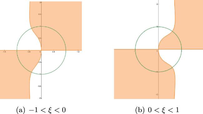
Figure 2. Solitonic regions: ∣ξ∣ < 1, there is no phase point on ${\mathbb{R}}$. |
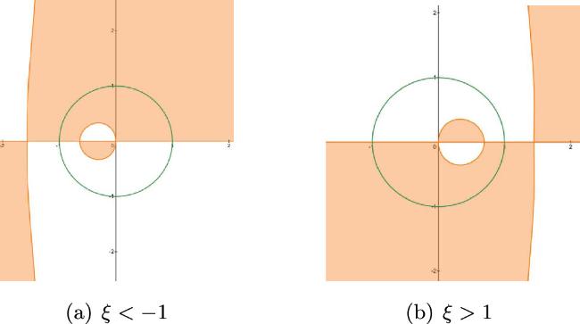
Figure 3. Solitonless region: ∣ξ∣ > 1, there are two phase points on ${\mathbb{R}}$. |
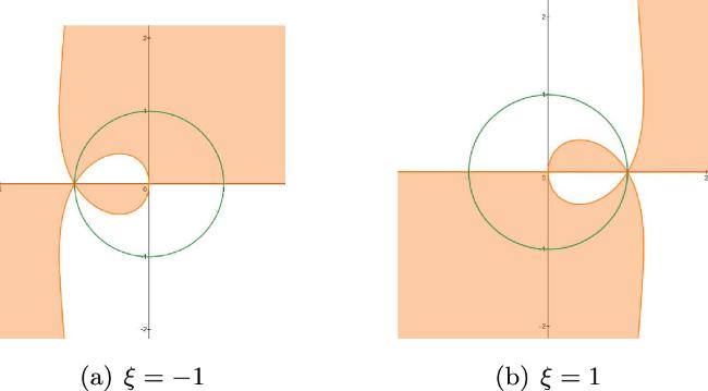
Figure 4. Transition region: ∣ξ∣ = 1, there is one phase point on ${\mathbb{R}}$. |
3. Long-time asymptotic behavior
3.1. Solitonic region
The initial data ${q}_{0}\in \tanh (x)+{H}^{\mathrm{4,4}}({\mathbb{R}})$, and $\{r(z),{\{{z}_{j},{c}_{j}\}}_{j\,=\,0}^{N-1}\}$ are associated with the scattering data. Then in the solitonic region $| x/(2t)| \lt 1$, the N-soliton solution of the Cauchy problem (
3.2. Solitonless region
Under the condition of the theorem
3.3. Two transition regions
The initial data given in theorem
| 1.In the transition region ${{ \mathcal A }}_{-1}$, the solution to the Cauchy problem ( $\begin{eqnarray}\begin{array}{rcl}q(x,t) & = & 2{\rm{i}}m(x,t){{\rm{e}}}^{4{\rm{i}}\beta {\displaystyle \int }_{\infty }^{x}(| m(y,t){| }^{2}-1){\rm{d}}y},\\ m(x,t) & = & {{\rm{e}}}^{{\rm{i}}\varepsilon }\left(1+{\left(\displaystyle \frac{3}{4}t\right)}^{-1/3}\alpha (-1)\right)+{ \mathcal O }\left({t}^{-1/2}\right),\end{array}\end{eqnarray}$ where $\varepsilon $ and $\alpha (-1)$ are the associated parameters $\begin{eqnarray}\begin{array}{l}\varepsilon =\displaystyle \frac{1}{2\pi }{\displaystyle \int }_{0}^{\infty }\displaystyle \frac{\mathrm{log}(1-| r(z){| }^{2})}{z}\,{\rm{d}}z+2\displaystyle \sum _{j=0}^{N-1}\arg {z}_{j},\\ \alpha (-1)=\displaystyle \frac{{\rm{i}}}{2}\left({\displaystyle \int }_{s}^{\infty }{u}^{2}(y){\rm{d}}y-u(s){{\rm{e}}}^{\mathrm{iarg}(r(-1)}\right),\\ \,s=\displaystyle \frac{8}{3}\left(\displaystyle \frac{x}{2t}+1\right){\left(\displaystyle \frac{3}{4}t\right)}^{\tfrac{2}{3}},\end{array}\end{eqnarray}$ and $u(s)$ is the solution of the Painlevé equation $\begin{eqnarray}u^{\prime\prime} (s)=2{u}^{3}(s)+{su}(s).\end{eqnarray}$ | |
| 2.In the transition region ${{ \mathcal A }}_{+1}$, the solution to the Cauchy problem ( $\begin{eqnarray}\begin{array}{rcl}q(x,t) & = & 2{\rm{i}}m(x,t){{\rm{e}}}^{4{\rm{i}}\beta {\displaystyle \int }_{\infty }^{x}(| m(y,t){| }^{2}-1){\rm{d}}y},\\ m(x,t) & = & {{\rm{e}}}^{{\rm{i}}\varepsilon }\left(1+{\left(\displaystyle \frac{3}{4}t\right)}^{-1/3}\alpha (1)\right)+{ \mathcal O }\left({t}^{-1/2}\right),\end{array}\end{eqnarray}$ where $\begin{eqnarray}\begin{array}{rcl}\varepsilon & = & \displaystyle \frac{1}{2\pi }{\displaystyle \int }_{0}^{\infty }\displaystyle \frac{\mathrm{log}(1-| r(z){| }^{2})}{z}\,{\rm{d}}z,\\ \alpha (1) & = & -\displaystyle \frac{{\rm{i}}}{2}\left({\displaystyle \int }_{s}^{\infty }{u}^{2}(y){\rm{d}}y-u(s){{\rm{e}}}^{\mathrm{iarg}(\overline{\tilde{r}(1)})}\right),\\ s & = & -\displaystyle \frac{8}{3}(\displaystyle \frac{x}{2t}-1){\left(\displaystyle \frac{3}{4}t\right)}^{\tfrac{2}{3}},\end{array}\end{eqnarray}$ and $u(s)$ is a real-value solution of the Painevé equation ( |