Welcome to visit Communications in Theoretical Physics,
Mathematical Physics

On limit fractional Volterra hierarchies

  • Lixiang Zhang 1 ,
  • Chuanzhong Li 1, 2, *
Expand
  • 1School of Mathematics and Statistics, Ningbo University, Ningbo, 315211, China
  • 2College of Mathematics and Systems Science, Shandong University of Science and Technology, Qingdao, 266590, China

Author to whom any correspondence should be addressed.

Received date: 2023-02-04

  Revised date: 2023-11-06

  Accepted date: 2023-11-08

  Online published: 2024-01-19

Copyright

© 2024 Institute of Theoretical Physics CAS, Chinese Physical Society and IOP Publishing

Abstract

For the limit fractional Volterra (LFV) hierarchy, we construct the n-fold Darboux transformation and the soliton solutions. Furthermore, we extend the LFV hierarchy to the noncommutative LFV (NCLFV) hierarchy, and construct the Darboux transformation expressed by quasi determinant of the noncommutative version. Meanwhile, we establish the relationship between new and old solutions of the NCLFV hierarchy. Finally, the quasi determinant solutions of the NCLFV hierarchy are obtained.

Cite this article

Lixiang Zhang , Chuanzhong Li . On limit fractional Volterra hierarchies[J]. Communications in Theoretical Physics, 2024 , 76(1) : 015002 . DOI: 10.1088/1572-9494/ad0a6d

1. Introduction

The 2D Toda lattice hierarchy [1, 2] is one of the most fundamental topics in the theory of integrable systems. This hierarchy is a completely integrable system, which has many important applications in mathematics and physics including the representation theory of Lie algebras, orthogonal polynomials, random matrix models [36], and the theory of Gromov-Witten invariants [7]. Many known integrable nonlinear partial differential and difference equations are reductions or special cases of 2D Toda lattice. For example, the 1D Toda hierarchy [810], interestingly, the topological sigma model (geometrically, the Gromov-Witten invariants) of the Riemann sphere CP1, which is related to the 1D Toda hierarchy, the Ablowitz-Ladik hierarchy [11], which can control the Gromov-Witten theory [12], the fractional Volterra (FV) hierarchy [13] and the multi-component extension version of this hierarchy [14], and the limit fractional Volterra (LFV) hierarchy [15], which can control the linear Hodge integral. Particularly, the LFV hierarchy is a new system defined by Liu in 2021 [15], which can be as a certain reduction of the 2D Toda hierarchy. Moreover, the reduced equations can be further reduced to finite-dimensional systems like Newton equations for a system of particles, Garnier system and other models [16].
There are many good properties of the LFV hierarchy, such as it's a tau-symmetric Hamiltonian integrable hierarchy, and it contains two sub-hierarchies: the intermediate long wave hierarchy (ILW) [17] and the limit of the FV hierarchy [18]. It is proved by Buryak in [17, 19] that the Hodge hierarchy for linear Hodge integrals is equivalent to the ILW hierarchy, and the relationship between the LFV hierarchy and the ILW hierarchy is established by the Miura-type transformation, the equations of the flows t1,n in the LFV hierarchy are transformed to the symmetries of the ILW hierarchy. In other words, the LFV hierarchy can be an extension of the ILW hierarchy. The FV hierarchy is an integrable hierarchy, which can be regarded as a fractional generalization of the Volterra lattice hierarchy [20], and which is also regarded as a reduction of the bigraded Toda hierarchy [21, 22]. Liu [18] gave the definition of this integrable hierarchy in terms of Lax pair and Hamiltonian formalisms, and he presented its tau functions and multi-soliton solutions. Moreover, the generating function of cubic Hodge integrals satisfies the local Calabi-Yau condition, which is conjectured to be a tau function of the FV hierarchy.
Based on the excellent properties of the LFV hierarchy, we want to explore its other properties. It was pointed out that the Darboux transformation was an efficient method to generate soliton solutions of integrable equations. The multi-solitons can be obtained by this Darboux transformation from a trivial seed solution. If we give the Lax pair of this hierarchy, on this basis, we can construct the Darboux transformation and obtain the soliton solutions using the Darboux transformation of the LFV hierarchy. Further, we want to extend this hierarchy to the noncommutative version [2325].
Figure 1. When parameters are p = 2, λ1 = 1 and ϵ = 0.5, u[1] is the soliton solution.
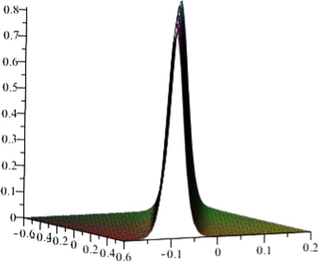
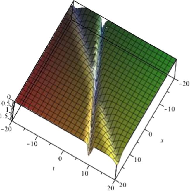
Figure 2. When parameters are p = 2, λ1 = 1, λ2 = 2 and ϵ = 0.5, u[2] is the two-soliton solution.
This paper is arranged as follows: In section 2, summarizing the related lemmas and definition of the LFV hierarchy, we construct the Darboux transformation [22, 26] of the LFV hierarchy, and obtain the corresponding relationship between the old and new solutions. Furthermore, the one and two soliton solutions are obtained from the LFV hierarchy. In section 3, we extend the LFV hierarchy to the NCLFV hierarchy. And we construct the Darboux transformation of the noncommutative version [27, 28]. Meanwhile, we obtain the quasi determinant [29] solution of the NCLFV hierarchy. Finally, we draw a brief conclusion of this paper.

2. The LFV hierarchy

2.1. The definition of the LFV hierarchy

We recall the two Lax operators of 2D Toda hierarchy
$\begin{eqnarray}L={\rm{\Lambda }}+{a}_{0}+{a}_{1}{{\rm{\Lambda }}}^{-1}+\cdots ,\end{eqnarray}$
$\begin{eqnarray}\bar{L}={{\rm{e}}}^{u}{{\rm{\Lambda }}}^{-1}+{b}_{0}+{b}_{1}{\rm{\Lambda }}+\cdots ,\end{eqnarray}$
where Λ represents shift operator ${\rm{\Lambda }}:= {{\rm{e}}}^{\epsilon {\partial }_{x}}$, which acts on the function f(x) with one variable x, Λnf(x) = f(x + nε), and ai = ai(u), bi = bi(u) for i ≥ 0. The Lax operators (2.1) and (2.2) can be written as the dressing operators
$\begin{eqnarray}L=P{\rm{\Lambda }}{P}^{-1},\,P=1+\displaystyle \sum _{k\geqslant 1}{p}_{k}{{\rm{\Lambda }}}^{-k},\end{eqnarray}$
$\begin{eqnarray}\bar{L}=Q{{\rm{\Lambda }}}^{-1}{Q}^{-1},\,Q=\displaystyle \sum _{k\geqslant 0}{q}_{k}{{\rm{\Lambda }}}^{k}.\end{eqnarray}$
The logarithm of the operators (2.1) and (2.2) is defined by
$\begin{eqnarray*}\begin{array}{l}\mathrm{log}L:= P(\varepsilon {\partial }_{x}){P}^{-1}=\varepsilon {\partial }_{x}-\varepsilon {P}_{x}{P}^{-1},\\ \mathrm{log}\bar{L}:= Q(-\varepsilon {\partial }_{x}){Q}^{-1}=-\varepsilon {\partial }_{x}+\varepsilon {Q}_{x}{Q}^{-1},\end{array}\end{eqnarray*}$
where Px = ∑k≥1(∂xpkk and Qx = ∑k≥0(∂xqkk.

([15]) There exist differential polynomials ak such that

$\begin{eqnarray*}\mathop{\mathrm{lim}}\limits_{\varepsilon \to 0}{a}_{k}=\displaystyle \frac{{p}^{k+1}}{(k+1)!}{{\rm{e}}}^{(k+1)u},\end{eqnarray*}$
and the difference operator L in (2.1) satisfies
$\begin{eqnarray*}\displaystyle \frac{1}{p}\mathrm{log}L=K,\end{eqnarray*}$
where K is a differential-difference operator, which is defined by
$\begin{eqnarray}K=\displaystyle \frac{1}{p}\epsilon {\partial }_{x}+{{\rm{e}}}^{u}{{\rm{\Lambda }}}^{-1}.\end{eqnarray}$
Meanwhile, the expression of ai in (2.1) can be obtained, the recurrence relations are
$\begin{eqnarray}\displaystyle \frac{1}{p}\epsilon {\partial }_{x}{a}_{i+1}={a}_{k}{{\rm{\Lambda }}}^{-k}{{\rm{e}}}^{u}-{{\rm{e}}}^{u}{{\rm{\Lambda }}}^{-1}{a}_{i},\,i\geqslant 0,\end{eqnarray}$
with
$\begin{eqnarray}{a}_{0}=p\displaystyle \frac{{\rm{\Lambda }}-1}{\epsilon {\partial }_{x}}{{\rm{e}}}^{u}.\end{eqnarray}$

([15]) There exist unique differential polynomials bk such that

$\begin{eqnarray*}\mathop{\mathrm{lim}}\limits_{\varepsilon \to 0}{b}_{k}=\displaystyle \frac{{{\rm{e}}}^{-{ku}}}{{p}^{k+1}}{\beta }_{k},\end{eqnarray*}$
and the difference operator $\bar{L}$ in (2.2) satisfies
$\begin{eqnarray*}\bar{L}-\displaystyle \frac{1}{p}\mathrm{log}\bar{L}=K,\end{eqnarray*}$
where K is defined by (2.5), and bk satisfies the following recursion relations
$\begin{eqnarray}\begin{array}{l}\displaystyle \frac{1}{p}\epsilon {\partial }_{x}{b}_{k}={b}_{k+1}{{\rm{\Lambda }}}^{k+1}{{\rm{e}}}^{u}-{{\rm{e}}}^{u}{{\rm{\Lambda }}}^{-1}{b}_{k+1},\\ \,k\geqslant -1,\end{array}\end{eqnarray}$
with ${b}_{-1}={{\rm{e}}}^{u}$.

The LFV hierarchy consists of the flows

$\begin{eqnarray}\begin{array}{l}\varepsilon \displaystyle \frac{\partial K}{\partial {t}_{1,n}}=[{\left({L}^{n}\right)}_{+},K],\\ \varepsilon \displaystyle \frac{\partial K}{\partial {t}_{2,n}}=-[{\left({\bar{L}}^{n}\right)}_{-},K],\,n\geqslant 1,\end{array}\end{eqnarray}$
where K is defined by (2.5), L is determined by (2.1) and satisfies the conditions in lemma 1, $\bar{L}$ is determined by (2.2) and satisfies the conditions in lemma 2. For $A={\sum }_{i\in Z}{a}_{i}(x){{\rm{\Lambda }}}^{i}$, ${A}_{+}={\sum }_{i\geqslant 0}{a}_{i}(x){{\rm{\Lambda }}}^{i}$, ${A}_{-}={\sum }_{i\lt 0}{a}_{i}(x){{\rm{\Lambda }}}^{i}$.

When n = 1, the equations of ${t}_{\mathrm{1,1}}$ and ${t}_{2.1}$ flows of the LFV hierarchy respectively are

$\begin{eqnarray}\displaystyle \frac{\partial u}{\partial {t}_{\mathrm{1,1}}}=p\displaystyle \frac{(1-{{\rm{\Lambda }}}^{-1})({\rm{\Lambda }}-1)}{{\varepsilon }^{2}{\partial }_{x}}{{\rm{e}}}^{u},\end{eqnarray}$
$\begin{eqnarray}\displaystyle \frac{\partial u}{\partial {t}_{\mathrm{2,1}}}=\displaystyle \frac{1}{p}{u}_{x}.\end{eqnarray}$

Meanwhile, the operators L and $\bar{L}$ satisfy the Lax equations
$\begin{eqnarray}\varepsilon \displaystyle \frac{\partial L}{\partial {t}_{1,n}}=[{\left({L}^{n}\right)}_{+},L],\,\varepsilon \displaystyle \frac{\partial L}{\partial {t}_{2,n}}=[-{\left({\bar{L}}^{n}\right)}_{-},L];\end{eqnarray}$
$\begin{eqnarray}\varepsilon \displaystyle \frac{\partial \bar{L}}{\partial {t}_{1,n}}=[{\left({L}^{n}\right)}_{+},\bar{L}],\,\varepsilon \displaystyle \frac{\partial \bar{L}}{\partial {t}_{2,n}}=[-{\left({\bar{L}}^{n}\right)}_{-},\bar{L}].\end{eqnarray}$

Actually, the LFV hierarchy (2.9) can be also equivalently rewritten as the linear differential equations

$\begin{eqnarray}\left\{\begin{array}{l}K\phi =\lambda \phi ,\\ \varepsilon \displaystyle \frac{\partial \phi }{\partial {t}_{1,n}}={\left({L}^{n}\right)}_{+}\phi ,\end{array}\right.\end{eqnarray}$
$\begin{eqnarray}\left\{\begin{array}{l}K\phi =\lambda \phi ,\\ \varepsilon \displaystyle \frac{\partial \phi }{\partial {t}_{2,n}}=-{\left({\bar{L}}^{n}\right)}_{-}\phi ,\end{array}\right.\end{eqnarray}$
where λ is a parameter, and $\phi =\phi (x,t)$ is the wave function of the LFV hierarchy (2.9).

For the first equation of (2.14a), taking the derivative about variable ${t}_{1,n}$ of both sides of it, we have

$\begin{eqnarray}{K}_{{t}_{1,n}}\phi +K{\phi }_{{t}_{1,n}}=\lambda {\phi }_{{t}_{1,n}}.\end{eqnarray}$
Substituting the second equation of (2.14a) into equation (2.15), we have
$\begin{eqnarray}\begin{array}{l}{K}_{{t}_{1,n}}\phi +\displaystyle \frac{1}{\varepsilon }K{\left({L}^{n}\right)}_{+}\phi =\lambda {\phi }_{{t}_{1,n}}{\left({L}^{n}\right)}_{+}\phi \\ \,=\,\displaystyle \frac{1}{\varepsilon }{\left({L}^{n}\right)}_{+}K\phi ,\end{array}\end{eqnarray}$
thus
$\begin{eqnarray}\begin{array}{l}\varepsilon {K}_{{t}_{1,n}}={\left({L}^{n}\right)}_{+}K-K{\left({L}^{n}\right)}_{+}\\ \,=\,[{\left({L}^{n}\right)}_{+},K].\end{array}\end{eqnarray}$
Using the similar calculation method, we can prove that the linear equations (2.14b) are the equivalent form of ${t}_{2,n}$ flow equations in the LFV hierarchy. □

2.2. Darboux transformation of the LFV hierarchy

In this section, we construct the n-fold Darboux transformation of the LFV hierarchy, and obtain the relationship between new and old solutions.
We consider the Darboux transformation of the LFV hierarchy on Lax operator K in (2.5), let
$\begin{eqnarray}{K}^{[1]}=\displaystyle \frac{1}{p}\varepsilon {\partial }_{x}+{{\rm{e}}}^{{u}^{[1]}}{{\rm{\Lambda }}}^{-1}={{TKT}}^{-1},\end{eqnarray}$
where T is the Darboux transformation operator. In order to keep the Lax equations (2.9) invariant, we have
$\begin{eqnarray}\begin{array}{l}\varepsilon \displaystyle \frac{\partial {K}^{[1]}}{\partial {t}_{1,n}}=[{\left({\left({L}^{[1]}\right)}^{n}\right)}_{+},K],\\ \varepsilon \displaystyle \frac{\partial {K}^{[1]}}{\partial {t}_{2,n}}=-[{\left({\left({\bar{L}}^{[1]}\right)}^{n}\right)}_{-},K],\,n\geqslant 1,\end{array}\end{eqnarray}$
where L[1] = TLT−1 and ${\bar{L}}^{[1]}=T\bar{L}{T}^{-1}$.

The Darboux transformation operator T should satisfy the following equations

$\begin{eqnarray}\varepsilon {T}_{{t}_{q,n}}=-T{\left({L}_{q}^{n}\right)}_{+}+{\left({{TL}}_{q}^{n}{T}^{-1}\right)}_{+}T,\,q=1,2,\,n\geqslant 1,\end{eqnarray}$
where ${L}_{1}=L$, ${L}_{2}=\bar{L}$.

From (2.18),

$\begin{eqnarray*}\begin{array}{l}\varepsilon \displaystyle \frac{\partial {K}^{[1]}}{\partial {t}_{q,n}}=\varepsilon {T}_{{t}_{q,n}}{{KT}}^{-1}+\varepsilon {{TK}}_{{t}_{q,n}}{T}^{-1}\\ \,-\,\varepsilon {{TKT}}^{-1}{T}_{{t}_{q,n}}{T}^{-1}\\ \,=\,\varepsilon {T}_{{t}_{q,n}}{T}^{-1}{{TKT}}^{-1}+\varepsilon {{TK}}_{{t}_{q,n}}{T}^{-1}\\ \,-\,\varepsilon {{TKT}}^{-1}{T}_{{t}_{q,n}}{T}^{-1}\\ \,=\,\varepsilon [{T}_{{t}_{q,n}}{T}^{-1},{K}^{[1]}]+T[{\left({L}_{q}^{n}\right)}_{+},K]{T}^{-1}\\ \,=\,[\varepsilon {T}_{{t}_{q,n}}{T}^{-1},{K}^{[1]}]+[T{\left({L}_{q}^{n}\right)}_{+}{T}^{-1},{K}^{[1]}]\\ \,=\,[\varepsilon {T}_{{t}_{q,n}}{T}^{-1}+T{\left({L}_{q}^{n}\right)}_{+}{T}^{-1},{K}^{[1]}],\end{array}\end{eqnarray*}$
from (2.19), we have
$\begin{eqnarray}\varepsilon \displaystyle \frac{\partial {K}^{[1]}}{\partial {t}_{q,n}}=[{\left({{TL}}_{q}^{n}{T}^{-1}\right)}_{+},{K}^{[1]}],\end{eqnarray}$
so that
$\begin{eqnarray}\varepsilon {T}_{{t}_{q,n}}{T}^{-1}+T{\left({L}_{q}^{n}\right)}_{+}{T}^{-1}={\left({{TL}}_{q}^{n}{T}^{-1}\right)}_{+},\end{eqnarray}$
thus
$\begin{eqnarray}\varepsilon {T}_{{t}_{q,n}}=-T{\left({L}_{q}^{n}\right)}_{+}+{\left({{TL}}_{q}^{n}{T}^{-1}\right)}_{+}T.\end{eqnarray}$

Let $A={\sum }_{n=0}^{\infty }{a}_{n}(x){{\rm{\Lambda }}}^{n}$ is a non-negative differential operator. For simplicity, we abbreviate f(x) to f. The following equalities hold

$\begin{eqnarray}\begin{array}{l}{\left({Af}\displaystyle \frac{{{\rm{\Lambda }}}^{-1}}{1-{{\rm{\Lambda }}}^{-1}}g\right)}_{-}=A(f)\displaystyle \frac{{{\rm{\Lambda }}}^{-1}}{1-{{\rm{\Lambda }}}^{-1}}g,\\ {\left(f\displaystyle \frac{{{\rm{\Lambda }}}^{-1}}{1-{{\rm{\Lambda }}}^{-1}}{gA}\right)}_{-}=f\displaystyle \frac{{{\rm{\Lambda }}}^{-1}}{1-{{\rm{\Lambda }}}^{-1}}{A}^{* }(g),\end{array}\end{eqnarray}$
where ${A}^{* }={\sum }_{n=0}^{\infty }{{\rm{\Lambda }}}^{-n}{a}_{n}$.

We note that Af or $A\circ f$ means the operator A multiplies function f, but A(f) or $A\cdot f$ means that the operator A acts on function f(x), such as ${\rm{\Lambda }}f={\rm{\Lambda }}\circ f\,=f(x+\varepsilon ){\rm{\Lambda }}$, and ${\rm{\Lambda }}(f)=f(x+\varepsilon )$.

We proof (2.24) by direct calculation,

$\begin{eqnarray}\begin{array}{l}{\left({Af}\displaystyle \frac{{{\rm{\Lambda }}}^{-1}}{1-{{\rm{\Lambda }}}^{-1}}g\right)}_{-}=\displaystyle \sum _{n=0}^{\infty }{a}_{n}{\left(f(x+n\varepsilon ){{\rm{\Lambda }}}^{n}\displaystyle \frac{{{\rm{\Lambda }}}^{-1}}{1-{{\rm{\Lambda }}}^{-1}}g\right)}_{-}\\ \,=\,\displaystyle \sum _{n=0}^{\infty }{a}_{n}f(x+n\varepsilon ){\left(\displaystyle \frac{{{\rm{\Lambda }}}^{n-1}}{1-{{\rm{\Lambda }}}^{-1}}\right)}_{-}g\\ \,=\,\displaystyle \sum _{n=0}^{\infty }{a}_{n}f(x+n\varepsilon )\displaystyle \frac{{{\rm{\Lambda }}}^{-1}}{1-{{\rm{\Lambda }}}^{-1}}g\\ \,=\,A(f)\displaystyle \frac{{{\rm{\Lambda }}}^{-1}}{1-{{\rm{\Lambda }}}^{-1}}g,\end{array}\end{eqnarray}$
$\begin{eqnarray}\begin{array}{l}{\left(f\displaystyle \frac{{{\rm{\Lambda }}}^{-1}}{1-{{\rm{\Lambda }}}^{-1}}{gA}\right)}_{-}=\displaystyle \sum _{n=0}^{\infty }{\left(f\displaystyle \frac{{{\rm{\Lambda }}}^{-1}}{1-{{\rm{\Lambda }}}^{-1}}{{ga}}_{n}{{\rm{\Lambda }}}^{n}\right)}_{-}\\ \,=\,\displaystyle \sum _{n=0}^{\infty }{\left(f\displaystyle \frac{{{\rm{\Lambda }}}^{-1}}{1-{{\rm{\Lambda }}}^{n-1}}g(x-n\varepsilon ){a}_{n}(x-n\varepsilon )\right)}_{-}\\ \,=\,\displaystyle \sum _{n=0}^{\infty }{\left(f\displaystyle \frac{{{\rm{\Lambda }}}^{n-1}}{1-{{\rm{\Lambda }}}^{-1}}\right)}_{-}g(x-n\varepsilon ){a}_{n}(x-n\varepsilon )\\ \,=\,\displaystyle \sum _{n=0}^{\infty }f\displaystyle \frac{{{\rm{\Lambda }}}^{-1}}{1-{{\rm{\Lambda }}}^{-1}}g(x-n\varepsilon ){a}_{n}(x-n\varepsilon )\\ \,=\,f\displaystyle \frac{{{\rm{\Lambda }}}^{-1}}{1-{{\rm{\Lambda }}}^{-1}}{A}^{* }(g).\end{array}\end{eqnarray}$

There is an operator

$\begin{eqnarray}T(\phi )=1-\displaystyle \frac{\phi }{{{\rm{\Lambda }}}^{-1}\phi }{{\rm{\Lambda }}}^{-1}=\phi \circ (1-{{\rm{\Lambda }}}^{-1})\circ {\phi }^{-1},\end{eqnarray}$
which can be as a Darboux transformaton operator of the LFV hierarchy, where φ is the wave function of the LFV hierarchy, which is defined by (2.14).

From (2.14) and lemma 5, we have

$\begin{eqnarray*}\begin{array}{l}\varepsilon {T}_{{t}_{q,n}}{T}^{-1}=\varepsilon {\left(\phi \circ (1-{{\rm{\Lambda }}}^{-1})\circ {\phi }^{-1}\right)}_{{t}_{q,n}}\phi \\ \,\circ \,{\left(1-{{\rm{\Lambda }}}^{-1}\right)}^{-1}\circ {\phi }^{-1}\\ \,=\,(({\left({L}_{q}^{n}\right)}_{+}\phi )\circ (1-{{\rm{\Lambda }}}^{-1})\circ {\phi }^{-1})\phi \\ \,\circ \,{\left(1-{{\rm{\Lambda }}}^{-1}\right)}^{-1}\circ {\phi }^{-1}\\ \,-\,\phi \circ (1-{{\rm{\Lambda }}}^{-1})\circ {\phi }^{-1}({\left({L}_{q}^{n}\right)}_{+}\phi ){\left(1-{{\rm{\Lambda }}}^{-1}\right)}^{-1}\circ {\phi }^{-1}\\ \,=\,({\left({L}_{q}^{n}\right)}_{+}\phi ){\phi }^{-1}-\phi \circ (1-{{\rm{\Lambda }}}^{-1})\\ \,\circ \,{\phi }^{-1}({\left({L}_{q}^{n}\right)}_{+}\phi ){\left(1-{{\rm{\Lambda }}}^{-1}\right)}^{-1}\circ {\phi }^{-1}\\ \,=\,-{\left(\phi \circ [(1-{{\rm{\Lambda }}}^{-1})\cdot {\phi }^{-1}({\left({L}_{q}^{n}\right)}_{+}\phi )]{\left(1-{{\rm{\Lambda }}}^{-1}\right)}^{-1}\circ {\phi }^{-1}\right)}_{-}\\ \,=\,-{\left(\phi \circ (1-{{\rm{\Lambda }}}^{-1})\circ {\phi }^{-1}{\left({L}_{q}^{n}\right)}_{+}\circ \phi ){\left(1-{{\rm{\Lambda }}}^{-1}\right)}^{-1}\circ {\phi }^{-1}\right)}_{-}\\ \,=\,-\phi \circ (1-{{\rm{\Lambda }}}^{-1})\circ {\phi }^{-1}{\left({L}_{q}^{n}\right)}_{+}\circ \phi ){\left(1-{{\rm{\Lambda }}}^{-1}\right)}^{-1}\circ {\phi }^{-1}\\ \,+\,{\left(\phi \circ (1-{{\rm{\Lambda }}}^{-1})\circ {\phi }^{-1}{\left({L}_{q}^{n}\right)}_{+}\circ \phi ){\left(1-{{\rm{\Lambda }}}^{-1}\right)}^{-1}\circ {\phi }^{-1}\right)}_{+}\\ \,=\,-T{\left({L}_{q}^{n}\right)}_{+}{T}^{-1}+{\left({{TL}}_{q}^{n}{T}^{-1}\right)}_{+}.\end{array}\end{eqnarray*}$
According to theorem 2.2, the operator is
$\begin{eqnarray*}T(\phi )=\phi \circ (1-{{\rm{\Lambda }}}^{-1})\circ {\phi }^{-1},\end{eqnarray*}$
which can be as a Darboux transformation operator of the LFV hierarchy. □

Further, we can obtain that the relation between the new solution u[1] and the old solution u is
$\begin{eqnarray}{u}^{[1]}={{\rm{\Lambda }}}^{-1}u+{\left(1-{{\rm{\Lambda }}}^{-1}\right)}^{2}\mathrm{log}\phi .\end{eqnarray}$
If we define
$\begin{eqnarray}{\phi }_{i}^{[j-1]}={\phi }^{[j-1]}:= {\phi }^{[j-1]}{| }_{\lambda ={\lambda }_{i}},\end{eqnarray}$
let j = 1, we have the one-fold Darboux transformation of of the LFV hierarchy
$\begin{eqnarray}{T}_{1}({\phi }_{1})={\phi }_{1}\circ (1-{{\rm{\Lambda }}}^{-1})\circ {\phi }_{1}^{-1}=\displaystyle \frac{{C}_{1}}{{D}_{1}},\end{eqnarray}$
where
$\begin{eqnarray}{C}_{1}=\left|\begin{array}{cc}1 & {{\rm{\Lambda }}}^{-1}\\ {\phi }_{1} & {\phi }_{1}(x-\varepsilon )\end{array}\right|,\end{eqnarray}$
and
$\begin{eqnarray}{D}_{1}={\phi }_{1}(x-\varepsilon ).\end{eqnarray}$
Meanwhile, we can also obtain the expression of the wave function φ after Darboux transformation, which is
$\begin{eqnarray}{\phi }^{[1]}=\left(1-\displaystyle \frac{{\phi }_{1}^{[0]}}{{{\rm{\Lambda }}}^{-1}{\phi }_{1}^{[0]}}{{\rm{\Lambda }}}^{-1}\right)\phi .\end{eqnarray}$
Using Darboux transformation alternately, we can obtain
$\begin{eqnarray}{\phi }^{[j]}=\left(1-\displaystyle \frac{{\phi }_{j}^{[j-1]}}{{{\rm{\Lambda }}}^{-1}{\phi }_{j}^{[j-1]}}{{\rm{\Lambda }}}^{-1}\right){\phi }^{[j-1]},\end{eqnarray}$
$\begin{eqnarray}{u}^{[n]}={{\rm{\Lambda }}}^{-1}{u}^{[n-1]}+{\left(1-{{\rm{\Lambda }}}^{-1}\right)}^{2}\mathrm{log}{\phi }_{j}^{[j-1]}.\end{eqnarray}$
After using Darboux transformations twice, the two-fold Darboux transformation will become
$\begin{eqnarray}{T}_{2}({\phi }_{1},{\phi }_{2})=T({\phi }_{2}^{[1]})T({\phi }_{1})=\displaystyle \frac{{C}_{2}}{{D}_{2}},\end{eqnarray}$
with
$\begin{eqnarray}{C}_{2}=\left|\begin{array}{ccc}1 & {{\rm{\Lambda }}}^{-1} & {{\rm{\Lambda }}}^{-2}\\ {\phi }_{1} & {\phi }_{1}(x-\varepsilon ) & {\phi }_{1}(x-2\varepsilon )\\ {\phi }_{2} & {\phi }_{2}(x-\varepsilon ) & {\phi }_{2}(x-2\varepsilon )\end{array}\right|,\end{eqnarray}$
and
$\begin{eqnarray}{D}_{2}=\left|\begin{array}{cc}{\phi }_{1}(x-\varepsilon ) & {\phi }_{1}(x-2\varepsilon )\\ {\phi }_{2}(x-\varepsilon ) & {\phi }_{2}(x-2\varepsilon )\end{array}\right|.\end{eqnarray}$
Similarly, we can obtain the n-fold Darboux transformation, which is
$\begin{eqnarray}\begin{array}{l}{T}_{n}({\phi }_{1},\cdots ,{\phi }_{n})=T({\phi }_{n}^{[n-1]})\\ \circ \cdots \circ T({\phi }_{2}^{[1]})T({\phi }_{1})=\displaystyle \frac{{C}_{n}}{{D}_{n}},\end{array}\end{eqnarray}$
with
$\begin{eqnarray}{C}_{n}=\left|\begin{array}{ccccc}1 & {{\rm{\Lambda }}}^{-1} & {{\rm{\Lambda }}}^{-2} & \cdots & {{\rm{\Lambda }}}^{-n}\\ {\phi }_{1} & {\phi }_{1}(x-\varepsilon ) & {\phi }_{1}(x-2\varepsilon ) & \cdots & {\phi }_{1}(x-n\varepsilon )\\ {\phi }_{2} & {\phi }_{2}(x-\varepsilon ) & {\phi }_{2}(x-2\varepsilon ) & \cdots & {\phi }_{2}(x-n\varepsilon )\\ \vdots & \vdots & \vdots & \ddots & \vdots \\ {\phi }_{n} & {\phi }_{n}(x-\varepsilon ) & {\phi }_{n}(x-2\varepsilon ) & \cdots & {\phi }_{n}(x-n\varepsilon )\end{array}\right|,\end{eqnarray}$
and
$\begin{eqnarray}{D}_{n}=\left|\begin{array}{ccccc}{\phi }_{1} & {\phi }_{1}(x-\varepsilon ) & {\phi }_{1}(x-2\varepsilon ) & \cdots & {\phi }_{1}(x-n\varepsilon )\\ {\phi }_{2} & {\phi }_{2}(x-\varepsilon ) & {\phi }_{2}(x-2\varepsilon ) & \cdots & {\phi }_{2}(x-n\varepsilon )\\ \vdots & \vdots & \vdots & \ddots & \vdots \\ {\phi }_{n} & {\phi }_{n}(x-\varepsilon ) & {\phi }_{n}(x-2\varepsilon ) & \cdots & {\phi }_{n}(x-n\varepsilon )\end{array}\right|.\end{eqnarray}$
We can obtain the n-soliton solutions from the seed solution u
$\begin{eqnarray}{u}^{[n]}={{\rm{\Lambda }}}^{-n}u+{\left(1-{{\rm{\Lambda }}}^{-1}\right)}^{2}\mathrm{log}{Wr}({\phi }_{1},\cdots ,{\phi }_{n}),\end{eqnarray}$
where Wr(φ1, ⋯ ,φn) is the discrete Wronskian
$\begin{eqnarray}{Wr}({\phi }_{1},\cdots ,{\phi }_{n})=\det {\left({{\rm{\Lambda }}}^{-j+1}{\phi }_{n+1-i}\right)}_{1\leqslant i,j\leqslant n}.\end{eqnarray}$

2.3. Soliton solutions of the LFV hierarchy

In this section, we give the soliton solutions of the LFV hierarchy.

For the equation (2.10), we choose the seed solution u = 0, the linear differential equations (2.14a) will become

$\begin{eqnarray}\left\{\begin{array}{l}\left(\displaystyle \frac{1}{p}\epsilon {\partial }_{x}+{{\rm{\Lambda }}}^{-1}\right)(\phi )=\lambda \phi ;\\ \varepsilon \displaystyle \frac{\partial \phi }{\partial {t}_{\mathrm{1,1}}}={\rm{\Lambda }}(\phi ).\end{array}\right.\end{eqnarray}$
We can obtain a solution of equations (2.44)
$\begin{eqnarray}\phi (\lambda )={{\rm{e}}}^{\left[\tfrac{\lambda p}{\varepsilon }+\frac{1}{\varepsilon }W(-p{{\rm{e}}}^{-\lambda p})\right]x+\left[\frac{1}{\varepsilon }{{\rm{e}}}^{\lambda p+W(-p{{\rm{e}}}^{-\lambda p})}\right]{t}_{\mathrm{1,1}}},\end{eqnarray}$
where W(x) is the Lambert function. For $y=W(x)$, it satisfies $y{{\rm{e}}}^{y}=x$. We choose
$\begin{eqnarray}{\phi }_{1}=\phi ({\lambda }_{1})={{\rm{e}}}^{\left[\tfrac{{\lambda }_{1}p}{\varepsilon }+\frac{1}{\varepsilon }W(-p{{\rm{e}}}^{-{\lambda }_{1}p})\right]x+\left[\frac{1}{\varepsilon }{{\rm{e}}}^{{\lambda }_{1}p+W(-p{{\rm{e}}}^{-{\lambda }_{1}p})}\right]{t}_{\mathrm{1,1}}},\end{eqnarray}$
so that, we obtain the one soliton solution of the equation (2.10) as follows (figure 1)
$\begin{eqnarray}\begin{array}{c}{u}^{[1]}={\left(1-{{\rm{\Lambda }}}^{-1}\right)}^{2}\left(\left[\frac{{\lambda }_{1}p}{\varepsilon }+\frac{1}{\varepsilon }W(-p{{\rm{e}}}^{-{\lambda }_{1}p})\right]x\right.\\ \left.+\left[\frac{1}{\varepsilon }{{\rm{e}}}^{{\lambda }_{1}p+W(-p{{\rm{e}}}^{-{\lambda }_{1}p})}\right]{t}_{\mathrm{1,1}}\right).\end{array}\end{eqnarray}$

Furthermore, we can obtain the two soliton solution of t1,1 flows by using the Darboux transformation again from the one soliton solution u[1] (figure 2)
$\begin{eqnarray}{\phi }^{[2]}=\left(1-\displaystyle \frac{{\phi }_{2}^{[1]}}{{{\rm{\Lambda }}}^{-1}{\phi }_{2}^{[1]}}{{\rm{\Lambda }}}^{-1}\right){\phi }^{[1]},\end{eqnarray}$
$\begin{eqnarray}{u}^{[2]}={{\rm{\Lambda }}}^{-1}{u}^{[1]}+{\left(1-{{\rm{\Lambda }}}^{-1}\right)}^{2}\mathrm{log}{\phi }_{2}^{[1]},\end{eqnarray}$
where φ2 is as follows
$\begin{eqnarray}{\phi }_{2}={{\rm{e}}}^{\left[\tfrac{{\lambda }_{2}p}{\varepsilon }+\frac{1}{\varepsilon }W(-p{{\rm{e}}}^{-{\lambda }_{2}p})\right]x+\left[\frac{1}{\varepsilon }{{\rm{e}}}^{{\lambda }_{2}p+W(-p{{\rm{e}}}^{-{\lambda }_{2}p})}\right]{t}_{\mathrm{1,1}}}.\end{eqnarray}$
We can obtain the two soliton solution of the equation (2.10)
$\begin{eqnarray}{u}^{[2]}={\left(1-{{\rm{\Lambda }}}^{-1}\right)}^{2}\mathrm{log}{Wr}({\phi }_{1},{\phi }_{2}),\end{eqnarray}$
where ${Wr}({\phi }_{1},{\phi }_{2})=\left|\begin{array}{cc}{\phi }_{1} & {\phi }_{2}\\ {\phi }_{1}(x-\varepsilon ) & {\phi }_{2}(x-\varepsilon )\end{array}\right|$.

3. The NCLFV hierarchy

3.1. The definition of the NCLFV hierarchy

Introducing two operators
$\begin{eqnarray}{{\mathbb{L}}}_{1}={\rm{\Lambda }}+{u}_{0}+{u}_{1}\star {{\rm{\Lambda }}}^{-1}+\cdots ,\end{eqnarray}$
$\begin{eqnarray}{{\mathbb{L}}}_{2}={v}_{-1}\star {{\rm{\Lambda }}}^{-1}+{v}_{0}+{v}_{1}\star {\rm{\Lambda }}+\cdots ,\end{eqnarray}$
we define the two operators
$\begin{eqnarray}{{\mathbb{L}}}_{i}^{n}=\mathop{\underbrace{{{\mathbb{L}}}_{i}\star {{\mathbb{L}}}_{i}\star \cdots \star {{\mathbb{L}}}_{i}}}\limits_{n\,{times}},\,i=1,2.\end{eqnarray}$
The Lax operators (3.1) and (3.2) satisfy the following Lax equations
$\begin{eqnarray}\begin{array}{l}\varepsilon \displaystyle \frac{\partial {{\mathbb{L}}}_{1}}{\partial {t}_{2,n}}=-{\left[{\left({{\mathbb{L}}}_{2}^{n}\right)}_{-},{{\mathbb{L}}}_{1}\right]}_{\star },\\ \varepsilon \displaystyle \frac{\partial {{\mathbb{L}}}_{2}}{\partial {t}_{1,n}}={\left[{\left({{\mathbb{L}}}_{1}^{n}\right)}_{+},{{\mathbb{L}}}_{2}\right]}_{\star },\,n\geqslant 1,\end{array}\end{eqnarray}$
and
$\begin{eqnarray}\varepsilon \displaystyle \frac{\partial {{\mathbb{L}}}_{r}}{\partial {t}_{r,n}}={\left[{\left({{\mathbb{L}}}_{r}^{n}\right)}_{+},{{\mathbb{L}}}_{r}\right]}_{\star },\,r=1,\,2,\,n\geqslant 1,\end{eqnarray}$
where [A, B] = ABBA. The star-product [25] is defined by
$\begin{eqnarray*}\begin{array}{l}f(x)\star g(x):=\exp \left(\displaystyle \frac{i}{2}{\theta }^{{ij}}{\partial }_{i}^{(x^{\prime} )}{\partial }_{j}^{(x^{\prime\prime} )}\right)f(x^{\prime} )g(x^{\prime\prime} ){| }_{x^{\prime} =x^{\prime\prime} =x}\\ \,=\,f(x)g(x)+\displaystyle \frac{i}{2}{\theta }^{{ij}}{\partial }_{i}f(x){\partial }_{j}g(x)+{ \mathcal O }({\theta }^{2}),\end{array}\end{eqnarray*}$
with ${\partial }_{i}^{(x^{\prime} )}=\partial /\partial {x}^{i^{\prime} }$ and θij is called the noncommutative parameter.
Consider the Lax operator of the NCLFV hierarchy
$\begin{eqnarray}{\mathbb{K}}=\displaystyle \frac{1}{q}\varepsilon {\partial }_{x}+{{\rm{e}}}_{\star }^{h}\star {{\rm{\Lambda }}}^{-1},\end{eqnarray}$
where ${{\rm{e}}}_{\star }^{h}=1+{\sum }_{n=1}^{\infty }\tfrac{1}{n!}\underset{n\,{times}}{\overset{h\star h\star \cdots \star h}{\unicode{x0FE38}}}$, and q is a parameter.
We define the Lax equation of the NCLFV hierarchy
$\begin{eqnarray}\varepsilon \displaystyle \frac{\partial {\mathbb{K}}}{\partial {t}_{r,n}}=-{\left[{\left({{\mathbb{L}}}_{r}^{n}\right)}_{-},{\mathbb{K}}\right]}_{\star },\,r=1,\,2,\,n\geqslant 1,\end{eqnarray}$
the NCLFV hierarchy (3.7) can be also rewritten as the linear differential equations
$\begin{eqnarray}\left\{\begin{array}{l}{\mathbb{K}}\psi =\kappa \psi ,\\ \varepsilon \displaystyle \frac{\partial \psi }{\partial {t}_{r,n}}=-{\left({{\mathbb{L}}}_{r}^{n}\right)}_{-}\psi ,\end{array}\right.\end{eqnarray}$
where ψ is the wave function of the NCLFV hierarchy, and r = 1, 2.

3.2. Darboux transformation of the NCLFV hierarchy

We consider the Darboux transformation of the NCLFV hierarchy on Lax operator (3.6)
$\begin{eqnarray}{{\mathbb{K}}}^{[1]}=\displaystyle \frac{1}{q}\varepsilon {\partial }_{x}+{{\rm{e}}}_{\star }^{{h}^{[1]}}\star {{\rm{\Lambda }}}^{-1}=W\star {\mathbb{K}}\star {W}^{-1},\end{eqnarray}$
where W is the Darboux transformation operator. The spectral problem
$\begin{eqnarray}{\mathbb{K}}\psi =\displaystyle \frac{1}{q}\varepsilon {\partial }_{x}\psi +{{\rm{e}}}_{\star }^{h}\star {{\rm{\Lambda }}}^{-1}\psi =\kappa \psi ,\end{eqnarray}$
will become
$\begin{eqnarray}{{\mathbb{K}}}^{[1]}{\psi }^{[1]}=\displaystyle \frac{1}{q}\varepsilon {\partial }_{x}{\psi }^{[1]}+{{\rm{e}}}_{\star }^{{h}^{[1]}}\star {{\rm{\Lambda }}}^{-1}{\psi }^{[1]}=\kappa {\psi }^{[1]}.\end{eqnarray}$
In order to keep the Lax equations invariant
$\begin{eqnarray}\varepsilon \displaystyle \frac{\partial {\psi }^{[1]}}{\partial {t}_{r,n}}=-{\left({\left({{\mathbb{L}}}_{r}^{[1]}\right)}^{n}\right)}_{-}\cdot {\psi }^{[1]},\end{eqnarray}$
where ${{\mathbb{L}}}_{r}^{[1]}=W{{\mathbb{L}}}_{r}{W}^{-1}$, the Darboux transformation operator W in (3.9) should satisfy the following theorem:

The Darboux transformation operator W should satisfy the following equations

$\begin{eqnarray}\varepsilon {W}_{{t}_{r,n}}\star {W}^{-1}=W\star {\left({{\mathbb{L}}}_{r}^{n}\right)}_{-}\star {W}^{-1}-{\left(W\star {{\mathbb{L}}}_{r}^{n}\star {W}^{-1}\right)}_{-},\end{eqnarray}$
where ${{\mathbb{L}}}_{1}={\mathbb{L}}$, ${{\mathbb{L}}}_{2}=\bar{{\mathbb{L}}}$.

From (3.7) and (3.9),

$\begin{eqnarray*}\begin{array}{l}\varepsilon \displaystyle \frac{\partial {{\mathbb{K}}}^{[1]}}{\partial {t}_{r,n}}=\varepsilon {W}_{{t}_{r,n}}\star {\mathbb{K}}\star {W}^{-1}+\varepsilon W\star {{\mathbb{K}}}_{{t}_{r,n}}\star {W}^{-1}\\ \,-\,\varepsilon W\star {\mathbb{K}}\star {W}^{-1}\star {W}_{{t}_{r,n}}\star {W}^{-1}\\ \,=\,\varepsilon {W}_{{t}_{r,n}}\star {W}^{-1}\star W\star {\mathbb{K}}\star {W}^{-1}\\ \,+\,\varepsilon W\star {{\mathbb{K}}}_{{t}_{r,n}}\star {W}^{-1}-\varepsilon {{\mathbb{K}}}^{[1]}\star {W}_{{t}_{r,n}}\star {W}^{-1}\\ \,=\,\varepsilon {\left[{W}_{{t}_{r,n}}\star {W}^{-1},{{\mathbb{K}}}^{[1]}\right]}_{\star }-\varepsilon W\star {\left[{\left({{\mathbb{L}}}_{r}^{n}\right)}_{-},{\mathbb{K}}\right]}_{\star }\star {W}^{-1}\\ \,=\,{\left[\varepsilon {W}_{{t}_{r,n}}\star {W}^{-1},{{\mathbb{K}}}^{[1]}\right]}_{\star }-{\left[W\star {\left({{\mathbb{L}}}_{r}^{n}\right)}_{-}\star {W}^{-1},{{\mathbb{K}}}^{[1]}\right]}_{\star }\\ \,=\,{\left[\varepsilon {W}_{{t}_{r,n}}\star {W}^{-1}-W\star {\left({{\mathbb{L}}}_{r}^{n}\right)}_{-}\star {W}^{-1},{{\mathbb{K}}}^{[1]}\right]}_{\star },\end{array}\end{eqnarray*}$
from (3.11) and (3.12), we have
$\begin{eqnarray}\varepsilon \displaystyle \frac{\partial {{\mathbb{K}}}^{[1]}}{\partial {t}_{r,n}}=-{\left[{\left(W\star {{\mathbb{L}}}_{r}^{n}\star {W}^{-1}\right)}_{-},{{\mathbb{K}}}^{[1]}\right]}_{\star },\end{eqnarray}$
thus
$\begin{eqnarray}\begin{array}{l}\varepsilon {W}_{{t}_{r,n}}\star {W}^{-1}-W\star {\left({{\mathbb{L}}}_{r}^{n}\right)}_{-}\star {W}^{-1}\\ \,=\,-{\left(W\star {{\mathbb{L}}}_{r}^{n}\star {W}^{-1}\right)}_{-}.\end{array}\end{eqnarray}$

We firstly give the necessary lemma for giving the Darboux transformation of the NCLFV hierarchy.

Let $B={\sum }_{n=1}^{\infty }{b}_{n}(x)\star {{\rm{\Lambda }}}^{-n}$ is a negative difference operator, then the following equalities hold

$\begin{eqnarray}\begin{array}{l}{\left(B\star f\star {\left(1-{\rm{\Lambda }}\right)}^{-1}\star g\right)}_{+}\\ \,=\,B(f)\star {\left(1-{\rm{\Lambda }}\right)}^{-1}\star g,\end{array}\end{eqnarray}$
$\begin{eqnarray}\begin{array}{l}{\left(f\star {\left(1-{\rm{\Lambda }}\right)}^{-1}\star g\star B\right)}_{+}\\ =\,f\star {\left(1-{\rm{\Lambda }}\right)}^{-1}\star {B}^{* }(g),\end{array}\end{eqnarray}$
where ${B}^{* }={\sum }_{n=1}^{\infty }{{\rm{\Lambda }}}^{n}\star {b}_{n}(x)$, and ${B}^{* }(g)={\sum }_{n\,=\,1}^{\infty }g(x\,+n\varepsilon )\star {b}_{n}(x+n\varepsilon )$.

Similar to the proof of (2.24), we have

$\begin{eqnarray}\begin{array}{l}{\left(B\star f\star {\left(1-{\rm{\Lambda }}\right)}^{-1}\star g\right)}_{+}\\ =\,\displaystyle \sum _{n=0}^{\infty }{b}_{n}\star {\left(f(x-n\varepsilon )\star {{\rm{\Lambda }}}^{-n}\star {\left(1-{\rm{\Lambda }}\right)}^{-1}\star g\right)}_{+}\\ =\,\displaystyle \sum _{n=0}^{\infty }{b}_{n}\star f(x-n\varepsilon )\star {\left({{\rm{\Lambda }}}^{-n}\star {\left(1-{\rm{\Lambda }}\right)}^{-1}\right)}_{+}\star g\\ =\,\displaystyle \sum _{n=0}^{\infty }{b}_{n}\star f(x-n\varepsilon )\star {\left(1-{\rm{\Lambda }}\right)}^{-1}\star g\\ =\,B(f)\star {\left(1-{\rm{\Lambda }}\right)}^{-1}\star g,\end{array}\end{eqnarray}$
$\begin{eqnarray}\begin{array}{l}{\left(f\star {\left(1-{\rm{\Lambda }}\right)}^{-1}\star g\star B\right)}_{+}\\ =\,\displaystyle \sum _{n=0}^{\infty }{\left(f\star {\left(1-{\rm{\Lambda }}\right)}^{-1}\star g\star {b}_{n}\star {{\rm{\Lambda }}}^{-n}\right)}_{+}\\ =\,\displaystyle \sum _{n=0}^{\infty }{\left(f\star {\left(1-{\rm{\Lambda }}\right)}^{-1}\star {{\rm{\Lambda }}}^{-n}\star g(x+n\varepsilon )\star {b}_{n}(x+n\varepsilon )\right)}_{+}\\ =\,\displaystyle \sum _{n=0}^{\infty }{\left(f\star {\left(1-{\rm{\Lambda }}\right)}^{-1}\star {{\rm{\Lambda }}}^{-n}\right)}_{+}\star g(x+n\varepsilon )\star {b}_{n}(x+n\varepsilon )\\ =\,\displaystyle \sum _{n=0}^{\infty }f\star {\left(1-{\rm{\Lambda }}\right)}^{-1}\star g(x+n\varepsilon )\star {b}_{n}(x+n\varepsilon )\\ =\,f\star {\left(1-{\rm{\Lambda }}\right)}^{-1}\star {B}^{* }(g).\end{array}\end{eqnarray}$

The operator

$\begin{eqnarray}\begin{array}{l}W(\psi )=\psi (x+\varepsilon )\star {\psi }^{-1}(x)-{\rm{\Lambda }}\\ \,\,=\,\psi (x+\varepsilon )\star (1-{\rm{\Lambda }})\star {\psi }^{-1}(x),\end{array}\end{eqnarray}$
can be as a Darboux transformation operator of the NCLFV hierarchy.

By direct computation using the lemma 5, we have

$\begin{eqnarray*}\begin{array}{l}\varepsilon {W}_{{t}_{r,n}}^{-1}\star W=\varepsilon {\left(\psi (x+\varepsilon )\star (1-{\rm{\Lambda }})\star {\psi }^{-1}\right)}_{{t}_{r,n}}\\ \,\star \,\psi \star {\left(1-{\rm{\Lambda }}\right)}^{-1}\star {\psi }^{-1}(x+\varepsilon )\\ \,=\,-(({\left({{\mathbb{L}}}_{r}^{n}\right)}_{-}\psi (x+\varepsilon ))\star (1-{\rm{\Lambda }})\star {\psi }^{-1})\\ \,\star \,\psi \star {\left(1-{\rm{\Lambda }}\right)}^{-1}\star {\psi }^{-1}(x+\varepsilon )\\ \,+\,\psi (x+\varepsilon )\star (1-{\rm{\Lambda }})\star {\psi }^{-1}\star \left({\left({{\mathbb{L}}}_{r}^{n}\right)}_{-}\psi \right)\\ \,\star \,{\left(1-{\rm{\Lambda }}\right)}^{-1}\star {\psi }^{-1}(x+\varepsilon )\\ \,=\,-({\left({{\mathbb{L}}}_{r}^{n}\right)}_{-}\psi (x+\varepsilon ))\star {\psi }^{-1}(x+\varepsilon )\\ \,+\,\psi (x+\varepsilon )\star (1-{\rm{\Lambda }})\star {\psi }^{-1}\star ({\left({{\mathbb{L}}}_{r}^{n}\right)}_{-}\psi )\\ \,\star \,{\left(1-{\rm{\Lambda }}\right)}^{-1}\star {\psi }^{-1}(x+\varepsilon )\\ \,=\,-\psi (x+\varepsilon )\star \left[({\rm{\Lambda }}-1)\cdot \left({\psi }^{-1}\star \left({\left({{\mathbb{L}}}_{r}^{n}\right)}_{-}\psi \right)\right)\right]\\ \,\star \,{\rm{\Lambda }}\star {\left(1-{\rm{\Lambda }}\right)}^{-1}\star {\psi }^{-1}(x+\varepsilon )\\ \,=\,\left(\psi (x+\varepsilon )\star \left[({\rm{\Lambda }}-1)\cdot \left({\psi }^{-1}\star \left({\left({{\mathbb{L}}}_{r}^{n}\right)}_{-}\psi \right)\right)\right]\right.\\ {\left.\,\star \,{\rm{\Lambda }}\star {\left(1-{\rm{\Lambda }}\right)}^{-1}\star {\psi }^{-1}(x+\varepsilon )\right)}_{+}\\ \,=\,\psi (x+\varepsilon )\star \left[({\rm{\Lambda }}-1)\star \left({\psi }^{-1}\star \left({\left({{\mathbb{L}}}_{r}^{n}\right)}_{-}\psi \right)\right)\right]\\ \,\star \,{\rm{\Lambda }}\star {\left(1-{\rm{\Lambda }}\right)}^{-1}\star {\psi }^{-1}(x+\varepsilon )\\ \,-\,\left(\psi (x+\varepsilon )\star \left[({\rm{\Lambda }}-1)\star \left({\psi }^{-1}\star \left({\left({{\mathbb{L}}}_{r}^{n}\right)}_{-}\psi \right)\right)\right]\right.\\ {\left.\,\star \,{\rm{\Lambda }}\star {\left(1-{\rm{\Lambda }}\right)}^{-1}\star {\psi }^{-1}(x+\varepsilon )\right)}_{-}\\ \,=\,W\star {\left({{\mathbb{L}}}_{r}^{n}\right)}_{-}\star {W}^{-1}-{\left(W\star ({{\mathbb{L}}}_{r}^{n})\star {W}^{-1}\right)}_{-}.\end{array}\end{eqnarray*}$

Therefore, the operator (3.20) can be a Darboux transformation operator of the NCLFV hierarchy.□

We can obtain the one-fold Darboux transformation of the NCLFV hierarchy as follows
$\begin{eqnarray}\begin{array}{l}{W}_{1}({\psi }_{1})={\psi }_{1}(x+\varepsilon )\star {\psi }_{1}^{-1}(x)-{\rm{\Lambda }}\\ \,=\,-\left|\begin{array}{cc}{\psi }_{1} & 1\\ {\psi }_{1}(x+\varepsilon ) & \boxed{{\rm{\Lambda }}}\end{array}\right|.\end{array}\end{eqnarray}$
Here for a 2 × 2 matrix
$\begin{eqnarray}\begin{array}{l}A=\left(\begin{array}{cc}{a}_{11} & {a}_{12}\\ {a}_{21} & {a}_{22}\end{array}\right),\end{array}\end{eqnarray}$
there are four quasi determinants as follows
$\begin{eqnarray}\begin{array}{l}| A{| }_{11}=\left|\begin{array}{cc}\boxed{{a}_{11}} & {a}_{12}\\ {a}_{21} & {a}_{22}\end{array}\right|\,=\,{a}_{11}-{a}_{12}\star {a}_{22}^{-1}\star {a}_{21},\end{array}\end{eqnarray}$
$\begin{eqnarray}\begin{array}{l}| A{| }_{12}=\left|\begin{array}{cc}{a}_{11} & \boxed{{a}_{12}}\\ {a}_{21} & {a}_{22}\end{array}\right|\,=\,{a}_{12}-{a}_{11}\star {a}_{21}^{-1}\star {a}_{22},\end{array}\end{eqnarray}$
$\begin{eqnarray}\begin{array}{l}| A{| }_{21}=\left|\begin{array}{cc}{a}_{11} & {a}_{12}\\ \boxed{{a}_{21}} & {a}_{22}\end{array}\right|\,=\,{a}_{21}-{a}_{22}\star {a}_{12}^{-1}\star {a}_{11},\end{array}\end{eqnarray}$
and
$\begin{eqnarray}\begin{array}{l}| A{| }_{22}=\left|\begin{array}{cc}{a}_{11} & {a}_{12}\\ {a}_{21} & \boxed{{a}_{22}}\end{array}\right|\,=\,{a}_{22}-{a}_{21}\star {a}_{11}^{-1}\star {a}_{12}.\end{array}\end{eqnarray}$
For a 3 × 3 matrix
$\begin{eqnarray}\begin{array}{l}A=\left(\begin{array}{ccc}{a}_{11} & {a}_{12} & {a}_{13}\\ {a}_{21} & {a}_{22} & {a}_{23}\\ {a}_{31} & {a}_{32} & {a}_{33}\end{array}\right),\end{array}\end{eqnarray}$
there are nine quasi determinants as follows, such as
$\begin{eqnarray}\begin{array}{l}| A{| }_{11}=\left|\begin{array}{ccc}\boxed{{a}_{11}} & {a}_{12} & {a}_{13}\\ {a}_{21} & {a}_{22} & {a}_{23}\\ {a}_{31} & {a}_{32} & {a}_{33}\end{array}\right|\\ \,=\,{a}_{11}-({a}_{12},{a}_{13})\star {\left|\begin{array}{cc}{a}_{22} & {a}_{23}\\ {a}_{32} & {a}_{33}\end{array}\right|}^{-1}\star \left(\begin{array}{c}{a}_{21}\\ {a}_{31}\end{array}\right)\\ \,=\,{a}_{11}-{a}_{12}\star \left|\begin{array}{cc}\boxed{{a}_{22}} & {a}_{23}\\ {a}_{32} & {a}_{33}\end{array}\right|\star {a}_{21}-{a}_{12}\star \left|\begin{array}{cc}{a}_{22} & {a}_{23}\\ \boxed{{a}_{32}} & {a}_{33}\end{array}\right|\star {a}_{31}\\ \,-\,{a}_{13}\star \left|\begin{array}{cc}{a}_{22} & \boxed{{a}_{23}}\\ {a}_{32} & {a}_{33}\end{array}\right|\star {a}_{21}-{a}_{13}\star \left|\begin{array}{cc}{a}_{22} & {a}_{23}\\ {a}_{32} & \boxed{{a}_{33}}\end{array}\right|\star {a}_{31}.\end{array}\end{eqnarray}$
After using once the one-fold Darboux transformation (3.21), the wave function will become
$\begin{eqnarray}{\psi }^{[1]}=[{\psi }_{1}(x+\varepsilon )\star {\psi }_{1}^{-1}(x)-{\rm{\Lambda }}]\psi .\end{eqnarray}$
Using an iteration on Darboux transformation, we have
$\begin{eqnarray}{\psi }^{[j]}=[{\psi }_{j}^{[j-1]}(x+\varepsilon )\star {\left({\psi }_{j}^{[j-1]}\right)}^{-1}(x)-{\rm{\Lambda }}]{\psi }^{[j-1]},\end{eqnarray}$
$\begin{eqnarray}{h}^{[j]}={h}^{[j-1]}+{\left(1-{{\rm{\Lambda }}}^{-1}\right)}^{2}{\mathrm{log}}_{\star }\left({\left({\psi }_{j}^{[j-1]}\right)}^{-1}\right),\end{eqnarray}$
where ${\psi }_{i}^{[j]}:= {\psi }^{[j]}{| }_{\kappa ={\kappa }_{i}}$ is the wave function corresponding to different spectral with the jth solution h[j], and ${\mathrm{log}}_{\star }(f)\,={\sum }_{n\,=\,1}^{\infty }\tfrac{2}{2n-1}\underset{2n-1\,{times}}{\overset{[(f-1)\star {\left(f+1\right)}^{-1}]\star \cdots \star [(f-1)\star {\left(f+1\right)}^{-1}}{\unicode{x0FE38}}}]$.

The two-fold Darboux transformation of the NCLFV hierarchy is

$\begin{eqnarray}\begin{array}{l}{W}_{2}({\psi }_{1},{\psi }_{2})=-\left|\begin{array}{ccc}{\psi }_{1} & {\psi }_{2} & 1\\ {\psi }_{1}(x+\varepsilon ) & {\psi }_{2}(x+\varepsilon ) & {\rm{\Lambda }}\\ {\psi }_{1}(x+2\varepsilon ) & {\psi }_{2}(x+2\varepsilon ) & \boxed{{{\rm{\Lambda }}}^{2}}\end{array}\right|.\end{array}\end{eqnarray}$
The Darboux transformation (3.32) leads to new solution from seed solution h
$\begin{eqnarray}\begin{array}{l}{h}^{[2]}=h-{\left(1-{{\rm{\Lambda }}}^{-1}\right)}^{2}{\mathrm{log}}_{\star }\left({\psi }_{1}\star \left|\begin{array}{cc}{\psi }_{1} & {\psi }_{2}\\ {\psi }_{1}(x+\varepsilon ) & \boxed{{\psi }_{2}(x+\varepsilon )}\end{array}\right|\right).\end{array}\end{eqnarray}$

Using mathematical induction, we can obtain the n-fold Darboux transformation operator of the NCLFV hierarchy.

The n-fold Darboux transformation operator of the NCLFV hierarchy is

$\begin{eqnarray}{W}_{n}=-\left|\begin{array}{ccccc}{\phi }_{1} & {\phi }_{2} & \cdots & {\phi }_{n} & 1\\ {\phi }_{1}(x+\varepsilon ) & {\phi }_{2}(x+\varepsilon ) & \cdots & {\phi }_{n}(x+\varepsilon ) & {\rm{\Lambda }}\\ \vdots & \vdots & \ddots & \vdots & \vdots \\ {\phi }_{1}(x+(n-1)\varepsilon ) & {\phi }_{2}(x+(n-1)\varepsilon ) & \cdots & {\phi }_{n}(x+(n-1)\varepsilon ) & \boxed{{{\rm{\Lambda }}}^{n-1}}\end{array}\right|.\end{eqnarray}$
The Darboux transformation (3.34) leads to new solution ${h}^{[n]}$ from the seed solution h
$\begin{eqnarray}{h}^{[n]}=h-{\left(1-{{\rm{\Lambda }}}^{-1}\right)}^{2}{\mathrm{log}}_{\star }({Z}_{n}({\psi }_{1},{\psi }_{2},\cdots ,{\psi }_{n})),\end{eqnarray}$
where
$\begin{eqnarray}{Z}_{n}={{\rm{\Pi }}}_{i=1}^{n}{\left(-1\right)}^{n}{Z}_{{n}_{i}}={Z}_{{n}_{1}}\star {Z}_{{n}_{2}}\star \cdots \star {Z}_{{n}_{n}},\end{eqnarray}$
with
$\begin{eqnarray*}\begin{array}{l}{Z}_{{n}_{i}}({\psi }_{1},\cdots ,{\psi }_{i})=\left|\begin{array}{cccc}{\phi }_{1} & {\phi }_{2} & \cdots & {\phi }_{i}\\ {\phi }_{1}(x+\varepsilon ) & {\phi }_{2}(x+\varepsilon ) & \cdots & {\phi }_{i}(x+\varepsilon )\\ \vdots & \vdots & \ddots & \vdots \\ {\phi }_{1}(x+(i-1)\varepsilon ) & {\phi }_{2}(x+(i-1)\varepsilon ) & \cdots & \boxed{{\phi }_{i}(x+(i-1)\varepsilon )}\end{array}\right|.\end{array}\end{eqnarray*}$

The star-product will reduce to the ordinary product in the commutative limit ${\theta }^{{ij}}\to 0$. For an n × n matrix A, the quasi determinant $| A{| }_{i,j}$ will become

$\begin{eqnarray}| A{| }_{i,j}\to {\left(-1\right)}^{i+j}\displaystyle \frac{\det (A)}{\det ({\tilde{A}}^{i,j})},\,1\leqslant i,j\leqslant n,\end{eqnarray}$
with ${\tilde{A}}^{i,j}$ indicates that the i row and the j column are removed from the matrix A.

3.3. Quasi determinant solution of the NCLFV hierarchy

In this section, we construct the exact solution of the NCLFV hierarchy in terms of the quasi determinant.
Let ${ \mathcal A }$ is a noncommutative associative algebra, there is a shift operator Λ on ${ \mathcal A }$ that satisfies the Leibnitz rule. Suppose f1, ⋯ ,fn is the element in ${ \mathcal A }$, we define the Wronski matrix W(f1, ⋯ ,fn) as follows
$\begin{eqnarray}({f}_{1},\cdots ,{f}_{n})=\left(\begin{array}{ccc}{f}_{1} & \cdots & {f}_{n}\\ {\rm{\Lambda }}{f}_{1} & \cdots & {\rm{\Lambda }}{f}_{n}\\ \vdots & \ddots & \vdots \\ {{\rm{\Lambda }}}^{n-1}{f}_{1} & \cdots & {{\rm{\Lambda }}}^{n-1}{f}_{n}\end{array}\right),\end{eqnarray}$
where fi = fi(x). If the Wronski matrix W(f1, ⋯ ,fn) is an invertible matrix, then f1, ⋯ ,fn are said to be nondegenerate. We have the following lemma for the Wronski matrix.

If ${f}_{1},\cdots ,{f}_{n}\in { \mathcal A }$ are sets of nondegenerate functions, then any of its subset ${f}_{{i}_{1}},\cdots ,{f}_{{i}_{m}},(m\leqslant n)$ are nondegenerate.

Wronski matrix $W({f}_{1},\cdots ,{f}_{n})$ is invertible if and only if $| W({f}_{1},\cdots ,{f}_{n}){| }_{n,n}\ne 0$.

Let ${f}_{1},\cdots ,{f}_{n}$ be the nondegenerate elements in set ${ \mathcal A }$, then there exists a unique shift operator ψ with n order satisfying ${\rm{\Psi }}{f}_{i}=0,(i=1,\cdots ,n)$, whose coefficients are the element in ${ \mathcal A }$ with first item is 1, and the shift operator ψ acts on any $f\in { \mathcal A }$ can be expressed as

$\begin{eqnarray}{\rm{\Psi }}f=| W({f}_{1},\cdots ,{f}_{n},f){| }_{n+1,n+1}.\end{eqnarray}$

The wave function of NCLFV hierarchy
$\begin{eqnarray}\psi (x,t,z)={\exp }_{\star }\left(\displaystyle \frac{1}{\varepsilon }{\mathrm{log}}_{\star }{wx}-\displaystyle \frac{1}{\varepsilon }{w}^{-1}{t}_{r,n}\right).\end{eqnarray}$
Suppose w1 and w2 are two real roots of the equation
$\begin{eqnarray}{w}_{i}+{w}_{i}^{-1}={\kappa }_{i},\end{eqnarray}$
with κi(i = 1, ⋯ ,n) is the real number. We choose
$\begin{eqnarray}{\psi }_{i}={a}_{i}\psi (x,t,{w}_{1}({\kappa }_{i}))+{b}_{i}\psi (x,t,{w}_{2}({\kappa }_{i})),\,(i=1,\cdots ,n),\end{eqnarray}$
where ai and bi are arbitrary real numbers.

Let

$\begin{eqnarray}\begin{array}{l}{{\rm{\Psi }}}_{n}=| W({\psi }_{1},\cdots ,{\psi }_{n},{\rm{\Lambda }}){| }_{n+1,n+1}\\ \,=\,\left|\begin{array}{ccccc}{\psi }_{1} & {\psi }_{2} & \cdots & {\psi }_{n} & 1\\ {\psi }_{1}(x+\varepsilon ) & {\psi }_{2}(x+\varepsilon ) & \cdots & {\psi }_{n}(x+\varepsilon ) & {\rm{\Lambda }}\\ \vdots & \vdots & \ddots & \vdots & \vdots \\ {\psi }_{1}(x+(n-1)\varepsilon ) & {\psi }_{2}(x+(n-1)\varepsilon ) & \cdots & {\psi }_{n}(x+(n-1)\varepsilon ) & {{\rm{\Lambda }}}^{n-1}\\ {\psi }_{1}(x+n\varepsilon ) & {\psi }_{2}(x+n\varepsilon ) & \cdots & {\psi }_{n}(x+n\varepsilon ) & \boxed{{{\rm{\Lambda }}}^{n}}\end{array}\right|,\end{array}\end{eqnarray}$
the quasi determinant solutions of the NCLFV hierarchy are
$\begin{eqnarray}{\mathbb{K}}={{\rm{\Psi }}}_{n}\star {\rm{\Lambda }}\star {{\rm{\Psi }}}_{n}^{-1}-\displaystyle \frac{1}{q}(\varepsilon {\partial }_{x}+\varepsilon {{\rm{\Psi }}}_{n,x}{{\rm{\Psi }}}_{n}^{-1}),\end{eqnarray}$
$\begin{eqnarray}{\mathbb{L}}={{\rm{\Psi }}}_{n}\star {\rm{\Lambda }}\star {{\rm{\Psi }}}_{n}^{-1},\end{eqnarray}$
where
$\begin{eqnarray}\begin{array}{l}{{\rm{\Psi }}}_{n}(\psi )=| W({\psi }_{1},\cdots ,{\psi }_{n},\psi ){| }_{n+1,n+1}\\ \,=\,\left|\begin{array}{cccc}{\psi }_{1} & \cdots & {\psi }_{n} & \psi \\ {\psi }_{1}(x+\varepsilon ) & \cdots & {\psi }_{n}(x+\varepsilon ) & \psi (x+\varepsilon )\\ \vdots & \ddots & \vdots & \vdots \\ {\psi }_{1}(x+(n-1)\varepsilon ) & \cdots & {\psi }_{n}(x+(n-1)\varepsilon ) & \psi (x+(n-1)\varepsilon )\\ {\psi }_{1}(x+n\varepsilon ) & \cdots & {\psi }_{n}(x+n\varepsilon ) & \boxed{\psi (x+n\varepsilon )}\end{array}\right|.\end{array}\end{eqnarray}$

Apparently, for any positive integer n, we have

$\begin{eqnarray}{{\mathbb{L}}}^{n}={{\rm{\Psi }}}_{n}\star {{\rm{\Lambda }}}^{n}\star {{\rm{\Psi }}}_{n}^{-1},\end{eqnarray}$
then
$\begin{eqnarray}{\left({{\mathbb{L}}}^{n}\right)}_{+}\star {{\rm{\Psi }}}_{n}-{{\rm{\Psi }}}_{n}\star {{\rm{\Lambda }}}^{n}=-{\left({\mathbb{L}}\right)}_{-}^{n}\star {{\rm{\Psi }}}_{n}.\end{eqnarray}$
Notice that on the left hand side of equation (3.48) is a shift operator of order greater than or equal to n, and the order of right hand is less than n. We have ${{\rm{\Psi }}}_{n}\star {\psi }_{k}=0$ obviously, thus
$\begin{eqnarray}\begin{array}{l}0={\partial }_{{t}_{r,n}}({{\rm{\Psi }}}_{n}\star {\psi }_{k})\\ \,=\,{\partial }_{{t}_{r,n}}{{\rm{\Psi }}}_{n}\star {\psi }_{k}+{{\rm{\Psi }}}_{n}\star {\partial }_{{t}_{r,n}}{\psi }_{k}\\ \,=\,{\partial }_{{t}_{r,n}}{{\rm{\Psi }}}_{n}\star {\psi }_{k}+{{\rm{\Psi }}}_{n}\star \displaystyle \frac{1}{\varepsilon }{k}_{i}^{n}{\psi }_{k}\\ \,=\,{\partial }_{{t}_{r,n}}{{\rm{\Psi }}}_{n}\star {\psi }_{k}+{{\rm{\Psi }}}_{n}\star \displaystyle \frac{1}{\varepsilon }({{\rm{\Lambda }}}^{n}{\psi }_{k})\\ \,=\,{\partial }_{{t}_{r,n}}{{\rm{\Psi }}}_{n}\star {\psi }_{k}+\displaystyle \frac{1}{\varepsilon }({{\rm{\Psi }}}_{n}\star {{\rm{\Lambda }}}^{n}){\psi }_{k}\\ \,=\,{\partial }_{{t}_{r,n}}{{\rm{\Psi }}}_{n}\star {\psi }_{k}+\displaystyle \frac{1}{\varepsilon }({{\mathbb{L}}}_{+}^{n}+{{\mathbb{L}}}_{-}^{n})\star {{\rm{\Psi }}}_{n}\star {\psi }_{k}\\ \,=\,({\partial }_{{t}_{r,n}}{{\rm{\Psi }}}_{n}+\displaystyle \frac{1}{\varepsilon }{{\mathbb{L}}}_{-}^{n}\star {{\rm{\Psi }}}_{n})\star {\psi }_{k}.\end{array}\end{eqnarray}$
Because ${{\mathbb{L}}}_{+}^{n}$ is a shift operator and ${{\rm{\Psi }}}_{n}\star {\psi }_{k}=0$, therefore ${{\mathbb{L}}}_{+}^{n}\star {{\rm{\Psi }}}_{n}\star {\psi }_{k}=0$. From theorem 3.5, we have
$\begin{eqnarray}{\partial }_{{t}_{r,n}}{{\rm{\Psi }}}_{n}+\displaystyle \frac{1}{\varepsilon }{{\mathbb{L}}}_{-}^{n}\star {{\rm{\Psi }}}_{n}=0,\end{eqnarray}$
substituting (3.50) into the NCLFV hierarchy (3.7), we have
$\begin{eqnarray}\begin{array}{l}\varepsilon {\partial }_{{t}_{r,n}}{\mathbb{K}}=\varepsilon {\partial }_{{t}_{r,n}}{{\rm{\Psi }}}_{n}\star {\rm{\Lambda }}\star {{\rm{\Psi }}}_{n}^{-1}-\varepsilon {{\rm{\Psi }}}_{n}\star {\rm{\Lambda }}\star {{\rm{\Psi }}}_{n}^{-1}{\partial }_{{t}_{r,n}}{{\rm{\Psi }}}_{n}\star {{\rm{\Psi }}}_{n}^{-1}\\ \,-\,\displaystyle \frac{1}{p}{\partial }_{{t}_{r,n}}({\varepsilon }^{2}{\partial }_{x}+{\varepsilon }^{2}{{\rm{\Psi }}}_{n,x}{{\rm{\Psi }}}_{n}^{-1})\\ \,=\,-{{\mathbb{L}}}_{-}^{n}\star {{\rm{\Psi }}}_{n}\star {\rm{\Lambda }}\star {{\rm{\Psi }}}_{n}^{-1}+{{\rm{\Psi }}}_{n}\star {\rm{\Lambda }}\star {{\rm{\Psi }}}_{n}^{-1}{{\mathbb{L}}}_{-}^{n}\star {{\rm{\Psi }}}_{n}{{\rm{\Psi }}}_{n}^{-1}\\ \,=\,-{{\mathbb{L}}}_{-}^{n}\star {{\rm{\Psi }}}_{n}\star {\rm{\Lambda }}\star {{\rm{\Psi }}}_{n}^{-1}+{{\rm{\Psi }}}_{n}\star {\rm{\Lambda }}\star {{\rm{\Psi }}}_{n}^{-1}{{\mathbb{L}}}_{-}^{n}\\ \,=\,-{\left[{{\mathbb{L}}}_{-}^{n},{{\rm{\Psi }}}_{n}\star {\rm{\Lambda }}\star {{\rm{\Psi }}}_{n}^{-1}-\displaystyle \frac{1}{q}(\varepsilon {\partial }_{x}+\varepsilon {{\rm{\Psi }}}_{n,x}{{\rm{\Psi }}}_{n}^{-1})\right]}_{\star }\\ \,=\,-{\left[{{\mathbb{L}}}_{-}^{n},{\mathbb{K}}\right]}_{\star },\end{array}\end{eqnarray}$
thus, the operators (3.44) and (3.45) are the solutions of the NCLFV hierarchy. □

4. Conclusion

The LFV hierarchy can be written in the form of a Lax pair, which shows that the LFV hierarchy is integrable in the sense of a Lax pair. Based on the Darboux transformation, we give the soliton solutions of this hierarchy, this solutions may be related to the Gromov-Witten invariant. Furthermore, we extend the LFV hierarchy to the noncommutative version. The Darboux transformation and solutions are consistent with the results of the commutative version when taking the commutative limit θij → 0, thus the definition of the NCLFV hierarchy is well defined.
Can this hierarchy be extended to other versions, such as the supersymmetric version? We need further study.

Conflict of interest

The authors declared that they have no conflict of interest.

CL is supported by the National Natural Science Foundation of China under Grant No. 12071237 and KC Wong Magna Fund in Ningbo University.

1
Ueno K Takasaki K 1982 Toda lattice hierarchy, in group representations and systems of differential equations Math. Soc. Jpn. 4 1 95

2
Takasaki K 2018 Toda hierarchies and their applications J. Phys. A 51 203001

DOI

3
Toda M 1967 Vibration of a chain with nonlinear interaction J. Phys. Soc. Jpn. 22 431 436

DOI

4
Toda M 1989 Nonlinear Waves and Solitons (New York Academic)

5
Witten E 1991 Two-dimensional gravity and intersection theory on moduli space Surv. Diff. Geom. 1 243 310

DOI

6
Dubrovin B A 1996 Geometry of 2D topological field theories Integrable Systems and Quantum Groups Francaviglia M Greco S Springer Berlin Lecture Notes in Mathematics vol 160 120 348

7
Zhang Y J 2002 On the CP1 topological sigma model and the Toda lattice hierarchy J. Geom. Phys. 40 215 232

DOI

8
Takasaki T 2010 Two extensions of 1D Toda hierarchy J. Phys. A: Math. Theor. 43 1 15

DOI

9
Carlet G Dubrovin B Zhang Y J 2004 The extended Toda hierarchy Mosc. Math. J. 4 313 332

DOI

10
Ogawa Y 2008 On the (2+1)-dimensional extension of 1-dimensional Toda lattice hierarchy J. Nonlin. Math. Phys. 15 48 65

DOI

11
Vekslerchik V E 1995 The 2D Toda lattice and the Ablowitz–Ladik hierarchy Inverse Prob. 11 463 479

DOI

12
Faber C Pandharipande R 2000 Hodge integrals and Gromov–Witten theory Invent. Math. 139 173 199

DOI

13
Ueno K Takasaki K 1984 Group Representations and Systems of Differential Equations, Advanced Studies in Pure Mathematics Okamoto K Amsterdam North-Holland/Kinokuniya vol 4

14
Li C Z 2021 Multicomponent fractional Volterra hierarchy and its subhierarchy with Virasoro symmetry Theor. Math. Phys. 207 397 414

DOI

15
Liu S Q Wang Z Zhang Y J 2022 Reduction of the 2D Toda hierarchy and linear Hodge integrals SIGMA 18 1 18

DOI

16
Orlov A Y Rauch-Wojciechowski S 1993 Dressing method, Darboux transformations and generalized restricted flows for the KdV hierarchy Physica D 69 77 84

DOI

17
Buryak A 2015 Dubrovin–Zhang hierarchy for the Hodge integrals Commun. Number Theory Phys. 9 239 271

DOI

18
Liu S Q Zhang Y J Zhou C H 2018 Fractional Volterra hierarchy Lett Math. Phys. 108 261 283

DOI

19
Buryak A 2016 ILW equation for the Hodge integrals revisited Math. Res. Lett. 23 675 683

DOI

20
Fan E G Yang Z H 2009 A lattice hierarchy with a free function and its reductions to the Ablowitz–Ladik and Volterra hierarchies Int. J. Theor. Phys. 48 1 9

DOI

21
Carlet G 2006 The extended bigraded Toda hierarchy J. Phys. A 39 1 32

DOI

22
Li C Z Song T 2016 Multi-fold Darboux transformations of the extended bigraded Toda hierarchy Z. Naturforsch. A 71 1 26

DOI

23
Liu Q F 2017 Darboux Transformations and Additional Symmetries of the Noncommutative BKP and CKP Hierarchies Ningbo Ningbo University 1 60

24
Wu H X Liu J X Li C X 2017 Quasidetermiant solutions of the extended noncommutative Kadomtsev–Petviashvili hierarchy Theor. Math. Phys. 192 982 999

DOI

25
Hamanak M 2007 Notes on exact multi-soliton solutions of noncommutative integrable hierarchies J. High Energy Phys. 2 1 18

DOI

26
Oevel W 1993 Darboux theorems and Wronskian formulas for integrable systems: I. Constrained KP flows Physica A 195 533 576

DOI

27
Hamanaka M 2005 Noncommutative solitons and integrable systems Noncommutative Geometry and Physics Singapore World Scientific 175 198

DOI

28
Li C X Nimmo J J C 2008 Quasideterminant solutions of a non-abelian Toda lattice and kink solutions of a matrix sine-Gordon equation Proc. R. Soc. A 464 951 966

DOI

29
Gelfand I M Gelfand S Retakh V S Wilson R L 2005 Quasideterminants Adv. Math. 193 56 141

DOI

Outlines

/