


1. Introduction
Quantum information technologies have been exploited in different areas, such as quantum entanglement [1, 2], quantum information storage [3, 4], quantum logic gate [5, 6], and so on. One of the significant applications is concerned with ultrasensitive detection, like mass sensors [7–9], charge sensors [10–12], quantum magnetometers [13–15] and force sensors [16–18]. For quantum precision measurement, enhancing weak signals and decreasing all kinds of noise can promote the signal-to-noise ratio (SNR). Cavity optomechanical systems (COMS), which connect light and the mechanical oscillator (MO) with radiation pressure, are a potential experimental platform that can be applied at macro meso and even micro scales [19]. Thus optomechanical-based sensors have been demonstrated as the basis for a new form of field sensor [20–22]. In COMS, the noise consists of the shot noise due to the fluctuation of photons, the thermal noise as a result of the oscillator being in a non-zero temperature environment, and the backaction noise for the optomechanical interaction. Nevertheless, owing to the variation of the driving field, the balance between shot noise and backaction noise will result in the standard quantum limit (SQL) [23]. Many schemes have been proposed to overcome the SQL, including negative mass [24–26], two-tone measurements [27, 28], squeezing enhanced detection [29–32], feedback-controlled [33, 34], and so on.
Quantum non-demolition (QND) measurement is a traditional measurement method, which can employ interactions with the measuring device that does not change the interest observable value or any other property of the system that may subsequently cause the value to change [35, 36]. Mathematically, the QND system sufficient (not necessary) condition is that the observable As to be measured and the interaction Hamiltonian HI should satisfy [As, HI] = 0 [37, 38], so it is restricted to a suitable system and measurement variable in QND measurements. And QND measurements have been widely studied [38–44] and can be applied in gravitational-wave detection techniques [45], quantum-noise suppression via feedback control [46], observing quantum jumps [47], and other measurements in COMS [15, 36, 48–52].
Up to now, most of the measurements focus on surpassing the SQL, which reduce or evade the backaction noise in proportion to optomechanical coupling [27–30, 32, 53]. For example, coherent quantum noise cancellation (CQNC) schemes [54, 55] need to introduce an auxiliary system to cancel backaction noise path, nonlinear assistance proposals [29, 56, 57] utilize nonlinearity to modified susceptibility for noise reduction, and the QND measurements [36, 58] construct suitable QND effective coupling forms for force sensors. Nevertheless, in quantum precision measurements, many proposals which focus on breaking the SQL have been not given enough attention to reduce the thermal noise of MO and enhance external signals. To enhance the sensitivity of force sensors, not only overcoming the SQL, but also amplifying the signal and decreasing the mechanical thermal noise should be considered.
In this paper, an optomechanical system with four-tone driving is proposed. Different from the common CQNC with an auxiliary system or two-tone and four-tone driving which create the effective negative-frequency subsystem [27, 59] beyond the SQL, our scheme utilizes cavity four tones driving to realize QND interactions of force sensing so as to evade backaction noise as in the previous article using frequency modulation of cavity field to obtain the QND coupling [58], which contains a dual-probe port so that the signal can be superimposed [50]. With this method, we do not need an auxiliary system to cancel backaction noise. By introducing the Coulomb interaction between mechanical modes and charged bodies, the effective squeezing direction resulting from Coulomb force is consistent with that of the coupling between the mechanical oscillators and the external force signal, so that the signal exhibits exponential amplification, while the noise including mechanical thermal noise and optical shot noise, represents opposite trends. Besides, an intracavity optical parameter amplifier (OPA) can enhance sensing has been studied, for example, F Marquardt et al have proved that an OPA can enhance sensing but not break the SQL [60], while Hui Jing et al indicate the ultrahigh-precision sensing can be achieved by tuning the OPA pump phase to overcome the SQL [29]. In this paper, since the backaction noise is evaded, the effect of the OPA is to change the shot noise. Herein, our research provides an alternative proposal to surpass the SQL in QND measurement, reduce the thermal noise, enhance force signal and improve the SNR.
2. System
As illustrated schematically in figure 1, we consider the weak force sensing scheme which is composed of a hybrid optomechanical system with homodyne detection. The system is made up of an optical cavity with resonant frequency ωc, and two mechanical modes with an effective mass mjeff and natural frequency ωjm (j = 1, 2), respectively. The OPA embedded in the cavity with nonlinear gain Λ and its phase θ, can be treated as two-photon driving, besides the MO couples to the cavity field and the charged body with the radiation pressure and Coulomb force, respectively. As shown in figure 1, the tiny charged object (Qij, i,j = 1, 2) are attached to the MO and the platform respectively, where dj0 is the distance between a charged body and a charged MO in the absence of the radiation pressure and the Coulomb force, and the electrode with charge Qij is charged by the external bias gate voltage Uij, i.e. Qij = CijUij [61–64]. In experiment [65, 66], a single negatively-charged nitrogen vacancy (NV) defect can be hosted in a diamond nanocrystal attached to its extremity and the mechanical system is charge by application of an appropriate gate voltage. Similarly, an ultra-miniature charged object can also be embedded in the oscillator in the lab.
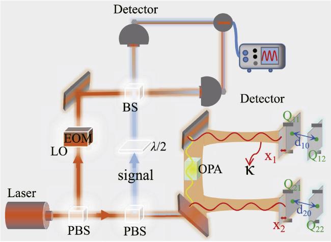
Figure 1. Schematic of the optomechanical system with homodyne detection. The local oscillator (LO) is phase-modulated with an electro-optical modulator (EOM). The two charged MOs interact with the two charged bodies through the Coulomb force respectively, and a degenerate optical parametric amplifier couples to a Fabry-Pérot cavity. |
The Hamiltonian of system can read as H = H0 + Hint + Hd (ℏ = 1).
$\begin{eqnarray}{H}_{0}={\omega }_{c}{a}^{\dagger }a+\displaystyle \sum _{j=1}^{2}{\omega }_{{jm}}{b}_{j}^{\dagger }{b}_{j}\end{eqnarray}$
describes the free energy of the system, where a and bj are the annihilation operators of the cavity field and the jth mechanical modes with resonant frequency ωc and ωjm, respectively; $\begin{eqnarray}\begin{array}{l}{H}_{\mathrm{int}}=\displaystyle \sum _{j=1}^{2}{g}_{{}_{j0}}{a}^{\dagger }a({b}_{j}+{b}_{j}^{\dagger })+F(t){x}_{{j}_{\mathrm{ZPF}}}({b}_{j}+{b}_{j}^{\dagger })\\ \,-\frac{{k}_{e}{C}_{j1}{U}_{j1}{C}_{j2}{U}_{j2}}{| {d}_{j0}+{x}_{j}| }\end{array}\end{eqnarray}$
denotes the various coupling of the optomechanical system. gj0 is the single photon optomechanical coupling strength with the jth MO, and ${x}_{{j}_{\mathrm{ZPF}}}=\sqrt{1/(2{m}_{j\mathrm{eff}}{\omega }_{{jm}})}$ is the zero-point fluctuation of the mechanical oscillator with the effective mass mjeff. The last two terms account for that the two mechanical modes interacts with the external measured force F and the two charged bodies respectively, where ke is the electrostatic constant, and Cj1Uj1 (−Cj2Uj2) is the positive (negative) charge on the charged MO (charged body) with Cj1 (Cj2) and Uj1 (−Uj2) being the capacitance and the voltage of the bias gate respectively. Considering displacement x1 of the first MO is smaller than the equilibrium distance d10 (The same method applies to the second MO), i.e. x1 ≪ d10, the Coulomb interaction can be truncate to second-order expansion $-\tfrac{{k}_{e}{C}_{11}{U}_{11}{C}_{12}{U}_{12}}{{d}_{10}}\left(1-\tfrac{{x}_{1}}{{d}_{10}}+\tfrac{{x}_{1}^{2}}{{d}_{10}^{2}}\right)$, where the linear term proportional to x1 can be absorbed into the redefinition of the equilibrium position of the MO [61, 67]. By omitting the constant terms, we can obtain the simplified Coulomb interaction as $-{k}_{e}{C}_{11}{U}_{11}{C}_{12}{U}_{12}{x}_{1}^{2}/{d}_{10}^{3}$ . The position and momentum operators can be read as ${x}_{j}={x}_{{j}_{\mathrm{ZPF}}}({{\rm{b}}}_{j}+{{\rm{b}}}_{j}^{\dagger })$ and ${p}_{j}={\rm{i}}{\left({m}_{j\mathrm{eff}}{\omega }_{{jm}}/2\right)}^{1/2}({{\rm{b}}}_{j}^{\dagger }-{b}_{j})$. So the Hamiltonian can be rewritten as $\begin{eqnarray}\begin{array}{rcl}{H}_{1} & = & {\omega }_{c}{a}^{\dagger }a+\displaystyle \sum _{j=1}^{2}({\omega }_{{jm}}-2{\xi }_{j}){b}_{j}^{\dagger }{b}_{j}\\ & & +\displaystyle \sum _{j=1}^{2}{g}_{{}_{j0}}{a}^{\dagger }a({b}_{j}+{b}_{j}^{\dagger })-{\xi }_{j}({b}_{j}^{2}+{b}_{j}^{\dagger 2})\\ & & +F(t){x}_{{j}_{\mathrm{ZPF}}}({b}_{j}+{b}_{j}^{\dagger })+{H}_{{\rm{d}}}\end{array}\end{eqnarray}$
with the effective mechanical coupling strength ${\xi }_{j}\,={k}_{e}{C}_{j1}{U}_{j1}{C}_{j2}{U}_{j2}/(2{m}_{j\mathrm{eff}}{\omega }_{{jm}}{d}_{j0}^{3})$. From the above equation, the ξj with selecting appropriate parameters can be a large value to enhance the nonlinearity. In order to diagonalize the mechanical nonlinearity, we introduce the Bogoliubov transformation, i.e. $B=\cosh (r)b-\sinh (r){b}^{\dagger }$ with the squeezing parameter $r=\mathrm{ln}[{\omega }_{m}/({\omega }_{m}-4\xi )]/4$ as [62]. The Hamiltonian can be read as $\begin{eqnarray}\begin{array}{ccl}{H}_{2} & = & {\omega }_{c}{a}^{\dagger }a+\displaystyle \sum _{j=1}^{2}{{\rm{\Omega }}}_{j}{B}_{j}^{\dagger }{B}_{j}\\ & & +\displaystyle \sum _{j=1}^{2}{g}_{{}_{j0}}{{\rm{e}}}^{{r}_{j}}{a}^{\dagger }a({{\rm{B}}}_{j}+{{\rm{B}}}_{j}^{\dagger })\\ & & +F(t){x}_{{j}_{\mathrm{ZPF}}}{{\rm{e}}}^{{r}_{j}}({{\rm{B}}}_{j}+{{\rm{B}}}_{j}^{\dagger })+{{\rm{H}}}_{{\rm{d}}},\end{array}\end{eqnarray}$
where the effective resonant frequency of MO ${{\rm{\Omega }}}_{j}={\omega }_{{jm}}{{\rm{e}}}^{-2{r}_{j}}$. By diagonalization, the mechanical nonlinearity produces a squeezing effect in the position direction, so that the couplings of both cavity field and external force to the MO have increased with the squeezing parameter rj, which is beneficial to amplify the SNR by adjusting the Coulomb coupling factors ξj compared to the absence of mechanical nonlinearity. $\begin{eqnarray}\begin{array}{l}{H}_{{\rm{d}}}=({\epsilon }_{{}_{1+}}^{* }{{\rm{e}}}^{{\mathrm{i\Omega }}_{1}t}+{\epsilon }_{{}_{1-}}^{* }{{\rm{e}}}^{-{\mathrm{i\Omega }}_{1}t}+{\epsilon }_{{}_{2+}}^{* }{{\rm{e}}}^{{\mathrm{i\Omega }}_{2}t}+{\epsilon }_{{}_{2-}}^{* }{{\rm{e}}}^{-{\mathrm{i\Omega }}_{2}t}){{\rm{e}}}^{{\rm{i}}{\omega }_{d}t}a\\ \,+h.c.+i{\rm{\Lambda }}({{\rm{e}}}^{-2{\rm{i}}{\omega }_{p}t}{a}^{\dagger 2}{{\rm{e}}}^{{\rm{i}}\theta }-{{\rm{e}}}^{2{\rm{i}}{\omega }_{p}t}{a}^{2}{{\rm{e}}}^{-{\rm{i}}\theta })\end{array}\end{eqnarray}$
represents the four cavity driving tones by the classical field with different amplitude and frequency [59, 68–71] as well as an OPA-assisted intracavity squeezing. These driving tones are applied with a squeezing of ${{\rm{e}}}^{-2{r}_{j}}$ $({{\rm{\Omega }}}_{j}={\omega }_{{jm}}{{\rm{e}}}^{-2{r}_{j}})$ from the mechanical sidebands, at ${\omega }_{d}\pm {\omega }_{1m}{{\rm{e}}}^{-2{r}_{1}}$ and ${\omega }_{d}\pm {\omega }_{2m}{{\rm{e}}}^{-2{r}_{2}}$, and are realized via the coupling capacitance between the cavities and a transmission line in a superconducting microcircuit [71].Now transform to an interaction picture with respect to ${H}_{0}^{1}={\omega }_{d}{a}^{\dagger }a+{\sum }_{j=1}^{2}{{\rm{\Omega }}}_{j}{B}_{j}^{\dagger }{B}_{j}$, and set ωp = ωd. The Hamiltonian can be rewritten as6 ), the optomechanical coupling writes sidebands onto the cavity output spectrum by the four-tone optical driving. The Heisenberg–Langevin equations are given as7 )–(8 ), considering in the resolved sideband regime, i.e. ωj ≫ κ, we can adopt the ansatz $a={a}_{{}_{0}}+{\alpha }_{{}_{1-}}{{\rm{e}}}^{{\rm{i}}{{\rm{\Omega }}}_{1}t}+{\alpha }_{{}_{1+}}{{\rm{e}}}^{-{\rm{i}}{{\rm{\Omega }}}_{1}t}+{\alpha }_{{}_{2-}}{{\rm{e}}}^{{\rm{i}}{{\rm{\Omega }}}_{2}t}\,+{\alpha }_{{}_{2+}}{{\rm{e}}}^{-{\rm{i}}{{\rm{\Omega }}}_{2}t}$, which clearly separates the Fourier components of the field at the driven sidebands [27]. For simplicity, we replace ${a}_{{}_{0}}$ with a, and equate frequency components. And the system dynamics can be obtained12 )–(15 ) with16 ), which can also take as a real number by an appropriate redefinition of phases. Defining ${X}_{j}=({B}_{j}+{B}_{j}^{\dagger })/\sqrt{2}$ and ${P}_{j}=-{\rm{i}}({B}_{j}-{B}_{j}^{\dagger })/\sqrt{2}$ (j = 1, 2), as well as $X=(a+{a}^{\dagger })/\sqrt{2}$ and $P={\rm{i}}({a}^{\dagger }-a)/\sqrt{2}$, represents the quadrature operators of the mechanical modes and cavity mode. Then the total effective Hamiltonian can be read as18 ), that is to say, the mechanical momentum Pj can also be seen as the observable value where the condition of the QND needs to satisfy [H∣F=0, Pj] = 0. From equation (18 ), it satisfies the XXi coupling form of typical QND so as to eliminate the backaction noise. Therefore, the four-tone driving with frequency resonance results in the XXi interaction with time independent. Besides, the OPA results in the direct coupling between momentum and position of cavity mode, which will modify the optical mode susceptibility.
$\begin{eqnarray}\begin{array}{c}{H}_{3}={\rm{\Delta }}{a}^{\dagger }a+\displaystyle \sum _{j=1}^{2}{g}_{{}_{j0}}{{\rm{e}}}^{{r}_{j}}{a}^{\dagger }a({B}_{j}{{\rm{e}}}^{-{\rm{i}}{{\rm{\Omega }}}_{j}t}+{B}_{j}^{\dagger }{{\rm{e}}}^{{\rm{i}}{{\rm{\Omega }}}_{j}t})\\ \quad +F(t){x}_{{j}_{\mathrm{ZPF}}}{{\rm{e}}}^{{r}_{j}}({{\rm{B}}}_{j}{{\rm{e}}}^{-{\rm{i}}{{\rm{\Omega }}}_{j}t}+{{\rm{B}}}_{j}^{\dagger }{{\rm{e}}}^{{\rm{i}}{{\rm{\Omega }}}_{j}t})\\ \quad +({\epsilon }_{{}_{1+}}^{* }{{\rm{e}}}^{{\rm{i}}{{\rm{\Omega }}}_{1}t}+{\epsilon }_{{}_{1-}}^{* }{{\rm{e}}}^{-{\rm{i}}{{\rm{\Omega }}}_{1}t}+{\epsilon }_{{}_{2+}}^{* }{{\rm{e}}}^{{\rm{i}}{{\rm{\Omega }}}_{2}t}+{\epsilon }_{{}_{2-}}^{* }{{\rm{e}}}^{-{\rm{i}}{{\rm{\Omega }}}_{2}t})a\\ \quad +h.c.+{\rm{i}}{\rm{\Lambda }}({a}^{\dagger 2}{{\rm{e}}}^{{\rm{i}}\theta }-{a}^{2}{{\rm{e}}}^{-{\rm{i}}\theta }),\end{array}\end{eqnarray}$
with cavity detuning Δ = ωc − ωd. From equation ( $\begin{eqnarray}\begin{array}{l}\dot{a}=-{\rm{i}}{\rm{\Delta }}a-{\rm{i}}\displaystyle \sum _{j=1}^{2}{g}_{{}_{j0}}{{\rm{e}}}^{{r}_{j}}a({B}_{j}{{\rm{e}}}^{-{\rm{i}}{{\rm{\Omega }}}_{j}t}+{B}_{j}^{\dagger }{{\rm{e}}}^{{\rm{i}}{{\rm{\Omega }}}_{j}t})\\ \quad -{\rm{i}}({\epsilon }_{{}_{1+}}{{\rm{e}}}^{-{\rm{i}}{{\rm{\Omega }}}_{1}t}+{\epsilon }_{{}_{1-}}{{\rm{e}}}^{{\rm{i}}{{\rm{\Omega }}}_{1}t}+{\epsilon }_{{}_{2+}}{{\rm{e}}}^{-{\rm{i}}{{\rm{\Omega }}}_{2}t}+{\epsilon }_{{}_{2-}}{{\rm{e}}}^{{\rm{i}}{{\rm{\Omega }}}_{2}t})\\ \quad +2{\rm{\Lambda }}{a}^{\dagger }{{\rm{e}}}^{{\rm{i}}\theta }-\displaystyle \frac{\kappa }{2}a+\sqrt{\kappa }{a}_{\mathrm{in}},\end{array}\end{eqnarray}$
$\begin{eqnarray}\begin{array}{c}\dot{{B}_{j}}=-{\rm{i}}{g}_{{}_{j0}}{{\rm{e}}}^{{r}_{j}}{{\rm{e}}}^{{\rm{i}}{{\rm{\Omega }}}_{j}t}{a}^{\dagger }a-\frac{{\gamma }_{j}}{2}{B}_{j}\\ \quad +\sqrt{{\gamma }_{j}}{B}_{j,\mathrm{in}}-{\rm{i}}{{Fx}}_{{j}_{\mathrm{ZPF}}}{{\rm{e}}}^{{r}_{j}}{{\rm{e}}}^{{\rm{i}}{{\rm{\Omega }}}_{j}t},\end{array}\end{eqnarray}$
where κ and γj are the decay of the cavity and mechanical modes, respectively. The input vacuum noise operator is shown by ain, satisfying the Markovian correlation functions $\langle {a}_{\mathrm{in}}(t){a}_{\mathrm{in}}^{\dagger }({t}^{{\prime} })\rangle =\delta (t-{t}^{{\prime} })$. Besides, for the MOs, the input Brownian noise can be rewritten with the Bogoliubov mode ${B}_{j,\mathrm{in}}=\cosh ({r}_{j}){b}_{j,\mathrm{in}}$-$\sinh ({r}_{j}){b}_{j,\mathrm{in}}^{\dagger }$ [72], which can be derived from the linear superposition of the Langevin equation for the original Hamiltonian. Thus the general correlation functions for two squeezed mechanical modes can be read as $\langle {B}_{j,\mathrm{in}}(t){B}_{j,\mathrm{in}}^{\dagger }({t}^{{\prime} })\rangle =({\bar{n}}_{j,\mathrm{th}}^{{\prime} }+1)\delta (t-{t}^{{\prime} })$, $\langle {B}_{j,\mathrm{in}}(t){B}_{j,\mathrm{in}}({t}^{{\prime} })\rangle \,=-\sinh (2{r}_{j})\left({\bar{n}}_{j,\mathrm{th}}+\tfrac{1}{2}\right)\delta (t-{t}^{{\prime} }),$ where ${\bar{n}}_{j,\mathrm{th}}^{{\prime} }=\cosh (2{r}_{j}){\bar{n}}_{j,\mathrm{th}}\,+{\sinh }^{2}({r}_{j})$, and ${\bar{n}}_{j,\mathrm{th}}={\left[\exp ({\omega }_{{jm}}/{\kappa }_{{\rm{B}}}{{\rm{T}}}_{{\rm{j}}})-1\right]}^{-1}$ is the mean number of thermal excitations of the jth MO at temperature Tj. Furthermore, the corresponding quadrature operator correlation functions are $\langle {X}_{j,\mathrm{in}}(t){X}_{j,\mathrm{in}}({t}^{{\prime} })\rangle =({\bar{n}}_{j,\mathrm{th}}+1/2){{\rm{e}}}^{-2{r}_{j}}\delta (t-{t}^{{\prime} })$ and $\langle {P}_{j,\mathrm{in}}(t){P}_{j,\mathrm{in}}({t}^{{\prime} })\rangle =({\bar{n}}_{j,\mathrm{th}}+1/2){{\rm{e}}}^{2{r}_{j}}\delta (t-{t}^{{\prime} })$, which indicates the squeezing direction is along the oscillator displacement direction. To solve the equations ( $\begin{eqnarray}\begin{array}{l}\dot{a}=-{\rm{i}}{\rm{\Delta }}a-{\rm{i}}{g}_{{}_{10}}{{\rm{e}}}^{{r}_{1}}({\alpha }_{{}_{1-}}{B}_{1}+{\alpha }_{{}_{1+}}{B}_{1}^{\dagger })\\ \quad +2{\rm{\Lambda }}{a}^{\dagger }{{\rm{e}}}^{{\rm{i}}\theta }-{\rm{i}}{g}_{{}_{20}}{{\rm{e}}}^{{r}_{2}}({\alpha }_{{}_{2-}}{B}_{2}+{\alpha }_{{}_{2+}}{B}_{2}^{\dagger })\\ \quad -\displaystyle \frac{\kappa }{2}a+\sqrt{\kappa }{a}_{\mathrm{in}},\end{array}\end{eqnarray}$
$\begin{eqnarray}\begin{array}{c}\dot{{B}_{1}}=-{\rm{i}}{g}_{{}_{10}}{{\rm{e}}}^{{r}_{1}}({\alpha }_{{}_{1-}}^{* }a+{\alpha }_{{}_{1+}}{a}^{\dagger })-\frac{{\gamma }_{1}}{2}{B}_{1}\\ \quad +\sqrt{{\gamma }_{1}}{B}_{1,\mathrm{in}}-{\rm{i}}{{Fx}}_{{1}_{\mathrm{ZPF}}}{{\rm{e}}}^{{r}_{1}}{{\rm{e}}}^{{\rm{i}}{{\rm{\Omega }}}_{1}t},\end{array}\end{eqnarray}$
$\begin{eqnarray}\begin{array}{c}\dot{{B}_{2}}=-{\rm{i}}{g}_{{}_{20}}{{\rm{e}}}^{{r}_{2}}({\alpha }_{{}_{2-}}^{* }a+{\alpha }_{{}_{2+}}{a}^{\dagger })-\frac{{\gamma }_{2}}{2}{B}_{2}\\ \quad +\sqrt{{\gamma }_{2}}{B}_{2,\mathrm{in}}-{\rm{i}}{{Fx}}_{{2}_{\mathrm{ZPF}}}{{\rm{e}}}^{{r}_{2}}{{\rm{e}}}^{{\rm{i}}{{\rm{\Omega }}}_{2}t},\end{array}\end{eqnarray}$
$\begin{eqnarray}\begin{array}{l}{\dot{\alpha }}_{{}_{1-}}=-{\rm{i}}({\rm{\Delta }}+{{\rm{\Omega }}}_{1}){\alpha }_{{}_{1-}}-{\rm{i}}{g}_{{}_{10}}{{\rm{e}}}^{{r}_{1}}{{aB}}_{1}^{\dagger }\\ \,+2{\rm{\Lambda }}{\alpha }_{{}_{1+}}^{* }{{\rm{e}}}^{{\rm{i}}\theta }-\displaystyle \frac{\kappa }{2}{\alpha }_{{}_{1-}}-{\rm{i}}{\epsilon }_{{}_{1+}}+\sqrt{\kappa }{a}_{{}_{1-,{in}}},\end{array}\end{eqnarray}$
$\begin{eqnarray}\begin{array}{l}{\dot{\alpha }}_{{}_{1+}}=-{\rm{i}}({\rm{\Delta }}-{{\rm{\Omega }}}_{1}){\alpha }_{{}_{1+}}-{\rm{i}}{g}_{{}_{10}}{{\rm{e}}}^{{r}_{1}}{{aB}}_{1}+2{\rm{\Lambda }}{\alpha }_{{}_{1-}}^{* }{{\rm{e}}}^{{\rm{i}}\theta }\\ \,-\displaystyle \frac{\kappa }{2}{\alpha }_{{}_{1+}}-{\rm{i}}{\epsilon }_{{}_{1-}}+\sqrt{\kappa }{a}_{{}_{1+,{in}}},\end{array}\end{eqnarray}$
$\begin{eqnarray}\begin{array}{l}{\dot{\alpha }}_{{}_{2-}}=-{\rm{i}}({\rm{\Delta }}+{{\rm{\Omega }}}_{2}){\alpha }_{{}_{2-}}-{\rm{i}}{g}_{{}_{20}}{{\rm{e}}}^{{r}_{2}}{{aB}}_{2}^{\dagger }+2{\rm{\Lambda }}{\alpha }_{{}_{2+}}^{* }{{\rm{e}}}^{{\rm{i}}\theta }\\ \,-\displaystyle \frac{\kappa }{2}{\alpha }_{{}_{2-}}-{\rm{i}}{\epsilon }_{{}_{2+}}+\sqrt{\kappa }{a}_{{}_{2-,{in}}},\end{array}\end{eqnarray}$
$\begin{eqnarray}\begin{array}{l}{\dot{\alpha }}_{{}_{2+}}=-{\rm{i}}({\rm{\Delta }}-{{\rm{\Omega }}}_{1}){\alpha }_{{}_{2+}}-{\rm{i}}{g}_{{}_{20}}{{\rm{e}}}^{{r}_{2}}{{aB}}_{2}+2{\rm{\Lambda }}{\alpha }_{{}_{2-}}^{* }{{\rm{e}}}^{{\rm{i}}\theta }\\ \,-\displaystyle \frac{\kappa }{2}{\alpha }_{{}_{2+}}-{\rm{i}}{\epsilon }_{{}_{2-}}+\sqrt{\kappa }{a}_{{}_{2+,{in}}}.\end{array}\end{eqnarray}$
Assuming the effective optomechanical couplings are relatively small compared to the larger driving strengths εj, thus the steady-state amplitudes of the field at the driven sidebands can be solved from equations ( $\begin{eqnarray}\langle {\alpha }_{{}_{j\pm }}\rangle =\displaystyle \frac{8{\rm{i}}{\rm{\Lambda }}{\epsilon }_{{}_{j\mp }}^{* }{{\rm{e}}}^{{\rm{i}}\theta }-4({\rm{\Delta }}\pm {{\rm{\Omega }}}_{j}){\epsilon }_{{}_{j\pm }}-2{\rm{i}}\kappa {\epsilon }_{{}_{j\pm }}}{{\kappa }^{2}-16{{\rm{\Lambda }}}^{2}+4({{\rm{\Delta }}}^{2}-{{\rm{\Omega }}}_{j}^{2})\mp 4{\rm{i}}\kappa {{\rm{\Omega }}}_{j}}.\end{eqnarray}$
We can obtain different steady-state amplitudes of cavity sidebands with various driving tones. Then the Hamiltonian can be obtained as $\begin{eqnarray}\begin{array}{c}H={\rm{\Delta }}{a}^{\dagger }a+{\rm{i}}{\rm{\Lambda }}({a}^{\dagger 2}{{\rm{e}}}^{{\rm{i}}\theta }-{a}^{2}{{\rm{e}}}^{-{\rm{i}}\theta })\\ \,+\displaystyle \sum _{j=1}^{2}{g}_{{}_{j0}}{{\rm{e}}}^{{r}_{j}}({\alpha }_{{}_{j-}}{a}^{\dagger }{B}_{j}+{\alpha }_{{}_{j+}}{a}^{\dagger }{B}_{j}^{\dagger }+{\rm{h}}.{\rm{c}}.)\\ \,+F(t){x}_{{j}_{\mathrm{ZPF}}}{{\rm{e}}}^{{r}_{j}}({B}_{j}{{\rm{e}}}^{-{\rm{i}}{{\rm{\Omega }}}_{j}t}+{B}_{j}^{\dagger }{{\rm{e}}}^{{\rm{i}}{{\rm{\Omega }}}_{j}t}).\end{array}\end{eqnarray}$
Furthermore, the cavity sideband amplitudes can be set ${\alpha }_{{}_{j\pm }}={\alpha }_{j}$ by the equation ( $\begin{eqnarray}\begin{array}{c}H=\left(\frac{{\rm{\Delta }}}{2}-{\rm{\Lambda }}\sin \theta \right){X}^{2}+(\frac{{\rm{\Delta }}}{2}+{\rm{\Lambda }}\sin \theta ){P}^{2}\\ \quad +X({G}_{1}{X}_{1}+{G}_{2}{X}_{2})+2{\rm{\Lambda }}{PX}\cos \theta \\ \quad +\displaystyle \sum _{j=1}^{2}\sqrt{2}F(t){x}_{{j}_{\mathrm{ZPF}}}({X}_{j}{{\rm{e}}}^{{r}_{j}}\cos {{\rm{\Omega }}}_{j}t+{P}_{j}{{\rm{e}}}^{{r}_{j}}\sin {{\rm{\Omega }}}_{j}t),\end{array}\end{eqnarray}$
where ${G}_{j}=2{g}_{{}_{j0}}{{\rm{e}}}^{{r}_{j}}{\alpha }_{{}_{j}}$ is the effective optomechanical coupling. In this system, due to the force signal inducing displacement of the oscillator, the mechanical displacement Xj can be regarded as the observable value reflecting the signal, where it needs to be met [H∣F=0, Xj] = 0 if the QND measurement is required. Then owing to the transformation of the Hamiltonian, the weak force is coupled to both the displacement and momentum of the oscillator in equation (3. Dynamics of the system
We now employ the effective Hamiltonian equation (18 ) to deduce the dynamics of the system by the Langevin equations as19 )–(22 ), we can see that the dynamics of the quadratures Xj and Pj of MO would not be simultaneously reflected in the cavity output, which surpasses the SQL caused by the non-commuting relationship between position and momentum of MO. In other words, the dynamics between equations (19 )–(20 ) are decoupling. As for the system stability, the dynamics equation can be rewritten as $\dot{u}={Mu}+{u}_{{}_{{in}}}$ from equations (19 )–(22 ), where $u={\left({X}_{1},{P}_{1},{X}_{2},{P}_{2},X,P\right)}^{T}$ and ${u}_{{}_{{in}}}={\left(\sqrt{{\gamma }_{1}}{X}_{1}^{{}_{{\rm{in}}}},\sqrt{{\gamma }_{1}}{P}_{1}^{{}_{{\rm{in}}}},\sqrt{{\gamma }_{2}}{X}_{2}^{{}_{{\rm{in}}}},\sqrt{{\gamma }_{2}}{P}_{2}^{{}_{{\rm{in}}}},\sqrt{\kappa }{X}_{{}_{{\rm{in}}}},\sqrt{\kappa }{P}_{{}_{{\rm{in}}}}\right)}^{T}$. The eigenvalues of the system can be written as Ev = ( − γ1/2 , −γ1/2 , −γ2/2 , −γ2/2, $-\kappa /2-\sqrt{4{{\rm{\Lambda }}}^{2}-{{\rm{\Delta }}}^{2}}$ , $-\kappa /2\,+\sqrt{4{{\rm{\Lambda }}}^{2}-{{\rm{\Delta }}}^{2}})$.Usually, the eigenvalues depend on the coupling Gj and OPA phase θ. Since the mechanical momentum Pj and coordinate Xj are dynamically independent of each other, the coupling Gj will not enter the expression of the eigenvalues. Besides the phase θ will be integrated in Ev due to trigonometric function relationship. Based on the Routh-Hurwitz criterion [73], all real parts of eigenvalues should be negative, where it just meets the requirements $\sqrt{4{{\rm{\Lambda }}}^{2}-{{\rm{\Delta }}}^{2}}-\kappa /2\lt 0$. To show the stable relationship of cavity detuning and OPA parameter more clearly, we plot figure 2, where the green area means the stable parameters for the system.
$\begin{eqnarray}\dot{{X}_{j}}=-\displaystyle \frac{{\gamma }_{j}}{2}{X}_{j}+\sqrt{{\gamma }_{j}}{X}_{j}^{\mathrm{in}},\end{eqnarray}$
$\begin{eqnarray}\dot{{P}_{j}}=-{G}_{j}X-\displaystyle \frac{{\gamma }_{j}}{2}{P}_{j}+\sqrt{{\gamma }_{j}}{P}_{j}^{\mathrm{in}},\end{eqnarray}$
$\begin{eqnarray}\dot{X}=({\rm{\Delta }}+2{\rm{\Lambda }}\sin \theta )P+2{\rm{\Lambda }}X\cos \theta -\displaystyle \frac{\kappa }{2}X+\sqrt{\kappa }{X}_{\mathrm{in}},\end{eqnarray}$
$\begin{eqnarray}\begin{array}{l}\dot{P}=-({\rm{\Delta }}-2{\rm{\Lambda }}\sin \theta )X-{G}_{1}{X}_{1}-{G}_{2}{X}_{2}-2{\rm{\Lambda }}P\cos \theta \\ \qquad -\displaystyle \frac{\kappa }{2}P+\sqrt{\kappa }{P}_{\mathrm{in}},\end{array}\end{eqnarray}$
where γj (j = 1, 2) and κ are the damping rate of the mechanical mode and cavity mode, respectively. In addition, the modified mechanical noise can be written as $\begin{eqnarray}{X}_{j}^{\mathrm{in}}(t)={X}_{j,\mathrm{in}}(t)+\sqrt{\displaystyle \frac{2}{\gamma }}{x}_{{j}_{\mathrm{ZPF}}}F(t){{\rm{e}}}^{{r}_{j}}\sin {{\rm{\Omega }}}_{j}t,\end{eqnarray}$
$\begin{eqnarray}{P}_{j}^{\mathrm{in}}(t)={P}_{j,\mathrm{in}}(t)-\sqrt{\displaystyle \frac{2}{\gamma }}{x}_{{j}_{\mathrm{ZPF}}}F(t){{\rm{e}}}^{{r}_{j}}\cos {{\rm{\Omega }}}_{j}t.\end{eqnarray}$
From equations (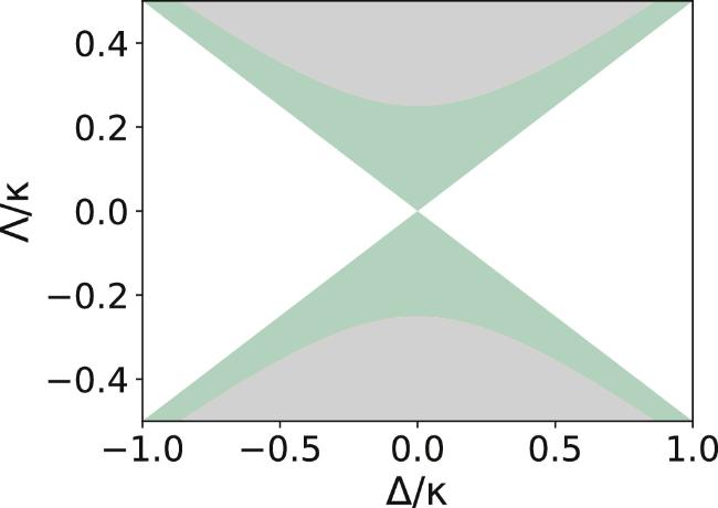
Figure 2. The stability of the system as a function of the cavity detuning Δ and the OPA parameter Λ, and the green area represents the stable parameters for the system according to $\sqrt{4{{\rm{\Lambda }}}^{2}-{{\rm{\Delta }}}^{2}}-\kappa /2\lt 0$. Other parameters are κ/γ = 106, and γ = 1. |
Equations (19 )–(22 ) can be solved in the frequency domain by performing the Fourier transformation. Within the standard input-output relation, ${O}_{\mathrm{out}}=\sqrt{\kappa }O-{O}_{\mathrm{in}}$, the output fields are related to the quadratures of the intracavity field with Xout(ω) and Pout(ω). We consider a homodyne measurement [29, 53, 54, 74] to sense the weak signal,25 ) denotes the total output includes the external signal, where the first curly bracket represents the thermal noise of two MOs and shot noise of the optical field, and the second square bracket mainly describes the additional effects as a result of the homodyne phase with φ ≠ nπ(n = 0, ±1, ±2, …).
$\begin{eqnarray}\begin{array}{l}T(\omega )=\sin \phi {X}_{\mathrm{out}}+\cos \phi {P}_{{}_{{out}}}\\ \quad =\sqrt{\kappa }{\chi }_{c}^{{\prime} }{u}_{\phi }\left\{\Space{0ex}{3.85ex}{0ex}-{G}_{1}{\chi }_{m1}\sqrt{{\gamma }_{1}}{X}_{1}^{\mathrm{in}}-{G}_{2}{\chi }_{m2}\sqrt{{\gamma }_{2}}{X}_{2}^{\mathrm{in}}\right.\\ \quad \left.+\sqrt{\kappa }\left[\left(1-\displaystyle \frac{1}{\kappa {\chi }_{c}^{{\prime} }}\right){P}_{\mathrm{in}}-{\chi }_{c}({\rm{\Delta }}-2{\rm{\Lambda }}\sin \theta ){X}_{\mathrm{in}}\right]\right\}\\ \quad +\sin \phi \left[(\kappa {\chi }_{c}-1){X}_{\mathrm{in}}+{\chi }_{c}({\rm{\Delta }}+2{\rm{\Lambda }}\sin \theta ){P}_{{}_{{in}}}\right],\end{array}\end{eqnarray}$
where φ accounts for the phase angle of the local oscillator and ${u}_{\phi }=\cos \phi +({\rm{\Delta }}+2{\rm{\Lambda }}\sin \theta ){\chi }_{c}\sin \phi $ has been defined. Equation (We note that the local oscillator phase can directly affect the phase quadrature of the optical output field, which changes the SNR [29, 75], though the local oscillator amplitude can increase the overall homodyne signal including noise and signal, which does not affect the SNR. So we focus on the impact of φ on the force sensing. A complete quantum state tomography can be achieved by adjusting the φ [76], moreover, it has been demonstrated that off-resonant force and displacement sensitivity reaching 1.5 dB below the SQL with strong quantum correlations in an optomechanical system by homodyne detection [77]. Besides, the susceptibilities of the cavity χc and MO χmj respectively are read
$\begin{eqnarray}\begin{array}{rcl}{\chi }_{c}(\omega ) & = & \displaystyle \frac{1}{\kappa /2-2{\rm{\Lambda }}\cos \theta -{\rm{i}}\omega },\\ {\chi }_{{mj}}(\omega ) & = & \displaystyle \frac{1}{{\gamma }_{j}/2-{\rm{i}}\omega }.\end{array}\end{eqnarray}$
We can see that the OPA indeed changes the cavity susceptibility when $\cos \theta \ne 0$. The modified mechanical noise and cavity mode susceptibility in frequency domain are $\begin{eqnarray}{X}_{j}^{\mathrm{in}}(\omega )={X}_{j,\mathrm{in}}-{\mathrm{ie}}^{{r}_{j}}{\overline{F}}_{-j},\end{eqnarray}$
$\begin{eqnarray}{\chi }_{c}^{{\prime} }(\omega )=\displaystyle \frac{1}{{\chi }_{c}(\omega )\left[{\left(\tfrac{\kappa }{2}-{\rm{i}}\omega \right)}^{2}+{{\rm{\Delta }}}^{2}-4{{\rm{\Lambda }}}^{2}\right]},\end{eqnarray}$
and the transduction force can be defined as ${\overline{F}}_{\pm j}\,=\sqrt{\tfrac{2}{\gamma }}\tfrac{{x}_{j\mathrm{ZPF}}}{2}[F(\omega +{{\rm{\Omega }}}_{j})\pm F(\omega -{{\rm{\Omega }}}_{j})]$.For equation (27 ), we need to require the same effective resonant frequency of two MOs, i.e. ω1 = ω2 = ω, so that the transduction force can be superimposed by coupling two MOs in the frequency domain. Furthermore, we can see that the signal has been enhanced owing to the nonlinear coupling between the charged body and MO.
4. Force sensing
For general cases of different dissipations, couplings and squeezed factors of the two oscillators, the noise of MO always can be rewritten in the form of ${ \mathcal X }{X}_{1,\mathrm{in}}\,+{ \mathcal Y }{X}_{2,\mathrm{in}}+({ \mathcal X }+{ \mathcal Y }){\overline{F}}_{-}$ in equation (25 ). For simplicity of calculation, we assume that the two oscillators have some of the same properties, i.e. squeezed parameters r1 = r2 = r, effective coupling G1 = G2 = G, and decay γ1 = γ2 = γ. As for equation (25 ), the first two terms in the curly bracket can be rewritten as $-G{\chi }_{m}\sqrt{\gamma }({X}_{1,\mathrm{in}}+{X}_{2,\mathrm{in}}-2{\mathrm{ie}}^{r}{\overline{F}}_{-})$, to calculate the sensitivity to the external force, so the generalized external force can be defined as [30, 53]:30 ), all noise, including thermal noise and shot noise, is suppressed by the squeezed factor. Similar to equation (25 ), the physical significance of each part does not change. In addition, the term proportional to the coupling is gone, in other words, the backaction noise has been evaded.
$\begin{eqnarray}{F}_{\mathrm{sum}}(\omega )=\frac{T(\omega )}{\partial T(\omega )/\partial {\bar{F}}_{-}}\equiv {F}_{{}_{\mathrm{add}}}(\omega )+{\bar{F}}_{-},\end{eqnarray}$
where the system can be regarded as the superposition of signal force and added noise force. ${F}_{{}_{\mathrm{add}}}(\omega )$ is given by $\begin{eqnarray}\begin{array}{c}{F}_{{}_{\mathrm{add}}}(\omega )=-\frac{{X}_{1,\mathrm{in}}+{X}_{2,\mathrm{in}}}{2{\mathrm{ie}}^{r}}\\ \quad +\sqrt{\frac{\kappa }{\gamma }}\frac{1}{2{\mathrm{ie}}^{r}G{\chi }_{m}}\left\{\left(1-\frac{1}{\kappa {\chi }_{c}^{^{\prime} }}\right){P}_{\mathrm{in}}\right.\\ \quad -{\chi }_{c}({\rm{\Delta }}-2{\rm{\Lambda }}\sin \theta ){X}_{\mathrm{in}}+\frac{{\rm{\Phi }}}{\kappa {\chi }_{c}^{^{\prime} }}\\ \quad \left.\times \left[(\kappa {\chi }_{c}-1){X}_{\mathrm{in}}+{\chi }_{c}({\rm{\Delta }}+2{\rm{\Lambda }}\sin \theta ){P}_{{}_{{in}}}\right]\right\}.\end{array}\end{eqnarray}$
Here we have defined ${\rm{\Phi }}=\sin \phi /{u}_{\phi }$. According to equation (To quantify the sensitivity of the force sensing, in general, the added noise force spectrum can be defined as [30, 78, 79]30 ) are respectively33 ), the first equation means the decreased thermal noise by the squeezed parameter e−4r. Furthermore, due to the dual-probe port, i.e. two oscillators coupling external force, the superposition effect on the signal is reflected in 1/4. If the system contains only one mechanical mode, the effective thermal noise of MO will be $({\bar{n}}_{{}_{1,\mathrm{th}}}+1/2){{\rm{e}}}^{-4r}$. Similar to the form of the effective Hamiltonian in this article, if one system can interact with n squeezed oscillators, the total effective thermal noise can be read as (X1,in + X2,in + X3,in + ⋯ + Xn,in + n/2)/(nier) with a similar method like the first term of equation (30 ). Furthermore, due to the lack of correlation between different noise, the power spectrum of total effective thermal noise can be rewritten as $({\sum }_{j=1}^{n}{\bar{n}}_{{}_{j,\mathrm{th}}}+n/2){{\rm{e}}}^{-4r}/{n}^{2}$. Moreover, the nadd(ω) in equation (33 ) refers to the noise contribution of the cavity field, which can also be reduced by the squeezed parameter e−4r owing to ∣G∣ ∝ er. According to equation (34 ), A and ${{ \mathcal B }}_{\phi }$ represent the cavity momentum noise, where ${{ \mathcal B }}_{\phi }$ results from the homodyne phase due to Φ, and for optical coordinate noise C and Dφ which are similar to A and ${{ \mathcal B }}_{\phi }$. Besides, in equation (33 ), the added noise contains parts with and without φ. Now we focus on optimizing the phase φ, where the added noise in equation (33 ) can be rewritten as36 ) can be simplified as36 ) the homodyne phase can be optimized so that the added noise spectrum is minimized,
$\begin{eqnarray}{S}_{\mathrm{add}\ }(\omega )\delta (\omega -{\omega }^{{\prime} })=\displaystyle \frac{{S}_{F}(\omega )+{S}_{F}(-{\omega }^{{\prime} })}{2},\end{eqnarray}$
where ${S}_{F}(\omega )=\langle {F}_{{}_{\mathrm{add}}}(\omega ){F}_{{}_{\mathrm{add}}}^{\dagger }(\omega )\rangle $. According to the correlation of vacuum cavity field and squeezed mechanical modes, the noise spectrum becomes $\begin{eqnarray}{S}_{\mathrm{add}\ }(\omega )={S}_{{\bar{{\rm{n}}}}_{{\rm{th}}}}+{n}_{\mathrm{add}},\end{eqnarray}$
where the mechanical thermal noise and added noise corresponding to the first and second terms of equation ( $\begin{eqnarray}\begin{array}{rcl}{S}_{{\bar{{\rm{n}}}}_{{\rm{th}}}} & = & \displaystyle \frac{{\bar{n}}_{{}_{1,\mathrm{th}}}+{\bar{n}}_{{}_{2,\mathrm{th}}}+1}{4}{{\rm{e}}}^{-4r},\\ {n}_{\mathrm{add}}(\omega ) & = & \displaystyle \frac{1}{2}\displaystyle \frac{\kappa {{\rm{e}}}^{-2r}}{4| G{\chi }_{m}{| }^{2}\gamma }\left({\left|A+{{ \mathcal B }}_{\phi }\right|}^{2}+{\left|C+{D}_{\phi }\right|}^{2}\right),\end{array}\end{eqnarray}$
with $\begin{eqnarray}\begin{array}{rcl}A & = & 1-\displaystyle \frac{1}{\kappa {\chi }_{c}^{{\prime} }},\quad C=-{\chi }_{c}({\rm{\Delta }}-2{\rm{\Lambda }}\sin \theta ),\\ {{ \mathcal B }}_{\phi } & = & \displaystyle \frac{{\rm{\Phi }}}{\kappa {\chi }_{c}^{{\prime} }}{\chi }_{c}({\rm{\Delta }}+2{\rm{\Lambda }}\sin \theta ),\quad {D}_{\phi }=\displaystyle \frac{{\rm{\Phi }}}{\kappa {\chi }_{c}^{{\prime} }}(\kappa {\chi }_{c}-1).\end{array}\end{eqnarray}$
For equation ( $\begin{eqnarray}{n}_{\mathrm{add}}(\omega )=\displaystyle \frac{1}{2}\displaystyle \frac{\kappa {{\rm{e}}}^{-2r}}{4| G{\chi }_{m}{| }^{2}\gamma }(| A{| }^{2}+| C{| }^{2}+{M}_{\phi }(\omega )),\end{eqnarray}$
where the phase part Mφ(ω) is $\begin{eqnarray}\begin{array}{l}{M}_{\phi }(\omega )=| {{ \mathcal B }}_{\phi }{| }^{2}+{A}^{* }{{ \mathcal B }}_{\phi }+A{{ \mathcal B }}_{\phi }^{* }\\ \quad +| {D}_{\phi }{| }^{2}+{C}^{* }{D}_{\phi }+{{CD}}_{\phi }^{* }.\end{array}\end{eqnarray}$
Only when the phase part meets Mφ(ω) < 0, the homodyne detection can be meaningful for sensing. When we focus on resonance, i.e. ω = 0, the equation ( $\begin{eqnarray}\begin{array}{rcl}{M}_{\phi }(0) & = & {{\rm{\Phi }}}^{2}(| { \mathcal B }{| }^{2}+| D{| }^{2})+2{\rm{\Phi }}(A{ \mathcal B }+{CD})\\ & = & {{\rm{\Phi }}}^{2}N+{\rm{\Phi }}E,\end{array}\end{eqnarray}$
where ${ \mathcal B }={\chi }_{c}({\rm{\Delta }}+2{\rm{\Lambda }}\sin \theta )/(\kappa {\chi }_{c}^{{\prime} })$, $D=(\kappa {\chi }_{c}-1)/(\kappa {\chi }_{c}^{{\prime} })$, $N=| { \mathcal B }{| }^{2}+| D{| }^{2}$, and $E=2(A{ \mathcal B }+{CD})$. Similar to the reference [54], for equation ( $\begin{eqnarray}\tan {\phi }_{\mathrm{opt}}={\left.\displaystyle \frac{-E}{2N+E{\chi }_{c}({\rm{\Delta }}+2{\rm{\Lambda }}\sin \theta )}\right|}_{\omega =0}.\end{eqnarray}$
when the φopt has been chosen, the coherent part can be obtain ${M}_{\phi }{\left(0\right)}_{\min }=-{E}^{2}/(4N)$.4.1. In the absence of OPA (Λ = 0)
From equations (26 ) and (28 ), the OPA affects the cavity output by the susceptibilities. In the case without OPA, i.e. Λ = 0, we are concerned about the changes in added noise. Firstly, we plot the added noise for the cavity detuning in figure 3(a), in which the blue dash-dotted line corresponds to φ = 0, while the orange solid line is optimized φopt. As we can see, when Δ = 0, the added noise can be minimized whether φ is optimized or 0. Nevertheless, the homodyne detection phase φopt will exert an advantage with Δ ≠ 0.
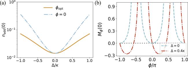
Figure 3. (a) The added noise nadd(0) versus cavity detuning. The blue dash-dotted line corresponds to φ = 0, while the orange solid line is optimized φopt. (b) The homodyne interference parts are taken as a function of the local oscillator phase φ/π, and the blue dashed line, as well as red dash-dotted responds to Δ/κ = 0, 0.4, respectively. Other parameters are taken as κ/γ = 106, γ = 1, r = 1, Λ = 0, and G/γ = 102 × er. |
Furthermore, figure 3(b) depicts the effect of local oscillator phase angle φ, where the blue dashed line and red dash-dotted respond to Δ/κ = 0, 0.4, respectively. The results reveal that the phase angle can not make an effective contribution on sensing when Δ = 0, but ${M}_{{\phi }_{\mathrm{opt}}}(0)$ can reduce added noise with Δ/κ = 0.4. From equation (18 ), the system Hamiltonian can be reduced to XX coupling, which is a typical QND type [36]. And as for the equation (21 ), the one of cavity quadrature X has been decoupled to the dynamics of the system owing to Δ = Λ = 0, so in equation (25 ) the part of phase with Xout becomes redundant for precision measurement. Besides, the analyzing results can be derived from equation (38 ). Due to Λ = Δ = 0, it can be derived with ${ \mathcal B }=C=E=0$, i.e. $\tan {\phi }_{\mathrm{opt}}=0$. When Δ ≠ 0, it can always find a suitable phase to satisfy ${M}_{\phi }{\left(0\right)}_{\min }\lt 0$, i.e. −E2/(4N) < 0.
4.2. With OPA assistance
In this section, we consider the case of the OPA in the cavity.
Firstly, we concentrate on optimizing the OPA parameter. In figures 4(a)–(b), we plot the added noise versus OPA strength Λ and phase θ when Δ = 0. From figure 4(a), the added noise almost does not vary with phase θ when Λ/κ ≈ 0.25 and Δ = 0, which can achieve the optimized results. In figure 4(b), the added noise is taken as a function of θ/π, where the cyan dashed line (purple dashed line), orange dash-dotted line (green dash-dotted line), and red solid line (gold solid line) curves, corresponds to Λ/κ = 0.24, 0.245, 0.249 and Δ = 0 with optimized homodyne phase φopt (φ = 0), respectively. We can see that all curves can reach the minimum values when θ = 0, which can be deduced from analytical expressions. Similar to the case without OPA, when Δ = θ = 0, it will result in ${ \mathcal B }=C=0$, and thus makes ${M}_{\phi }{\left(0\right)}_{\min }=0$, so the minima nadd(0) are coincident at θ = 0 which means the homodyne phase does not lead to better results. Nevertheless, without the assistance of homodyne interference, i.e. φ = 0, the OPA angle θ required to obtain the minimal added noise is more stringent. For the same parameters, like the red solid line and gold solid line curves with Λ/κ = 0.249, the optimization value taken with homodyne detection (φopt) has a broader requirement for phase angle θ than without homodyne detection (φ = 0). Furthermore, with the increase of Λ, the homodyne curves with φopt can obtain smaller values, but the curves value with φ = 0 becomes larger except for areas with θ ≈ 0, where it may not even break the SQL near θ = 0. In physics, as increasing Λ, the homodyne effect becomes prominent in reducing noise.
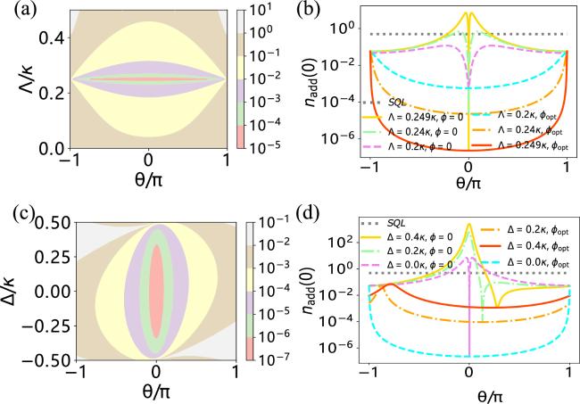
Figure 4. (a)–(b) The added noise nadd(0) is plotted as a function of the OPA phase θ and strength Λ when the resonance condition Δ = 0. (b) the gray dotted line corresponding the SQL, and the cyan dashed line, orange dash-dotted line, and red solid line curves corresponding to Λ/κ = 0.2, 0.24, 0.249. The upper lines represent the without homodyne interaction parts Mφ(0) = 0, the gold solid line, green dash-dotted line, and purple dashed line curves correspond to Λ/κ = 0.249, 0.24, 0.2. (c)–(d) The added noise versus θ and Δ when Λ/κ = 0.249. (d) the gray dotted line corresponds to the SQL, and the cyan dashed line, orange dash-dotted line, and red solid line curves correspond to Δ/κ = 0, 0.2, 0.4. The upper lines represent Mφ(0) = 0, the gold solid line, green dash-dotted line, and purple dashed line curves correspond to Δ/κ = 0.4, 0.2, 0. Other parameters are the same as those in figure 3. |
When we choose parameter Λ/κ = 0.249, we study how the cavity detuning Δ and OPA phase θ affect force sensing, as shown in figures 4(c)–(d). Similar to figures 4(a)–(b), when we consider the homodyne detection, in order to obtain less noise, there will be more tolerant for phase θ. The noise with homodyne detection, i.e. the cyan dashed line, orange dash-dotted line, and red solid line, increases with the switch of detuning Δ/κ = 0, 0.2, 0.4. So the less detuning, the less added noise. However, with the same parameters, including cyan and purple dashed lines, orange and green dash-dotted lines, as well as red and gold solid lines, the noise with optimal homodyne phase φopt can be achieved smaller values compared with the case of φ = 0 except the point of θopt. In particular, when we have optimized homodyne phase φopt, the OPA phase can be chosen from a broader range to obtain minimum noise, although it does not have an excessive impact on the reduction of added noise at θopt. Nevertheless, when the homodyne phase φ = 0 and cavity detuning Δ ≠ 0, not all the angles θ corresponding to the noise can break the SQL.
From the above analysis, with OPA assistance and without detuning, we need to enhance the strength Λ and decrease the phase angle θ. Concerning cavity detuning, smaller Δ can achieve smaller noise. Furthermore, though the system can obtain minimum added noise whether the local oscillator phase angle φ = 0 or optimized, it has relatively low parameter requirements for OPA phase θ fault tolerance with a homodyne optimized phase to decrease added noise, which reduces the difficulty of experiments.
4.3. Near-resonance ω ≈ 0
In this section, we consider the influence of system parameters on added noise in the case of near resonance (ω → 0). It is noted that the previously optimized homodyne phase φ is in the case of ω = 0 in equations (37 ) and (38 ). To investigate the error of optimizing the phase near resonance, we plot the homodyne phase φopt versus frequency ω/γ as shown in figure 5. The red line, orange line, and cyan line correspond to cavity detuning Δ = 0.4κ, 0.2κ, 0.1κ, and dashed lines represent φopt on resonance ω = 0 while dash-dotted lines mean the phase as a function of ω. At the near resonance, the dashed and dash-dotted lines can overlap. With the decreasing of cavity detuning, the ranges, where the angle difference Δφopt between corresponding dashed and dash-dotted lines is less than 1%φopt∣ω=0, becomes larger. Specially, when Δ = 0, the angel φopt does not change with ω due to φopt = 0. So we can conclude that the optimized homodyne phase φopt in equation (38 ) is still valid near resonance.
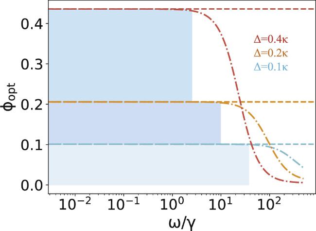
Figure 5. The homodyne optimized phase φ takes a function of frequency ω/γ. All dashed lines represent the optimized phase when ω = 0, while the dash-dotted lines denote the phase versus ω. The cyan line, orange line, and red line corresponds to Δ = 0.1κ, 0.2κ, 0.4κ, respectively. The colored areas indicate the angle φopt difference between the corresponding dashed and dash-dotted lines is less than 1%φopt∣ω=0. Other parameters are set as Λ/κ = 0.249 and θ = 0. |
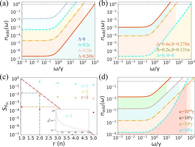
To investigate the impact of different parameters on noise in near resonance, we plot the variation of noise with different parameters in figure 6. For the sake of comparison, we plot the case of different OPA parameters Λ, and cavity detunings Δ with its corresponding optimized OPA phase θ which can be obtained in figure 4(d), as shown in figures 6(a)–(b). The result is confirmed in figures 4(b) and (d) on resonance, i.e. with the increasing of Λ and decreasing of Δ, the added noise can be greatly reduced. Besides, one can see that the range of signal frequency over which there is reducing noise, increase as we gradually optimize Λ and Δ in figures 6(a)–(b). Moreover, figure 6(c) shows the mechanical thermal noise is taken as a function of squeezed parameter r with red dash-dotted line and quantity of oscillator n with the colored dots. Obviously, as r and n increase, the thermal noise has been decreased, where the effect of noise reduction is more significant by increasing squeezed parameter r. Besides, the inset line represents the thermal noise versus the number of MOs when choosing r and other parameters. With the increase of oscillators, the noise can also be decreased, which provides a method for reducing effective thermal noise and enhancing the SNR. Furthermore, we study the contribution of cavity dissipation to added noise suppression in figure 6(d). The figure shows the noise reduction advantage is weakening as increasing the decay κ, but the noise can still reach the order of 10−3 with κ = 1010γ, which is also far greater than the SQL and beneficial for experimental implementation with the expansion of the parameters selection interval.
Figure 6. (a), (b) and (d) The added noise nadd(ω) takes a function of frequency ω/γ. The dotted blue line, cyan dashed line, orange dash-dotted line, and red solid line corresponds to the OPA parameter Λ = (0, 0.2κ, 0.24κ, 0.249κ) with Δ = θ = 0, respectively in (a). The red solid line, orange dash-dotted line, and cyan dashed line corresponds to the cavity detuning and optimized OPA phase (Δ, θ) = (0.4κ, 0.278π), (0.2κ, 0.131π), (0, 0) with Λ = 0.249κ, respectively in (b). The red solid line, brown dotted line, orange dash-dotted line, and cyan dashed line corresponds to the different cavity dissipations κ = 1010γ, 108γ, 106γ, 104γ with Δ = θ = 0, Λ = 0.249κ, respectively in (d). The dotted black lines denote the SQL. (c) The thermal noise ${S}_{{\bar{n}}_{\mathrm{th}}}$ as a function of squeezed parameter r with red dash-dotted line, and the quantity of oscillators n with cyan dots, orange dots, red dots correspond to r = 1, 2, 3 respectively. The inset line shows the noise versus the number of MOs when r = 1 and nth = 50. Other parameters are the same as those in figure 3. |
5. Signal-to-noise ratio and experiment discussion
In this section, we are concerned about the system sensitivity to the external force. In general, enhancing signal and reducing noise will be beneficial for precision measurement, and the SNR is a commonly quantified method for sensitivity. The SNR can be defined as [30, 34, 54, 80]32 ), viz., $\sqrt{{S}_{{}_{\mathrm{add}}}(\omega )}=\sqrt{{S}_{{\bar{{\rm{n}}}}_{{th}}}+{n}_{\mathrm{add}}}$. A well-detected system should achieve a suitable SNR, which means if r ≪ 1 then the signal will be submerged in noise, and if r ≫ 1 then it is a mismatch between the signal and detector. The minimum SNR which is the minimum detectable input of the device requires the minimum signal, i.e. r(ω) = 1 [81]. Therefore the sensitivity is $S(\omega )=\sqrt{{S}_{{}_{\mathrm{add}}}(\omega )}\sqrt{\gamma /2}/{x}_{{}_{\mathrm{ZPF}}}$. As shown in equation (39 ), the less added noise force, the more sensitive system detector. And the SNR can be increased by at least 2 orders of magnitude with the squeezed parameter and superimposed probe port when r = 1.
$\begin{eqnarray}r(\omega )=\frac{| {\bar{F}}_{-}(\omega )| }{\sqrt{{S}_{{}_{\mathrm{add}}}(\omega )}}.\end{eqnarray}$
As expected, the sensitivity of a force sensor depends on the added noise force spectrum consisting of mechanical thermal noise and cavity added noise in equation (Now we discuss the experimental implementation of this scheme. The Coulomb interaction between the charged MO and the charged body is experimentally feasible [61, 62, 82–85], which can be chosen the parameters as C1 = C2 = 27.5 nF , U1 = U2 = 1 V, d0 = 67 μm to achieve the effective mechanical coupling ξ ≈ GHz. Besides, the mechanical resonator frequency has already been demonstrated ω = GHz in micro- and nanofabricated optomechanical systems [86, 87], so that the charged body can match a relatively broad resonance frequency of MO. According to the squeezed parameter r definition, r can be obtained a large value due to 4ξ ≈ ωm, so that the signal can be greatly enhanced and noise is strongly depressed. Besides, the relationship between cavity decay and oscillator dissipation can also be implemented in a broader range of experimental systems to surpass the SQL from figure 6(d). Furthermore, the system can achieve ${\bar{n}}_{\mathrm{th}}=50$ at temperature T = 500 mK, when r = 1 and ${S}_{{\bar{n}}_{\mathrm{th}}}=2.3\times {10}^{-1}$, so the thermal phonon number of the oscillator is not required to be so low with cooling.
6. Conclusion
In this paper, we have introduced a four-tone setup aimed at force sensing in an optomechanical system, which has evaded backaction noise beyond the SQL. We show that when the driven tones are chosen correctly, the system can achieve an effective coupling XXj which is a QND typical form to avoid backaction noise. Besides, the coupling between the charged body and oscillator has provided nonlinear mechanical modes, which can increase force signal and decrease noise to promote sensitivity. The OPA can affect cavity susceptibility and thus benefit force detection.
Firstly, the stability of the system has been discussed based on the dynamics equation. Then for a more detailed discussion of force sensing, the case of resonance should be considered first. (i) In the absence of OPA, the added noise can obtain minimum value when cavity detuning Δ = 0 and homodyne phase angle φ = 0, and the homodyne detection does not work. When Δ ≠ 0, the φ can be optimized and the noise can be decreased compared with φ = 0. Whether the OPA parameter Λ and cavity detuning Δ is equal to zero or not, the system can still surpass the SQL, which is because the previous dynamics have avoided backaction noise by a QND method. (ii) When the OPA joins the cavity, the optimized OPA strength Λ and phase θ will further reduce the added noise by the cavity susceptibility. The Λ and θ can be optimized when Δ = 0, where the greater Λ, the better the effect of reducing noise. when Λ has been chosen, the smaller cavity detuning Δ, the lower the added noise, the optimized OPA phase θ will also change with Δ. Though the added noise can also reach minimum value without homodyne effect, the system can obtain a broader range parameter to achieve lower added noise with optimized homodyne detection. Next, the near-resonance is also considered. We find that the optimized homodyne phase φopt still works near-resonance. The different parameters, including OPA strength Λ, cavity detuning Δ, and optical dissipation κ, have been discussed in near-resonance. The result of near-resonance is consistent with that of on-resonance, where the larger Λ, and smaller Δ as well as κ, can not only reduce added noise but also increase the bandwidth of signal frequency. Furthermore, increasing the squeezed parameter r or the number of oscillators can decrease the mechanical thermal noise. Finally, the SNR indicates the better sensitivity of the system requires less noise including mechanical thermal and cavity added noise. Our work provides new insight in enhancing the SNR of a force sensor, which can be extended to other sensing, such as mass sensors, charge sensors, and quantum magnetometers.