


1. Introduction
The construction of gravitational modifications, namely extended gravity theories with general relativity (GR) as a specific constraint but with generally richer structures [1], is motivated by both theoretical and observational implications. The initial proposal depends on the concept that, due to the fact that GR does not seem renormalizable, we might presume that its more intricate extensions will have better renormalizability attributes [2]. The necessity to characterize the Universe's two accelerated phasesone in the early universe (inflation) and one in the late universe (the dark energy era) is the second motive. It is tied to the observable characteristics of the Universe. Starting with the Einstein–Hilbert action and extending it in different ways [3] is the typical method for constructing gravitational modifications. However, starting with the teleparallel equivalent of general relativity (TEGR) [4–6], which is the analogous torsional formulation for gravity, we can manipulate it to arrive at f(T) gravity [7–9], $f(T,{{ \mathcal T }}_{G})$ gravity [10], $f(T,{ \mathcal B })$ gravity [11, 12], scalar-torsion theories [13–15], etc.
An alternative geometrical theory of gravity known as TEGR was developed by Albert Einstein using absolute parallelism and the tangent space as a frame of reference [16]. At every point in tangent space, an orthogonal tetrad is generated in TEGR and can therefore be employed as a dynamical variable [17]. The torsion in space-time, which may be determined using a torsion tensor, defines the gravitational influence in TEGR. A torsion scalar is used to describe the effect of gravity, and the tetrad field is used as one of the theory's dynamical variables to generate the field equation for TEGR. The action of TEGR may now be modified for generating f(T) gravity by employing a more general function of torsion scalar [18]. The f(T) gravity has recently been shown to be incredibly effective in interpreting a variety of celestial observations [19–23]. It has been established that the galactic dynamics and cosmic expansions can both be explained quite well by the f(T) gravity theory. In [24], the effective field theory is put forward in a systematic approach to explain torsion gravity. Moreover, the gravitational wave propagation bound from GW170817 and GRB170817A are two examples of how this approach of effective field theory description and application of specific operators, including torsional terms, by observational constraints has already demonstrated its effectiveness in interpreting stellar phenomena. The combined interpretation of H0 and Σ8 tensions has recently also been investigated by Yan and colleagues [25].
Studying the physical attributes of compact stellar objects using teleparallel gravity is also useful for understanding their nature [26–30]. Teleparallel gravity and other modified gravities are employed for modeling compact stellar objects like strange stars, neutron stars, wormholes, and black holes [31–35]. Typically, compact stars are modeled using the isotropic stellar configuration. The stellar structures of the stars' interiors, however, contain anisotropic matter distributions, as evidenced by recent observations of compact stellar objects like 4U 1820–30, 4U 1538–52, and PSRJ 1614–2230. The anisotropic nature of stellar configurations [36, 37] is due to the uneven distribution of matter caused by phase transitions and the pion condensations in the type III-A superfluids identified within such stellar objects. The stellar rotation and electromagnetic field are thoroughly investigated to identify the anisotropy of the stars. Hence, in view of their physical significance, tremendous endeavors have been put into modeling compact stars, taking into account their intrinsic anisotropy [38–43].
Significant attempts are underway to describe compact stellar configurations using modified theories of gravity in order to shed light on some remarkable observations of them [44, 45]. Moreover, the study of anisotropic compact stellar structures with diagonal and off-diagonal tetrads in f(T) gravity has been extensively explored [46–48]. Besides that, an analysis of spherically symmetric stellar structures in f(T) gravity based on diagonal tetrad yields necessities on f(T) for being a linear function of T, thereby making the theory fundamentally TEGR [18].
On the other hand, the structure of a spherically symmetrical object in hydrostatic equilibrium may be modeled using generalized Tolman–Oppenheimer–Volkoff (TOV) [49] equations, which are derivations from the gravity theory. Equations are derived through the Einstein–Hilbert action of GR and may be employed, for instance, to characterize neutron stars. The maximum mass allowed for these sorts of stars for a specific equation of state can be calculated, among other things, via these generalized TOV equations. In this way, taking various gravity models into account may theoretically result in different maximum masses; for further information, see [50]. For instance, this could turn out to be crucial in explaining one of the elements of event GW190814 [51], which featured the coalescence of a black hole with a mass of 22.20–24.30 M⊙ and a compact object with a mass of 2.50–2.67 M⊙, the latter of which may have been an extremely high-mass neutron star or a low-mass black hole. Therefore, it is quite obvious that it is worth considering other gravitational models, such as f(T) models, when describing compact objects.
In this paper, we developed an analytical relativistic anisotropic quintessence spherical model within the framework of f(T) gravity theory, driven by all of the preceding arguments. Regarding this, we imposed some ingredients by considering the pressure anisotropy condition and the metric potential of the TK type, which serve as the main pillars of the resulting paradigm. Along with the anisotropic matter distribution, we also assume that our current model includes a quintessence field, defined by a parameter ωq, and then study the stability of motion and thermodynamic properties.
The manuscript is organized in the following way: in section 2 , we briefly describe the interior spacetime and Einstein equations in the f(T) theory. In section 3 , we address analytically relativistic quintessence anisotropic spherical solutions in the context of f(T) gravity. In both sections 4 and 5 , the matching of the internal and exterior Schwarzschild solutions at the boundary of stellar surfaces and the analysis of motion stability and thermodynamic characteristics are investigated. Using the M−R curve and the TOV equation, the predicted mass and radius of stars that may exist in nature are listed in section 6 . The overall summary and a few final concluding remarks on the investigation are addressed in section 7 .
2. Interior spacetime and Einstein equation in f(T) theory
When considering static geometry for stellar formations with spherically symmetric matter distribution, spacetime is described by the following line element,
$\begin{eqnarray}{\rm{d}}{s}^{2}={{\rm{e}}}^{\nu (r)}{{\rm{d}}{t}}^{2}-{{\rm{e}}}^{\lambda (r)}{{\rm{d}}{r}}^{2}-{r}^{2}({\rm{d}}{\theta }^{2}+{\sin }^{2}\theta {\rm{d}}{\phi }^{2}).\end{eqnarray}$
Here, the metric coefficients eν(r) and eλ(r) are pure radial functions of r.With the help of the matrix transformation known as the tetrad, the line element (1 ) can be transformed into a Minkowskian space as follows:
$\begin{eqnarray}{\rm{d}}{s}^{2}={g}_{\mu \nu }{\rm{d}}{x}^{\mu }{\rm{d}}{x}^{\nu }={\eta }_{\mathrm{ij}}{\theta }^{{\rm{i}}}{\theta }^{{\rm{j}}},\end{eqnarray}$
$\begin{eqnarray}{\rm{d}}{x}^{\mu }={{\rm{e}}}_{{\rm{i}}}^{\mu }{\theta }^{{\rm{i}}},\,{\theta }^{{\rm{i}}}={{\rm{e}}}_{\mu }^{{\rm{i}}}{\rm{d}}{x}^{\mu }.\end{eqnarray}$
where ηij = diag(1, −1, −1, −1) and ${{\rm{e}}}_{{\rm{i}}}^{\mu }{{\rm{e}}}_{\nu }^{{\rm{i}}}={\delta }_{\nu }^{\mu }$. The determinant of the metric g is connected to the determinant of the tetrad $e=\sqrt{-g}=\det ({{\rm{e}}}_{\mu }^{{\rm{i}}})$.We start with the action of the f(T) theory given as [9, 52]:
$\begin{eqnarray}S[{{\rm{e}}}_{\mu }^{{\rm{i}}},{\phi }_{A}]=\int {{\rm{d}}}^{4}x\,e\,\left[\displaystyle \frac{1}{16\pi }f(T)+{{ \mathcal L }}_{\mathrm{matter}}({\phi }_{A})\right].\end{eqnarray}$
Here, φA represents matter fields, and f(T) is an arbitrary analytic function of the torsion scalar T. Here the expression of the torsion scalar is given as follows: $\begin{eqnarray}T={S}_{\sigma }^{\,\,\mu \nu }{T}_{\mu \nu }^{\,\,\sigma },\end{eqnarray}$
where the tensor ${S}_{\sigma }^{\mu \nu }$ is described as [28], $\begin{eqnarray}{S}_{\sigma }^{\,\mu \nu }=\displaystyle \frac{1}{2}\left({K}_{\,\,\,\sigma }^{\mu \nu }+{\delta }_{\sigma }^{\mu }{T}_{\beta }^{\beta \nu }-{\delta }_{\sigma }^{\nu }{T}_{\,\,\,\beta }^{\beta \mu }\right).\end{eqnarray}$
and, $\begin{eqnarray}{T}_{\mu \nu }^{\sigma }={{\rm{\Gamma }}}_{\,\nu \mu }^{\sigma }-{{\rm{\Gamma }}}_{\,\mu \nu }^{\sigma }={{\rm{e}}}_{{\rm{i}}}^{\,\sigma }\left({\partial }_{\mu }{{\rm{e}}}_{\,\nu }^{{\rm{i}}}-{\partial }_{\nu }{{\rm{e}}}_{\,\mu }^{{\rm{i}}}\right),\end{eqnarray}$
$\begin{eqnarray}{K}_{\,\,\sigma }^{\mu \nu }=-\displaystyle \frac{1}{2}\left({T}_{\,\,\,\sigma }^{\mu \nu }-{T}_{\,\,\,\sigma }^{\nu \mu }-{T}_{\sigma }^{\,\mu \nu }\right).\end{eqnarray}$
By varying the action with respect to the tetrads, the field equations of f(T) gravity can be obtained as [52]
$\begin{eqnarray}\begin{array}{l}{S}_{\mu }^{\,\nu \rho }{\partial }_{\rho }{{Tf}}_{{TT}}+\left[{{\rm{e}}}^{-1}{{\rm{e}}}_{\mu }^{{\rm{i}}}{\partial }_{\rho }(e{{\rm{e}}}_{{\rm{i}}}^{\,\alpha }{S}_{\alpha }^{\,\nu \rho })\right]{f}_{T}\\ \quad +\displaystyle \frac{1}{4}{\delta }_{\mu }^{\nu }f=4\pi {T}_{\mu }^{\nu },\end{array}\end{eqnarray}$
where $\begin{eqnarray}{f}_{T}=\displaystyle \frac{\partial f}{\partial T}\,\,\,\,{f}_{{TT}}=\displaystyle \frac{{\partial }^{2}f}{\partial {T}^{2}}.\end{eqnarray}$
Here, ∂μ stands for partial derivative with respect to four coordinates xμ, (xμ stands for t, r, θ, φ), and $e=\det ({{\rm{e}}}_{\mu }^{{\rm{i}}})={{\rm{e}}}^{\tfrac{\lambda +\nu }{2}}{r}^{2}\sin \theta $, and the expression for the torsion scalar is given as, $\begin{eqnarray}T(r)=\displaystyle \frac{2{{\rm{e}}}^{-\lambda }}{r}\left(\nu ^{\prime} +\displaystyle \frac{1}{r}\right).\end{eqnarray}$
Here ${T}_{\mu }^{\nu }$ is the energy-momentum tensor of the underlying fluid. Let us assume that our model includes an anisotropic fluid that represents regular baryonic matter and a quintessence field.The energy-momentum tensor for normal baryonic matter is given by,
$\begin{eqnarray}{{ \mathcal T }}_{\mu }^{\nu }=\mathrm{diag}(\rho ,-{p}_{r},-{p}_{t},-{p}_{t}),\end{eqnarray}$
where ρ, pr, and pt, respectively, represent the energy density, radial pressure, and transverse pressure of normal matter.Furthermore, let us assume that ${\tau }_{\mu }^{\nu }$ represents the energy-momentum tensor for the quintessence field, and its non-zero components are given by,
$\begin{eqnarray*}\begin{array}{rcl}{\tau }_{r}^{r} & = & {\tau }_{t}^{t}=-{\rho }_{q},\\ {\tau }_{\theta }^{\theta } & = & {\tau }_{\phi }^{\phi }=\displaystyle \frac{(3\omega +1){\rho }_{q}}{2},\end{array}\end{eqnarray*}$
here ρq represents the energy density for the quintessence field characterized by the parameter ω, with ($-1\lt \omega \lt -\tfrac{1}{3}$), and $\begin{eqnarray}{T}_{\mu }^{\nu }={{ \mathcal T }}_{\mu }^{\nu }+{\tau }_{\mu }^{\nu }.\end{eqnarray}$
The field equations in f(T) gravity for the underlying fluid are given by, $\begin{eqnarray}\begin{array}{l}4\pi \left(\rho +{\rho }_{q}\right)=\displaystyle \frac{f}{4}-\left[T-\displaystyle \frac{1}{{r}^{2}}-\displaystyle \frac{{{\rm{e}}}^{-\lambda }}{r}(\lambda ^{\prime} +\nu ^{\prime} )\right]\displaystyle \frac{{f}_{T}}{2}\\ \,-\displaystyle \frac{{{\rm{e}}}^{-\lambda }}{r}T^{\prime} {f}_{{TT}},\end{array}\end{eqnarray}$
$\begin{eqnarray}4\pi \left({p}_{r}-{\rho }_{q}\right)=\left[T-\displaystyle \frac{1}{{r}^{2}}\right]\displaystyle \frac{{f}_{T}}{2}-\displaystyle \frac{f}{4},\end{eqnarray}$
$\begin{eqnarray}\begin{array}{l}4\pi \left({p}_{t}+\displaystyle \frac{3\omega +1}{2}{\rho }_{q}\right)=\left[\displaystyle \frac{T}{2}+{{\rm{e}}}^{-\lambda }\left\{\displaystyle \frac{\nu ^{\prime\prime} }{2}\right.\right.\\ \ +\left.\left.\left(\displaystyle \frac{\nu ^{\prime} }{4}+\displaystyle \frac{1}{2r}\right)(\nu ^{\prime} -\lambda ^{\prime} )\right\}\right]\displaystyle \frac{{f}_{T}}{2}-\displaystyle \frac{f}{4}+\displaystyle \frac{{{\rm{e}}}^{-\lambda }}{2}\left(\displaystyle \frac{\nu ^{\prime} }{2}+\displaystyle \frac{1}{r}\right)T^{\prime} {f}_{{TT}},\end{array}\end{eqnarray}$
$\begin{eqnarray}\mathrm{and}\,\,\,\,{{\rm{e}}}^{-\tfrac{\lambda }{2}}\displaystyle \frac{\cot \theta }{2{r}^{2}}T^{\prime} {f}_{{TT}}=0.\end{eqnarray}$
Here, ‘prime' denotes differentiation with respect to the radial coordinate ‘r'.For the choice of f(T) = T, the aforementioned field equations (14 )–(16 ) lead to the corresponding field equations in GR.
Now the equation (17 ) gives two choices: (i) $T^{\prime} =0$ or (ii) fTT = 0. In the second case, one obtains a linear form of the f(T) function as
$\begin{eqnarray}f(T)=\alpha T+\beta ,\end{eqnarray}$
where α and β are constants of integration.If we choose $T^{\prime} =0$ instead of fTT = 0, it gives a constant torsion scalar, T = T0. With the choice of T = T0, the right side of the equation (15 ) blows up as r → 0. This implies that the pressure of the substance is not finite; therefore, we exclude this case.
3. Our present model
With the choice of f(T) function given in equation (18 ), from the equations (14 )–(15 ), we arrived at the following equation:
$\begin{eqnarray}\rho +{p}_{r}=\displaystyle \frac{\alpha }{8\pi r}{{\rm{e}}}^{-\lambda }(\lambda ^{\prime} +\nu ^{\prime} ).\end{eqnarray}$
At this stage, let us assume that the metric potentials eν(r) and eλ(r) are of TK type, i.e.$\begin{eqnarray*}\nu (r)={{Br}}^{2}+2\mathrm{ln}D,\mathrm{and}\,\,\lambda (r)=\mathrm{ln}(1+{{ar}}^{2}+{{br}}^{4}),\end{eqnarray*}$
here, a, b, B, D, are all arbitrary constants, and their value can be obtained by a smooth matching of interior and exterior spacetime at the boundary.Using the TK metric potential, we will discuss some earlier research on the compact star model. Bhar [53] developed a new model of an anisotropic compact star with a TK metric potential using f(T) gravity. The author examined the thermodynamical characteristics of the model by using observational data from the compact star LMC X-4. A compact star associated with dark energy was hypothesized by Saklany et al [54] utilizing the TK metric potential. The author chose the super-dense pulsar PSRJ1614-2230 as the model star to discuss the physical analysis. In the context of the TK metric and modified f(R, G) gravity, Javed et al [55] described the behavior of anisotropic stellar spheres. Using metric potentials of the TK type, Biswas et al [56] explored an anisotropic, spherically symmetric strange star in a background of f(R, T) gravity. The suggested model satisfies stability criteria, is well-behaved, and is devoid of singularities.
Using the expressions of the metric coefficients, the equation (19 ) takes the following form:
$\begin{eqnarray}\rho +{p}_{r}=\displaystyle \frac{\alpha }{4\pi }\left[\displaystyle \frac{a+2{{br}}^{2}}{1+{{ar}}^{2}+{{br}}^{4}}+B\right].\end{eqnarray}$
Let us further suppose that the energy density ρ and the radial pressure pr maintain a linear relationship given as $\begin{eqnarray}{p}_{r}=\gamma \rho -\delta ,\end{eqnarray}$
where γ and δ are arbitrary positive constants with 0 < γ < 1.Now, using the above relationship, the field equations are solved, and the expressions of the parameters are obtained as follows,
$\begin{eqnarray}\rho =\displaystyle \frac{1}{4(1+\gamma )}\left[\displaystyle \frac{(a+B+(2b+{aB}){r}^{2}+{{bBr}}^{4})\alpha }{\pi {\left(1+{{ar}}^{2}+{{br}}^{4}\right)}^{2}}+4\delta \right],\end{eqnarray}$
$\begin{eqnarray}\begin{array}{l}{\rho }_{q}=\displaystyle \frac{1}{16\pi (1+\gamma )}\\ \times \ \left[(1+\gamma )\beta +2\left\{\displaystyle \frac{\alpha \left((a-2B+{{br}}^{2})(1+{{ar}}^{2}+{{br}}^{4})+\left(3a+({a}^{2}+b){r}^{2}+2{{abr}}^{4}+{b}^{2}{r}^{6}\right)\gamma \right)}{{\left(1+{{ar}}^{2}+{{br}}^{4}\right)}^{2}}-8\pi \delta \right\}\right],\end{array}\end{eqnarray}$
$\begin{eqnarray}\begin{array}{l}{p}_{r}=\displaystyle \frac{1}{4(1+\gamma )}\left[\displaystyle \frac{\left(a+B+(2b+{aB}){r}^{2}+{{bBr}}^{4}\right)\alpha \gamma }{\pi {\left(1+{{ar}}^{2}+{{br}}^{4}\right)}^{2}}-4\delta \right],\end{array}\end{eqnarray}$
$\begin{eqnarray}\begin{array}{l}{p}_{t}=\displaystyle \frac{1+3\omega }{32\pi {\left(1+{{ar}}^{2}+{{br}}^{4}\right)}^{2}}\left[-\beta {\left(1+{{ar}}^{2}{{br}}^{4}\right)}^{2}-2\left\{{a}^{2}{r}^{2}\alpha +2{{abr}}^{4}\alpha \right.\right.\\ +\ \displaystyle \frac{\alpha \left(a(1-2{{Br}}^{2}+3\gamma )-2B(1+{{br}}^{4})+{{br}}^{2}(1+5\gamma +{{br}}^{4}(1+\gamma ))\right)-8\pi {\left(1+{{ar}}^{2}+{{br}}^{4}\right)}^{2}\delta }{1+\gamma }\\ \left.\left.-\ \displaystyle \frac{2\left(2B-a+(-2b+B(a+B)){r}^{2}+{{aB}}^{2}{r}^{4}+{{bB}}^{2}{r}^{6}\right)\alpha -{\left(1+{{ar}}^{2}+{{br}}^{4}\right)}^{2}\beta }{1+3\omega }\right\}\right].\end{array}\end{eqnarray}$
For our current model, the central density and central pressure are obtained as follows,$\begin{eqnarray*}{\rho }_{c}=\rho (r=0)=\displaystyle \frac{a\alpha +B\alpha +4\pi \delta }{4(1+\gamma )},\end{eqnarray*}$
$\begin{eqnarray*}{p}_{r}(r=0)=\displaystyle \frac{(a+B)\alpha \gamma -4\pi \delta }{4(1+\gamma )},\end{eqnarray*}$
$\begin{eqnarray*}{p}_{t}(r=0)=\displaystyle \frac{4\alpha B(3+2\gamma +3\omega )-2a\alpha (3+5\gamma +3\omega +9\gamma \omega )+16\delta \pi -3(\beta (1+\gamma )(1+\omega )-16\delta \omega \pi )}{32(1+\gamma )\pi },\end{eqnarray*}$
and therefore the anisotropic factor Δ at the origin is obtained as,$\begin{eqnarray*}{\rm{\Delta }}(r=0)=-\displaystyle \frac{3(1+\omega )(-4\alpha B+\beta +\beta \gamma +2a(\alpha +3\alpha \gamma )-16\delta \pi )}{32(1+\gamma )\pi }.\end{eqnarray*}$
For a physically acceptable model, the anisotropic factor should vanish at the center of the star, which gives $\begin{eqnarray}-4\alpha B+\beta +\beta \gamma +2a(\alpha +3\alpha \gamma )-16\delta \pi =0.\end{eqnarray}$
In the next sections, we are going to check the boundary condition and the physical viability of our present model via different tests.Table 1. The numerical values of a, B and D for some well known compact objects by assuming b = 0.1 × 10⁻⁴ km−4. |
| Star | Observed mass | Observed radius | Estimated | Estimated | a | B | D |
|---|---|---|---|---|---|---|---|
| M⊙ | km. | mass (M⊙) | radius (km) | km−2 | km−2 | ||
| Her X-1 [67] | 0.85 ± 0.15 | 8.1 ± 0.41 | 0.85 | 8.5 | 0.005 430 30 | 0.002 895 78 | 0.756 246 |
| SMC X-4 [68] | 1.29 ± 0.05 | 8.831 ± 0.09 | 1.29 | 8.8 | 0.009 451 88 | 0.004 919 54 | 0.622 699 |
| 4U 1538–52 [68] | 0.87 ± 0.07 | 7.866 ± 0.21 | 0.87 | 7.8 | 0.007 756 26 | 0.004 030 23 | 0.724 610 |
| Vela X-1 [68] | 1.77 ± 0.08 | 9.56 ± 0.08 | 1.77 | 9.5 | 0.013 071 20 | 0.006 761 24 | 0.494 630 |
| Cen X-3 [68] | 1.49 ± 0.08 | 9.178 ± 0.13 | 1.49 | 9.2 | 0.010 385 80 | 0.005 404 49 | 0.574 909 |
| LMC X-4 [68] | 1.04 ± 0.09 | 8.301 ± 0.2 | 1.04 | 8.3 | 0.008 167 55 | 0.004 256 00 | 0.685 691 |
| EXO 1785–248 [69] | 1.3 ± 0.2 | 8.849 ± 0.4 | 1.4 | 8.85 | 0.010 780 10 | 0.005 585 88 | 0.586 810 |
Table 2. Central density, surface density, central pressure, compactness factor, and surface redshift have been presented for the compact star Her X-1 [67] for different values of α. |
| α | ρc | ρs | pc | u(R) | zs(R) |
|---|---|---|---|---|---|
| 0.5 | 3.9184 × 10¹⁴ | 2.834 28 × 1014 | 3.219 83 × 1034 | 0.011 5149 | 0.011 7177 |
| 1.08 | 7.836 79 × 1014 | 5.668 56 × 1014 | 6.439 66 × 1034 | 0.023 0299 | 0.023 8572 |
| 1.5 | 1.175 52 × 1015 | 8.502 83 × 1014 | 9.659 48 × 1034 | 0.034 5448 | 0.036 4445 |
| 2.0 | 1.567 36 × 1015 | 1.133 71 × 1015 | 1.287 93 × 1035 | 0.046 0597 | 0.049 5077 |
| 2.5 | 1.9592 × 10¹⁵ | 1.417 14 × 1015 | 1.609 91 × 1035 | 0.057 5747 | 0.063 0777 |
4. Boundary condition
In this section, we match our interior spacetime to the exterior geometry, and for our model, it is determined by the Schwarzschild line element given by:
$\begin{eqnarray}{\rm{d}}{s}^{2}=F(r){\rm{d}}{t}^{2}-F{\left(r\right)}^{-1}{\rm{d}}{r}^{2}-{r}^{2}({\rm{d}}{\theta }^{2}+{\sin }^{2}\theta {\rm{d}}{\phi }^{2}),\end{eqnarray}$
where $F(r)=\left(1-\tfrac{2M}{r}\right)$ and M being the mass of the compact star.Now at the boundary r = R the metric coefficients grr, gtt, and $\tfrac{\partial }{\partial r}({g}_{{tt}})$ are all continuous, which gives the following set of equations:28 )–(30 ), with the help of (26 ) and (31 ), one can obtain,
$\begin{eqnarray}\mathrm{Continuity}\,\mathrm{of}\ {g}_{{tt}}:\,1-\frac{2M}{R}={{\rm{e}}}^{{{BR}}^{2}}{D}^{2},\end{eqnarray}$
$\begin{eqnarray}\mathrm{Continuity}\,\mathrm{of}\ {g}_{{rr}}:{\left(1-\frac{2M}{R}\right)}^{-1}=1+{{aR}}^{2}+{{bR}}^{4},\end{eqnarray}$
$\begin{eqnarray}\mathrm{Continuity}\,\mathrm{of}\ \tfrac{\partial }{\partial r}({g}_{{tt}}):\frac{2M}{{R}^{2}}=2{BR}{{\rm{e}}}^{{{BR}}^{2}}{D}^{2}.\end{eqnarray}$
Again, the radial pressure pr vanishes at the boundary, i.e. $\begin{eqnarray}{p}_{r}(r=R)=0.\end{eqnarray}$
Solving the equations ($\begin{eqnarray*}\begin{array}{rcl}a & = & \displaystyle \frac{1}{{R}^{2}}\left[{\left(1-2\displaystyle \frac{M}{R}\right)}^{-1}-1-{{bR}}^{4}\right],\\ B & = & \displaystyle \frac{M}{{R}^{3}}{\left(1-2\displaystyle \frac{M}{R}\right)}^{-1},\\ D & = & {{\rm{e}}}^{\tfrac{-{{BR}}^{2}}{2}}\sqrt{1-2\displaystyle \frac{M}{R}},\\ \beta & = & \displaystyle \frac{-2(a-2B){\left(1+{{aR}}^{2}+{{bR}}^{4}\right)}^{2}\alpha -2(a-2B+2(3{a}^{2}-2b-{aB}){R}^{2}+(3{a}^{3}+6{ab}-2{bB}){R}^{4}+6{a}^{2}{{bR}}^{6}\,+\,3{{ab}}^{2}{R}^{8})\alpha \gamma }{{\left(1+{{aR}}^{2}+{{bR}}^{4}\right)}^{2}(1+\gamma )},\\ \delta & = & \displaystyle \frac{(a+B+(2b+{aB}){R}^{2}\,+\,{{bBR}}^{4})\alpha \gamma }{4\pi {\left(1+{{aR}}^{2}+{{bR}}^{4}\right)}^{2}}.\end{array}\end{eqnarray*}$
5. Physical analysis
In this section, we shall discuss the physical features of the developed model. We have developed a model corresponding to a stellar structure by assuming TK-type metric potentials and a linear pressure density relation for the matter distribution. The physical quantities are presented in a simple, elementary functional form to analyze the physical behavior of the model. To examine the physical acceptability of our model, recently observed values corresponding to the mass and radius of known pulsar Her X-1 have been used as input parameters. For the given mass and radius (M = 0.85 ± 0.15M⊙ and R = 8.1 ± 0.41 km), we have determined the values of the model parameters from the condition of the vanishing radial pressure and the smooth matching of two metrics at the boundary. To figure out the behavior of the physically relevant quantities, we used the graphical method and analyzed the model graphically under f(T) gravity with different α values. The nature of the plots shows the regular and well-behaved basic features of all the physical quantities within the stellar interior. Based on the graphical analysis, some salient features are discussed in our developed model. The numerical values of a, B and D for some well known compact objects are shown in table 1.
5.1. Metric coefficients
The profiles of the metric potential for our present model are shown in figure 1, and it shows that the metric potentials are positive and continuous within the stellar interior, which is the requirement for a physically viable model presenting stellar structure. Also, it is finite and regular at the center.
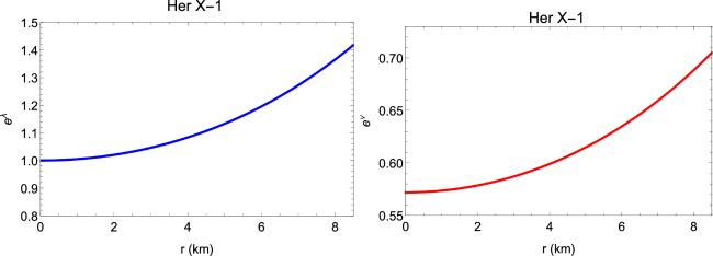
Figure 1. The metric potentials are shown against ‘r'. |
5.2. Density and pressure profiles
Figure 2 shows variations of the energy density, radial pressure, and traverse pressure, respectively, for the α values ranging from 0.5 to 2.5. The plots depicted a monotonically decreasing nature from their maximum values at the center towards the boundary. In the case of radial pressure, it drops to zero, indicating the radius value of the star, while in the case of tangential pressure, it does not zero at the boundary. Also, it is inferred that for higher values of α, density and pressures pick up higher values. ρq decreases with radial parameter and takes more negative as α increases.
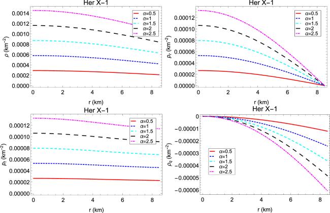
Figure 2. The matter density, radial and transverse pressure are shown for different values of α. |
5.3. Density and pressure gradients
For our current model, we obtain the pressure and density gradient as follows:
$\begin{eqnarray}\displaystyle \frac{{\rm{d}}\rho }{{\rm{d}}r}=-\displaystyle \frac{r({a}^{2}(2+{{Br}}^{2})+a(B+6{{br}}^{2}+3{{bBr}}^{4})+2b(-1+3{{br}}^{4}+B({r}^{2}+{{br}}^{6})))\alpha }{2\pi {\left(1+{{ar}}^{2}+{{br}}^{4}\right)}^{3}(1+\gamma )},\end{eqnarray}$
$\begin{eqnarray}\displaystyle \frac{{\rm{d}}{p}_{r}}{{\rm{d}}r}=-\displaystyle \frac{r({a}^{2}(2+{{Br}}^{2})+a(B+6{{br}}^{2}+3{{bBr}}^{4})+2b(-1+3{{br}}^{4}+B({r}^{2}+{{br}}^{6})))\alpha \gamma }{2\pi {\left(1+{{ar}}^{2}+{{br}}^{4}\right)}^{3}(1+\gamma )},\end{eqnarray}$
$\begin{eqnarray}\begin{array}{l}\displaystyle \frac{{\rm{d}}{p}_{t}}{{\rm{d}}r}=\displaystyle \frac{1}{8\pi {\left(1+{{ar}}^{2}+{{br}}^{4}\right)}^{3}(1+\gamma )}r\alpha \left[-5b-2{B}^{2}(-1+{b}^{2}{r}^{8})(1+\gamma )+{a}^{3}{r}^{2}(1+\gamma )(1+3\omega )\right.\\ -4{{bBr}}^{2}\left(5+4\gamma +3\omega +{{br}}^{4}(1+3\omega )\right)+{a}^{2}\left(5+9\gamma +3\omega +15\gamma \omega +3{{br}}^{4}(1+\gamma )(1+3\omega )-2{{Br}}^{2}(2+\gamma +3\omega )\right)\\ +a\left\{-2{B}^{2}{r}^{2}(-1+{{br}}^{4})(1+\gamma )+{{br}}^{2}\left(13+25\gamma +3\omega +39\gamma \omega +3{{br}}^{4}(1+\gamma )(1+3\omega )\right)-2B\left(4+3\gamma +3\omega \right.\right.\\ \left.\left.\left.+3{{br}}^{4}(2+\gamma +3\omega )\right)\right\}+b\left\{{b}^{2}{r}^{8}(1+\gamma )(1+3\omega )+12{{br}}^{4}\left(1+\gamma (2+3\omega )\right)-3\left(\omega +\gamma (3+5\omega )\right)\right\}\right].\end{array}\end{eqnarray}$
The gradients of density and radial and transverse pressures are shown in figure 3, which are negative inside the stellar structure, which confirms the monotonically decreasing nature of physical parameters from the centre to the boundary.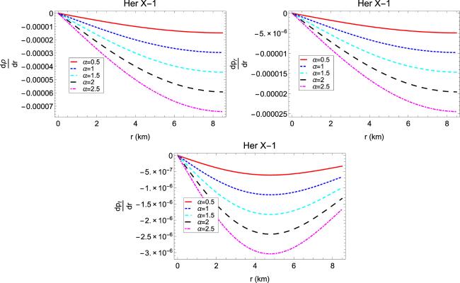
Figure 3. The density and pressure gradient are shown inside the stellar interior. |
5.4. Pressure anisotropy
For our current model, the anisotropic factor Δ is calculated as follows:
$\begin{eqnarray}\begin{array}{l}{\rm{\Delta }}={p}_{t}-{p}_{r}\\ \quad =\displaystyle \frac{1}{32\pi {\left(1+{{ar}}^{2}+{{br}}^{4}\right)}^{2}(1+\gamma )}\left[48\pi \delta -\left\{10{{br}}^{2}\alpha +2{b}^{2}{r}^{6}\alpha +3\beta +6{{br}}^{4}\beta +3{b}^{2}{r}^{8}\beta +34{{br}}^{2}\alpha \gamma +2{b}^{2}{r}^{6}\alpha \gamma \right.\right.\\ \quad \left.+3\beta \gamma +6{{br}}^{4}\beta \gamma +3{b}^{2}{r}^{8}\beta \gamma -4{B}^{2}{r}^{2}(1+{{br}}^{4})\alpha (1+\gamma )\right\}\\ \quad +96\pi {r}^{4}\delta +48{b}^{2}\pi {r}^{8}\delta -3(\beta +\beta \gamma -16\pi \delta )-2{{br}}^{2}\left\{\alpha +5\alpha \gamma \right.\\ \quad \left.+{r}^{2}(\beta +\beta \gamma -16\pi \delta )\right\}-{b}^{2}{r}^{6}\left\{2\alpha (1+\gamma )+{r}^{2}(\beta +\beta \gamma -16\pi \delta )\right\}\omega \\ \quad -6{{ar}}^{2}(1+{{br}}^{4})(\beta +\beta \gamma -16\pi \delta )(1+\omega )\\ \quad +2a\alpha (2{B}^{2}{r}^{4}(1+\gamma )-2{{Br}}^{2}\left\{-2+\gamma -3\omega )-3(1+3\gamma )(1+\omega )-2{{br}}^{4}(1+\gamma )(1+3\omega )\right\}\\ \quad -{a}^{2}{r}^{2}\left\{3{r}^{2}(\beta +\beta \gamma -16\pi \delta )(1+\omega )+2\alpha (1+\gamma )(1+3\omega )\right\}\\ \quad \left.+4B\alpha \left\{3(1+\omega )+{{br}}^{4}(1-2\gamma +3\omega )\right\},],.\right]\end{array}\end{eqnarray}$
The variation of the anisotropy inside the star has been shown in figure 4. The anisotropy is zero at the center since the radial and transverse components are equal as expected and reach their maximum at the surface. Also, it is clear that the anisotropy increases as the α increases.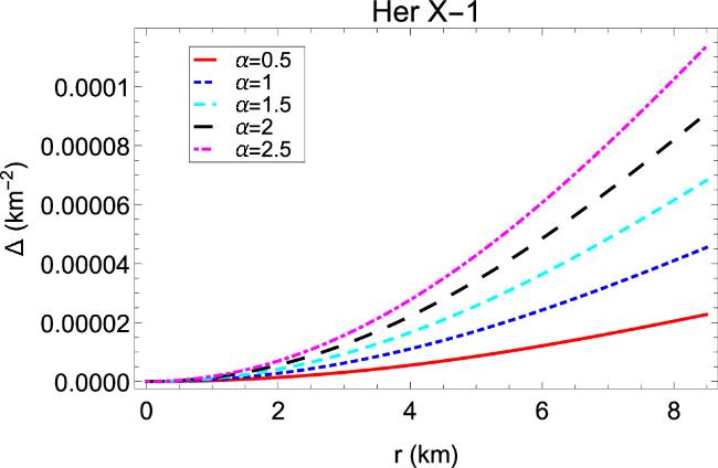
Figure 4. The anisotropic factor is shown for different values of α. |
5.5. Energy conditions
A model representing a physically realistic anisotropic fluid sphere demands satisfaction of the following energy conditions at all internal points, including the surface of the sphere [57]
In figure 5, we have plotted the different energy conditions, and in this model, the necessary energy conditions hold good.
| • | Null energy condition (NEC) : ρ + pr ≥ 0; ρ + pt ≥ 0, |
| • | Weak energy condition (WEC) : ρ + pr ≥ 0; ρ ≥ 0, ρ + pt ≥ 0, |
| • | Strong energy condition (SEC) : ρ + pr ≥ 0; ρ + pr + 2pt ≥ 0, |
| • | Dominant energy condition (DEC) : ρ ≥ 0; ρ − pr ≥ 0; ρ − pt ≥ 0. |
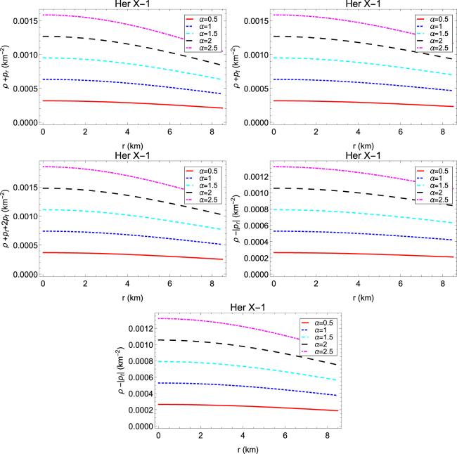
Figure 5. The energy conditions are shown against ‘r'. |
5.6. Equation of state parameters
The equation of state parameters, given by ωr = pr/ρ and ωt = pt/ρ lie within 0 and 1, as depicted in the plot of figure 6. For the matter to be non-exotic in nature, it should satisfy the conditions 0 ≤ ωr ≤ 1 and 0 ≤ ωt ≤ 1, which are ensured by the plot. The expression of ωr and ωt for our present model is given as follows:
$\begin{eqnarray}{\omega }_{r}=\displaystyle \frac{{p}_{r}}{\rho }=\displaystyle \frac{(a+B+(2b+{aB}){r}^{2}+{{bBr}}^{4})\alpha \gamma -4\pi {\left(1+{{ar}}^{2}+{{br}}^{4}\right)}^{2}\delta }{(a+B+(2b+{aB}){r}^{2}+{{bBr}}^{4})\alpha +4\pi {\left(1+{{ar}}^{2}+{{br}}^{4}\right)}^{2}\delta }.\end{eqnarray}$
$\begin{eqnarray}\begin{array}{l}{\omega }_{t}=\displaystyle \frac{{p}_{t}}{\rho }=\displaystyle \frac{(1+3\omega )}{128{\pi }^{2}{\left(1+{{ar}}^{2}+{{br}}^{4}\right)}^{4}(1+\gamma )\left((a+B+(2b+{aB}){r}^{2}+{{bBr}}^{4})\alpha +4\pi {\left(1+{{ar}}^{2}+{{br}}^{4}\right)}^{2}\delta \right)}\\ \quad \times \left[-\beta {\left(1+{{ar}}^{2}+{{br}}^{4}\right)}^{2}-\left\{2\left({a}^{2}{r}^{2}\alpha +2{{abr}}^{4}\alpha \right.\right.\right.\\ \quad +\displaystyle \frac{\alpha \left\{-2B(1+{{br}}^{4})+a(1-2{{Br}}^{2}+3\gamma )+{{br}}^{2}\left(1+5\gamma +{{br}}^{4}(1+\gamma )\right)\right\}-8\pi {\left(1+{{ar}}^{2}+{{br}}^{4}\right)}^{2}\delta }{1+\gamma }+\\ \quad \left.\left.\displaystyle \frac{-2\left\{-a+2B+\left(-2b+B(a+B)\right){r}^{2}+{{aB}}^{2}{r}^{4}+{{bB}}^{2}{r}^{6}\right\}\alpha +{\left(1+{{ar}}^{2}+{{br}}^{4}\right)}^{2}\beta }{1+3\omega }\right\}\right].\end{array}\end{eqnarray}$
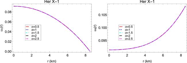
Figure 6. ωr and ωt are shown inside the stellar interior. |
5.7. Stability and equilibrium conditions for our present model
In this section, we are going to discuss the stability and equilibrium conditions of our present model with the help of different criteria.
5.7.1. Causality condition
The causality condition of a stellar model depends on the radial and transverse speeds of sound. The radial and transverse speeds of sound for our present model are obtained as follows,
$\begin{eqnarray}{V}_{r}^{2}=\displaystyle \frac{{\rm{d}}{p}_{r}}{{\rm{d}}\rho }=\gamma ,\end{eqnarray}$
$\begin{eqnarray}\begin{array}{l}{V}_{t}^{2}=\displaystyle \frac{{\rm{d}}{p}_{t}}{{\rm{d}}\rho },\\ =\displaystyle \frac{1}{\left[4\left\{{a}^{2}(2+{{Br}}^{2})+a(B+6{{br}}^{2}+3{{bBr}}^{4})+2b\left(-1+3{{br}}^{4}+B({r}^{2}+{{br}}^{6})\right)\right\}\right]}\\ \quad \left[5b+2{B}^{2}(-1+{b}^{2}{r}^{8})(1+\gamma )-{a}^{3}{r}^{2}(1+\gamma )(1+3\omega )+4{{bBr}}^{2}\left(5+4\gamma +3\omega +{{br}}^{4}(1+3\omega )\right)-{a}^{2}\left(5+9\gamma \right.\right.\\ \quad \left.+3\omega +15\gamma \omega +3{{br}}^{4}(1+\gamma )(1+3\omega )-2{{Br}}^{2}(2+\gamma +3\omega )\right)-a\left\{-2{B}^{2}{r}^{2}(-1+{{br}}^{4})(1+\gamma )+{{br}}^{2}\left(13+25\gamma +3\omega \right.\right.\\ \quad \left.\left.+39\gamma \omega +3{{br}}^{4}(1+\gamma )(1+3\omega )\right)-2B\left(4+3\gamma +3\omega +3{{br}}^{4}(2+\gamma +3\omega )\right)\right\}-b\left({b}^{2}{r}^{8}(1+\gamma )(1+3\omega )\right.\\ \quad \left.\left.\left.-12{{br}}^{4}(1+\gamma (2+3\omega )\right)+3\left(\omega +\gamma (3+5\omega )\right)\right\}\right].\end{array}\end{eqnarray}$
For a physically acceptable stellar model, both the radial and transverse speeds of sound should remain within the limit [0, 1], known as the ‘causality condition'. In figure 7, we have demonstrated the variation of the radial and transverse sound speeds (left panel) with radial parameters. It is found that the sound speeds lie within the prescribed limit, which ensures the non-violation of the causality condition in the interior of the star. Based on Herrera's cracking method [58], Abreau et al [59] set a condition for a potentially stable compact stellar structure that reads $-1\leqslant {V}_{t}^{2}-{V}_{r}^{2}\leqslant 0$. The plot (right panel) confirms this feature of stability.
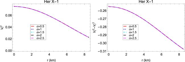
Figure 7. The square of the sound velocity and stability factor ${V}_{t}^{2}-{V}_{r}^{2}$ is shown against r. |
5.7.2. Relatistic adiabatic index
The stability of a relativistic anisotropic stellar configuration is closely related to an important thermodynamical quantity known as the adiabatic index. The adiabatic index, mathematically defined as ${\rm{\Gamma }}=\tfrac{\rho +{p}_{r}}{{p}_{r}}\tfrac{{\rm{d}}{p}_{r}}{{\rm{d}}\rho }$, depends on the EoS and interior fluid density. The stability of an anisotropic fluid sphere is preserved when the adiabatic index >4/3. For our present model, the expression of the relativistic adiabatic index is calculated as follows:
$\begin{eqnarray}\begin{array}{l}{\rm{\Gamma }}\,=\displaystyle \frac{(a+B+(2b+{aB}){r}^{2}+{{bBr}}^{4})\alpha \gamma (1+\gamma )}{(a+B+(2b+{aB}){r}^{2}+{{bBr}}^{4})\alpha \gamma -4\pi {\left(1+{{ar}}^{2}+{{br}}^{4}\right)}^{2}\delta }{V}_{r}^{2},\end{array}\end{eqnarray}$
figure 8 clearly shows that Γ is greater than 4/3 throughout the interior of the star, and hence the stability condition is fulfilled in our model.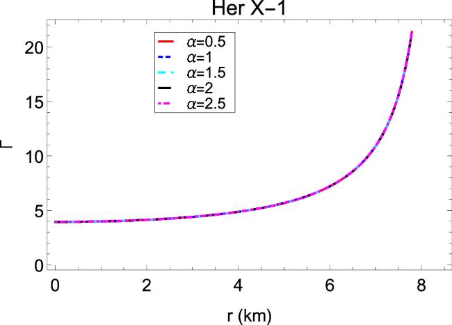
Figure 8. Relativistic adiabatic index is shown inside the stellar interior. |
5.7.3. Equalibrium under three different forces
The stability of an anisotropic star in static equilibrium depends on the different forces, namely, gravitational force (Fg), hydrostatic force (Fh), and anisotropic force (Fa). The anisotropic and hydrostatic forces are directed in a radially outward direction, and strong gravitational forces point inwardly. The condition of balancing the different forces in stable equilibrium is mathematically formulated as a Tolman–Oppenheimer–Volkoff (TOV) equation.
$\begin{eqnarray}-\displaystyle \frac{\nu ^{\prime} }{2}(\rho +{p}_{r})+\displaystyle \frac{2}{r}({p}_{t}-{p}_{r})-\displaystyle \frac{{\rm{d}}{p}_{r}}{{\rm{d}}r}=0,\end{eqnarray}$
which may be rewritten in the form $\begin{eqnarray}{F}_{g}+{F}_{h}+{F}_{a}=0,\end{eqnarray}$
where ${F}_{g}=-\tfrac{\nu ^{\prime} }{2}(\rho +{p}_{r})$, ${Fh}=-\tfrac{{\rm{d}}{p}_{r}}{{\rm{d}}r}$ and ${Fa}=\tfrac{2}{r}({p}_{t}-{p}_{r})$.The nature of these forces is described in figure 9, which shows that all forces increase from the center to attain maximum value at some interior point and then decrease towards the surface. The fact that the sum of all forces vanishes at all interior points results in null, indicating a stable configuration under the combined action of all forces. It is to be noted that the system remains in a static equilibrium condition for different values of α.
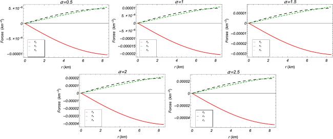
Figure 9. Three different forces acting on the system are shown in the figure for different values of α. |
5.8. Mass, compactness and surface redshift
The mass function of our present model of a quintessence star can be obtained as follows,
$\begin{eqnarray}\begin{array}{l}m(r)={\displaystyle \int }_{0}^{r}4\pi \rho {r}^{2}\,{\rm{d}}r=\displaystyle \frac{1}{1+\gamma }\left[-\displaystyle \frac{r\alpha }{2(1+{{ar}}^{2}+{{br}}^{4})}+\displaystyle \frac{4}{3}\pi {r}^{3}\delta +\right.\\ \quad +\displaystyle \frac{\left(b+(-a+\sqrt{{a}^{2}-4b})B\right)\alpha {\tan }^{-1}\left[\tfrac{\sqrt{2b}r}{\sqrt{a-\sqrt{{a}^{2}-4b}}}\right]}{\sqrt{2b}\sqrt{a-\sqrt{{a}^{2}-4b}}\sqrt{{a}^{2}-4b}}\\ \quad \left.+\displaystyle \frac{\left(-b+(a+\sqrt{{a}^{2}-4b})B\right)\alpha {\tan }^{-1}\left[\tfrac{\sqrt{2b}r}{\sqrt{a+\sqrt{{a}^{2}-4b}}}\right]}{\sqrt{2b}\sqrt{a+\sqrt{{a}^{2}-4b}}\sqrt{{a}^{2}-4b}}\right].\end{array}\end{eqnarray}$
Figure 10 shows the variation of mass, compactness, and surface redshift with radial parameters. The mass function is a monotonically increasing function of r and m(0) = 0, i.e. the mass function is regular at the center. The compactness of a star, which is defined as u(r) = m(r)/r, should lie within a limit as suggested by Buchdahl [60], and the limit for the ratio of mass to the radius is 2M/r < 8/9. For different α plots, it shows that m(r)/r < 4/9 = 0.44, i.e. Buchdahl conditions are satisfied in this model. Surface redshift is defined as
$\begin{eqnarray}z={\left(1-\displaystyle \frac{2M}{R}\right)}^{-1/2}-1.\end{eqnarray}$
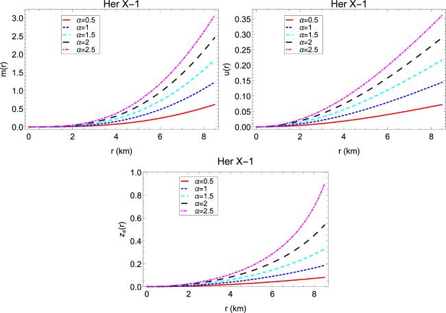
Figure 10. Mass, compactness, and surface redshift are shown inside the stellar interior. |
The variation of z is shown as a radial function in the lower panel of the figure. According to Bohmer and Harko [61], the surface redshift should always be ≤5, which is satisfied in this model for all values of α.
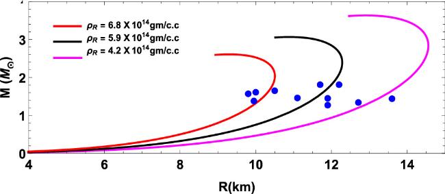
6. Mass-radius relationship
One of the important features of compact stellar modeling is the ability to predict the mass and radius of stars that may exist in nature. One way is to do this by plotting the M−R curve using the TOV equation. In this paper, we have plotted the mass-radius curve with different surface densities for a particular value of α = 0.6 in figure 11. We have also marked the different masses and radii of some observed pulsars [51, 62–66] (KS 1731-260 with M = ${1.61}_{-0.37}^{+0.35}\,{M}_{\odot }$ and R = ${10.0}_{-2.2}^{+2.2}\,\mathrm{km};$ 4U 1608−52 with M = ${1.57}_{-0.29}^{+0.30}\,{M}_{\odot }$ and R = ${9.8}_{-1.8}^{+1.8}\,\mathrm{km};$ EXO 1745−268 with M = ${1.65}_{-0.31}^{+0.21}\,{M}_{\odot }$ and R ${10.5}_{-1.6}^{+1.6}$ km; SAXJ 1748.9−2021 with M = ${1.81}_{-0.37}^{+0.25}\,{M}_{\odot }$ and R = ${11.7}_{-1.7}^{+1.7}\,\mathrm{km};$ 4U 1820 − 30 with M=${1.46}_{-0.21}^{+0.21}\,{M}_{\odot }$ and R = ${11.1}_{-1.8}^{+1.8}\,\mathrm{km};$ 4U 1724 − 207 with M = ${1.81}_{-0.37}^{+0.25}\,{M}_{\odot }$ and R ${12.2}_{-1.4}^{+1.4}\,\mathrm{km};$ M13 with M = ${1.38}_{-0.23}^{+0.08}\,{M}_{\odot }$ and R ${9.95}_{-0.27}^{+0.24}\,\mathrm{km};$ J0030 + 0451 with M = ${1.34}_{-0.16}^{+0.15}\,{M}_{\odot }$ and R = ${12.71}_{-1.19}^{+1.14}\,\mathrm{km};$ J0437−4715 with M = ${1.44}_{-0.07}^{+0.07}\,{M}_{\odot }$ and R = ${13.6}_{-0.8}^{+0.9}\,\mathrm{km};$ GW 170817−1 with M ${1.45}_{-0.09}^{+0.09}\,{M}_{\odot }$ and R = ${11.9}_{-1.4}^{+1.4}\,\mathrm{km};$ GW 170817−2 with M ${1.27}_{-0.09}^{+0.09}\,{M}_{\odot }$ and R = ${11.9}_{-1.4}^{+1.4}\,\mathrm{km}$) with their recent data in the plot. The observed values corresponding to mass and radius are found to fit in the M−R curve. The plot also predicts the possibility of the existence of higher mass for a certain range of boundary surface density.
Figure 11. The mass-radius curve for three different surface densities along with mass-radius points of some observed pulsars. |
7. Discussion
Within the context of f(T) gravity theory, we developed an analytical relativistic anisotropic quintessence spherical model in the current paper. Three ingredients, which serve as the main pillars of the resulting paradigm, were imposed to achieve this. The first of them was to take into account a straightforward, noteworthy, and realistic modified gravity model given by f(T) = αT + β, where T is the torson, α is a coupling constant, and β is another constant. The second step is to choose the metric coefficients, and for this task, we have opted to use the coefficients that TK has suggested. The matter density and radial pressure possess a linear equation of state-imposed between them. We have effectively generated the expressions for matter density, radial and transverse pressure, as well as the matter density associated with the quintessence field, using these components. Once that was done, we continued to obtain the constant parameters of the solution. We developed a matching between the internal and external Schwarzschild solutions at the boundary of the compact structure for this purpose. In terms of the mass and radius of the compact star, we were able to successfully acquire various model parameters by using the matching conditions. The existence, stability, and equilibrium of spherical stars in the f(T) theory are the next topics of interest to us. We have investigated the behavior of the key distinguishing characteristics for this purpose, including the radial and tangential pressure, matter density, and anisotropy factor. Both the parameter ω and the parameter α have an impact on the model parameters, which will be summarized here. Throughout the analysis, we have taken a wide range of α, i.e. for the plotting of the model parameters, we have chosen α ∈ [0, 2.5].
Central density, surface density, central pressure, compactness factor, and surface redshift have been presented for the compact star Her X-1 for different values of α in table 2. According to our findings, all three thermodynamic observables ρ, pr, and pt remain positive and reach their highest values at the core of the compact star. This indicates that they behave monotonically, decreasing from the center to the boundary. It is interesting to see that ρ, pr, and pt have higher central values when α = 2.5 is applied; however, these values are lower when α = 0.5. For all chosen values of α, the anisotropic factor Δ is a positive and monotonic increasing function throughout the object. In order to prevent point singularities or the creation of a black hole, a positive anisotropy factor signifies that the system is subject to an external repulsive force that works to balance the gravitational attraction. For all values of α, in this investigation, the energy conditions are valid. Since the material inside the object cannot travel faster than light, our current model satisfies the constraints of causality. The profiles of Vt2 coincide for all values of α, as seen in figure 7. It has been discovered that the range [0, 1] encompasses the difference between the squares of the subliminal sound speeds, i.e. $| {V}_{t}^{2}-{V}_{r}^{2}| \in [0,1]$. Figure 10 illustrates the maximum feasible value of the surface redshift, which cannot be arbitrarily large. The compactness factor for our current model is below the maximum value found in the literature, i.e. $u{| }_{\max }\lt 4/9$. The TOV equation is used to study the analysis of the balance mechanism in the context of the f(T) model. It is demonstrated that the system is subject to three forces for the specific choice of the f(T) model, namely the hydrostatic force Fh, gravitational force Fg, and anisotropic force Fa, achieving the equilibrium condition by maintaining the sum of all the forces to be zero. Additionally, we have shown the equation of the state parameters ωr and ωt for all values of α, and for our current model, the profiles of ωr and ωt coincide for all values of α. It should be mentioned that ωr and ωt both fall within the range [0, 1]. For our current model, the maximum permissible mass and associated radius were determined using the M−R curve, and they are shown in figure 11. A comprehensive graphical analysis is used to support each of the concepts shown in figures 1–11. In conclusion, the models we have described here meet all the physical requirements, making them perfect choices to represent reliable models in the context of f(T) gravity.