


1. Introduction
Since the first successful detection of gravitational waves in 2015, about 100 gravitational wave events have been reported. All these events are found by matched filtering techniques. To date, the matched filtering technique is still the standard data analysis method for gravitational wave detection [1, 2]. As expected, the situation will also be true for space-based detectors in the near future [3, 4].
To enable the matched filtering technique to work, accurate and complete waveform templates are needed [5–8]. Besides the above-mentioned matched filtering method, there is a time-frequency excess power identification method [9]. However, if an accurate waveform is available and can aid the analysis, the method will become more efficient [10]. In addition, the machine learning method is a new technique that is used to treat gravitational wave data [11–16]. A data set that consists of a large amount of gravitational wave samples is critically important to enable the machine learning method to work well. Since real gravitational wave events are too few to play the role of such a data set, accurate waveform templates are needed. In short, no matter what kind of data analysis means are used, waveform templates are very important to gravitational wave data analysis.
A waveform template means the accurate waveform with respect to time or frequency when a set of source parameters are specified. Specifically, a waveform template is only valid for a class of source that falls in a specified parameter range. Until now, the gravitational wave astronomy community has only understood binary compact object systems well. Consequently, only waveform templates of binary systems are currently available. This fact also explains, to some extent, why only events of the coalescence of binary objects have been observed until now. In contrast, the current detection ability for supernovae gravitational waves is quite weak [17]. Roughly, the detection horizon is just 1kpc (figure 5(a) of [17]). The partial reason for such a fact is the lack of an accurate waveform template for supernovae gravitational waves.
Before the breakthrough of numerical relativity [18–22], the waveform template problem was treated mainly via post-Newtonian approximation [23]. As an enhanced post-Newtonian approximation method, the effective-one-body theory shows better convergent behavior [24]. After the success of numerical relativity simulation of a binary black hole merger, the complete inspiral-merger-ringdown behavior is revealed. The power of effective-one-body theory to describe the waveform of coalescence of a binary object is verified [25]. Following this, numerical relativity waveforms are extensively used to construct waveform templates for the coalescence of binary objects.
To date, there are a bundle of waveform templates for the coalescence of binary objects available in the laser interferometer gravitational wave observatory (LIGO) data analysis software. Among the types of waveform template models, including the EOBNR series [26–31], IMRphenom series [32, 33] and numerical relativity surrogate models [34–36], the numerical relativity waveforms are bases for the waveform template construction. When people talk about the accuracy of a waveform model, numerical relativity waveforms are treated as the standard answer. Therefore, the accuracy of numerical relativity waveforms themselves is critically important to waveform template construction.
Both ground-based and space-based gravitational wave detectors utilize matched filtering techniques for the detection of gravitational waves. Therefore, when calculating the accuracy of the templates, the formulas used are very similar to those of the matched filtering technique. Consideration of the detector noise is crucial when using the matched filtering technique to search for signals. Hence, when calculating the accuracy of the waveform templates, it is necessary to take into account the sensitivity of different detectors. The noise characteristics of space-based gravitational wave detectors differ significantly from those of ground-based detectors. Therefore, the purpose of this article is to investigate whether the numerical relativity waveform's accuracy can meet the requirements of space-based detectors. When one discusses the accuracy of a waveform model, a specific detector should be referred to. The accuracy issue of numerical relativity waveforms has been extensively studied against advanced LIGO detectors [37]. However, this issue has not been investigated against space-based detectors. The current paper aims to conduct such an investigation and lays down a foundation of waveform template construction for space-based detectors.
In the next section we introduce the waveform accuracy estimation method. Next, we apply the method in section 3 to calculate the waveform accuracy of the waveforms of the SXS numerical relativity catalog. LISA, Taiji and Tianqin detectors are all considered. Finally, a summary and conclusion are given in the last section.
2. Matching factor and accuracy indicator
Following the idea of the matched filtering data analysis method, a matching factor has been extensively used to quantify how close two given waveforms are to each other. With respect to a detector sensitivity S(f), which describes the one sided power spectrum of the detector noise, the matching factor of two real waveforms h1(t) and h2(t) can be expressed as
$\begin{eqnarray}\mathrm{FF}\equiv \mathop{\max }\limits_{t}\displaystyle \frac{\langle {h}_{1}| {h}_{2}\rangle }{\parallel {h}_{1}\parallel \cdot \parallel {h}_{2}\parallel },\end{eqnarray}$
$\begin{eqnarray}\langle {h}_{1}| {h}_{2}\rangle =2{\int }_{{f}_{\mathrm{low}}}^{{f}_{\mathrm{up}}}\displaystyle \frac{{\tilde{h}}_{1}{\tilde{h}}_{2}^{* }+{\tilde{h}}_{1}^{* }{\tilde{h}}_{2}}{S(f)}{\rm{d}}{f},\end{eqnarray}$
$\begin{eqnarray}\parallel h\parallel \equiv \sqrt{\langle h| h\rangle },\end{eqnarray}$
where the ‘$\tilde{(\cdot )}$' means the Fourier transformation, the ‘*' means taking the complex conjugate, and the maximum is taken with respect to the time shift to align the two waveforms (flow, fup) and corresponds to the frequency band where the two waveforms should be compared. Within PyCBC software [38], the command line ‘pycbc.filter.matchedfilter.match' can be used to do the above calculation of the matching factor FF. Together with the value of the matching factor, the time shift is also returned by the command line.For a theoretical waveform template, two polarization waveforms will be given, h+(t) and h×(t). Usually, people are used to the complex waveform defined as1 ) can be defined to quantify the closeness between two complex waveforms. The only difference to equation (1 ) is that the maximum should be taken with respect to the initial phase besides the shifted time. The initial phase describes the phase difference between the two polarization modes h+(t) and h×(t) at the initial time.
$\begin{eqnarray}h\equiv {h}_{+}-{{ih}}_{\times }.\end{eqnarray}$
Then, a similar matching factor to equation (Assume we have two complex waveforms h1,2 = h1,2+ − ih1,2×; the linearity of the inner product, equation (2 ), results in2 ) can be equivalently expressed as
$\begin{eqnarray}\begin{array}{l}\langle {h}_{1}| {h}_{2}\rangle =\langle {h}_{1+}| {h}_{2+}\rangle +\langle {h}_{1\times }| {h}_{2\times }\rangle \\ \,-\ i\langle {h}_{1+}| {h}_{2\times }\rangle -i\langle {h}_{1\times }| {h}_{2+}\rangle .\end{array}\end{eqnarray}$
Meanwhile, equation ( $\begin{eqnarray}\langle {h}_{1}| {h}_{2}\rangle =4{\mathfrak{R}}\int \displaystyle \frac{{\tilde{h}}_{1}{\tilde{h}}_{2}^{* }}{S(f)}{\rm{d}}{f},\end{eqnarray}$
where ${\mathfrak{R}}$ means taking the real part. Therefore, we have $\begin{eqnarray}\langle {h}_{1}| {h}_{2}\rangle =\langle {h}_{1+}| {h}_{2+}\rangle +\langle {h}_{1\times }| {h}_{2\times }\rangle ,\end{eqnarray}$
which corresponds to $\begin{eqnarray}\mathop{\max }\limits_{t,\phi }\langle {h}_{1}| {h}_{2}\rangle =\mathop{\max }\limits_{{t}_{+}}\langle {h}_{1+}| {h}_{2+}\rangle +\mathop{\max }\limits_{{t}_{\times }}\langle {h}_{1\times }| {h}_{2\times }\rangle .\end{eqnarray}$
Here, t means the time shift for the complex waveform, φ means the initial phase difference of the two polarization modes, and t+,× are the time shifts for the two polarization waveforms. Due to the above relations, we have $\begin{eqnarray}\mathrm{FF}=\displaystyle \frac{{\mathrm{FF}}_{+}\parallel {h}_{1+}\parallel \cdot \parallel {h}_{2+}\parallel +{\mathrm{FF}}_{\times }\parallel {h}_{1\times }\parallel \cdot \parallel {h}_{2\times }\parallel }{\parallel {h}_{1}\parallel \cdot \parallel {h}_{2}\parallel },\end{eqnarray}$
$\begin{eqnarray}{\mathrm{FF}}_{+}\equiv \mathop{\max }\limits_{t}\displaystyle \frac{\langle {h}_{1+}| {h}_{2+}\rangle }{\parallel {h}_{1+}\parallel \cdot \parallel {h}_{2+}\parallel },\end{eqnarray}$
$\begin{eqnarray}{\mathrm{FF}}_{\times }\equiv \mathop{\max }\limits_{t}\displaystyle \frac{\langle {h}_{1\times }| {h}_{2\times }\rangle }{\parallel {h}_{1\times }\parallel \cdot \parallel {h}_{2\times }\parallel }.\end{eqnarray}$
Basically, we can calculate the matching factors FF+ and FF× for two polarization modes individually, and then use the above equation to combine the final matching factor we wanted. In the current work we follow this method and use the PyCBC tool to calculate the matching factor.Similarly to any other computing science topics, the only errors involved in numerical relativity include truncation errors and round-off errors. Truncation errors are due to the numerical approximation of derivatives. Round-off errors are due to the memory limit of computers. In practice, one needs to make sure the real calculation is dominated by truncation errors. Consequently, the final error related to the numerical solution is proportional to a power of the resolution used in the numerical calculation. The power index is nothing but the convergence order of the involved numerical algorithm. Therefore, we can use the difference between the results of two different resolutions to quantitatively estimate the error of the numerical solution.
3. Accuracy of numerical relativity waveforms
3.1. Fourier transforms of numerical relativity waveforms
Numerical relativity waveforms are presented in the time domain. To calculate the matching factor explained in the last section, we need to transform these waveforms to the frequency domain. In practice, we use fast Fourier transformation to get the waveforms in the frequency domain.
To reduce the Gibbs effect and spectral leakage resulting from truncation in the time domain, we apply the Plank window ΣT(t) to the time domain waveform before the Fourier transformation. The Plank window ΣT(t) is set as [40, 41]
$\begin{eqnarray}\sigma (t)=\left\{\begin{array}{lr}0, & t\lt {t}_{1}\\ {\sigma }_{\mathrm{start}\ }(t), & {t}_{1}\leqslant t\lt {t}_{2}\\ 1, & {t}_{2}\leqslant t\lt {t}_{3}\\ {\sigma }_{\mathrm{end}\ }(t), & {t}_{3}\leqslant t\lt {t}_{4}\\ 0, & {t}_{4}\leqslant t\end{array}\right.\end{eqnarray}$
where Σstart is the segment that smoothly increases from 0 to 1 between t1 and t2 , and Σend is the segment that smoothly decreases from 1 to 0 between t3 and t4: $\begin{eqnarray}\begin{array}{l}{\sigma }_{\mathrm{start}\ }(t)={\left[\exp \left(\displaystyle \frac{{t}_{2}-{t}_{1}}{t-{t}_{1}}+\displaystyle \frac{{t}_{2}-{t}_{1}}{t-{t}_{2}}\right)+1\right]}^{-1},\\ {\sigma }_{\mathrm{end}\ }(t)={\left[\exp \left(\displaystyle \frac{{t}_{3}-{t}_{4}}{t-{t}_{3}}+\displaystyle \frac{{t}_{3}-{t}_{4}}{t-{t}_{4}}\right)+1\right]}^{-1}.\end{array}\end{eqnarray}$
Then, we further zero pad the waveform to the nearest power of 2.3.2. Frequency range of numerical relativity waveforms
Typically, we get waveforms in the frequency domain like the one shown in figure 1. Apparently, only the part between the two vertical dashed lines is reliable. The left vertical line corresponds to the lowest frequency ${f}_{\min }$ of the numerical relativity waveform, which is determined by the length of the waveform. The right vertical line corresponds the highest frequency ${f}_{\max }$, where the numerical error begins to dominate.
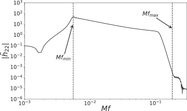
Figure 1. The frequency waveform of SXS:BBH:2106. This waveform corresponds to a quasi-circular coalescing binary black hole system with mass ratio 1, dimensionless spin ${\vec{\chi }}_{1}=(0,0,0.8998)$ and ${\vec{\chi }}_{2}=(0,0,0.5)$. In the plot, M means the total mass of the binary. The horizontal axis has no special meaning. It just indicates different numerical relativity simulations. |
There are 1872 waveforms in the SXS catalog [39] that have more than one resolution result. In figures 2(a) and (b), we plot ${{Mf}}_{\min }$ and ${{Mf}}_{\max }$ of these waveforms Here, M means the total mass of the binary system. Different numerical relativity waveforms begin at different frequencies corresponding to ${{Mf}}_{\min }$. ${{Mf}}_{\min }$ ranges from about 0.002 to 0.012. Most waveforms admit ${{Mf}}_{\min }\approx 0.006$. A lower ${{Mf}}_{\min }$ means the corresponding binary system begins at larger separation and the waveform is longer. Roughly, ${{Mf}}_{\max }$ falls in the quasi-normal mode stage. The specific value of ${{Mf}}_{\max }$ depends on the specific numerical simulation. From the viewpoint of the resolution requirement of the binary system in question, if the numerical resolution is higher, the value of ${{Mf}}_{\max }$ is larger. Relatively, the numerical setting is random; therefore, the behavior of ${{Mf}}_{\max }$ shown in figure 2(b) is random.
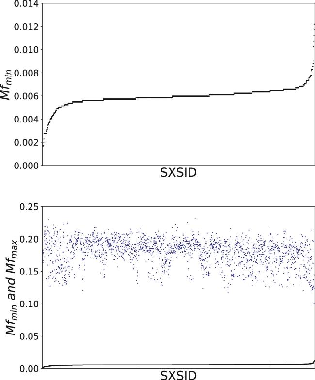
Figure 2. The frequency lower and upper limit of the 1872 numerical relativity waveforms in the SXS catalog. The top panel is the lower limit ${{Mf}}_{\min }$. The bottom panel shows both the lower limit (black dots) and the upper limit (blue dots). |
3.3. Accuracy of numerical relativity waveforms with respect to LIGO
For comparison convenience, we also investigate the accuracy of numerical relativity waveforms with respect to LIGO detectors. Specifically, we use the designed sensitivity of advanced LIGO [42]. The frequency band of LIGO is (10, 8192) Hz.
Note that only the numerical relativity waveform falling in the range $({{Mf}}_{\min },{{Mf}}_{\max })$ is trustable. By considering the source character for LIGO, we investigate M ∈ (10, 200) M⊙. In figure 3, we show the trustable frequency range for a binary system with total mass M = 10 M⊙. For other total mass systems we need to only rescale the vertical axis that is proportional to the inverse of the system total mass 1/M. In figure 3(a) we can see clearly that the numerical relativity simulation cannot cover the whole frequency range of LIGO detection. This is due to the well-known expensive computational cost of numerical relativity. Consequently, numerical relativity only starts near merger. For the early inspiral part, people rely on post-Newtonian approximation to construct the waveform template. In the current work, we just care about the accuracy of numerical relativity; therefore, we take the integrand bound in equation (2 ) as
$\begin{eqnarray}{f}_{\mathrm{low}}=\max (10,{f}_{\min }),\end{eqnarray}$
$\begin{eqnarray}{f}_{\mathrm{up}}=\min (8192,{f}_{\max }).\end{eqnarray}$
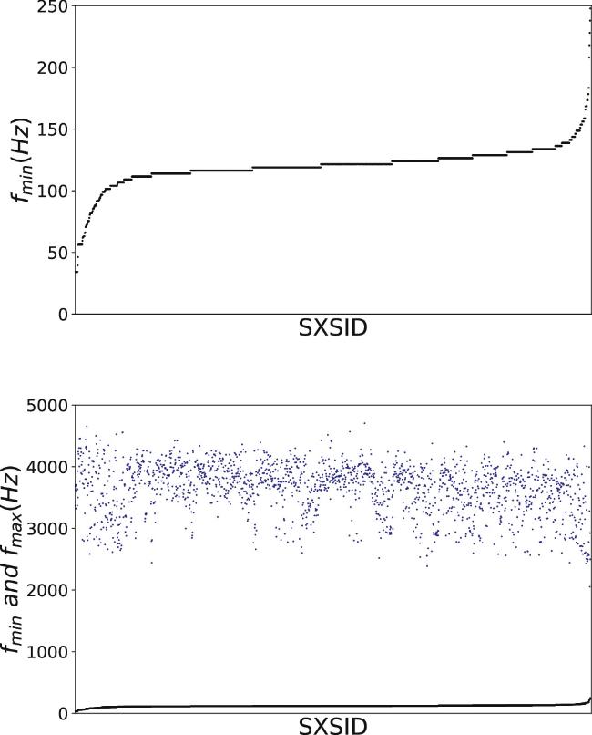
Figure 3. The trustable frequency range of numerical relativity waveforms of the 1872 numerical relativity waveforms in the SXS catalog for the M = 10 M⊙ binary system. The top plot is the lower limit ${{Mf}}_{\min }$. The bottom plot shows both the lower limit (black dots) and the upper limit (blue dots). |
In the first panel of figure 4 we plot the mismatch factors
$\begin{eqnarray}{ \mathcal M }\equiv 1-\mathrm{FF}\end{eqnarray}$
with respect to LIGO between the highest resolution simulation and the second-highest resolution simulation.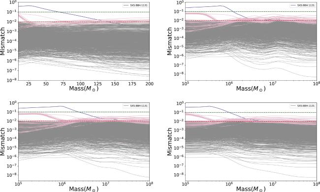
Figure 4. The mismatch factors between the highest resolution simulation and the second-highest resolution simulation. All 1872 SXS waveforms are investigated here. From top to bottom, from left to right the subfigures correspond to LIGO, LISA, Taiji and Tianqin, respectively. The blue lines in all of the subfigures correspond to SXS:BBH:1131. |
3.4. Accuracy of numerical relativity waveforms with respect to space-based detectors
Specifically, we use the following approximated sensitivity for space-based gravitational wave detectors (equation (13 ) of [48])
$\begin{eqnarray}\begin{array}{rcl}{S}_{n}(f) & = & \displaystyle \frac{10}{3{L}^{2}}\left({P}_{\mathrm{OMS}}+2(1+{\cos }^{2}(f/{f}_{* }))\displaystyle \frac{{P}_{\mathrm{acc}}}{{\left(2\pi f\right)}^{4}}\right)\\ & & \times \ \left(1+\displaystyle \frac{6}{10}{\left(\displaystyle \frac{f}{{f}_{* }}\right)}^{2}\right),\end{array}\end{eqnarray}$
$\begin{eqnarray}{f}_{* }=c/(2\pi L).\end{eqnarray}$
For LISA [48] we have $\begin{eqnarray}{P}_{\mathrm{OMS}}={\left(1.5\times {10}^{-11}{\rm{m}}\right)}^{2}{\mathrm{Hz}}^{-1},\end{eqnarray}$
$\begin{eqnarray}{P}_{\mathrm{acc}}={\left(3\times {10}^{-15}{\mathrm{ms}}^{-2}\right)}^{2}\left(1+{\left(\displaystyle \frac{4\times {10}^{-4}\mathrm{Hz}}{f}\right)}^{2}\right){\mathrm{Hz}}^{-1},\end{eqnarray}$
$\begin{eqnarray}L=2.5\,\times \,{10}^{9}{\rm{m}}.\end{eqnarray}$
For Taiji [49] we have $\begin{eqnarray}{P}_{\mathrm{OMS}}={\left(8\times {10}^{-12}{\rm{m}}\right)}^{2}{\mathrm{Hz}}^{-1},\end{eqnarray}$
$\begin{eqnarray}{P}_{\mathrm{acc}}={\left(3\times {10}^{-15}{\mathrm{ms}}^{-2}\right)}^{2}\left(1+{\left(\displaystyle \frac{4\times {10}^{-4}\mathrm{Hz}}{f}\right)}^{2}\right){\mathrm{Hz}}^{-1},\end{eqnarray}$
$\begin{eqnarray}L=3\times {10}^{9}{\rm{m}}.\end{eqnarray}$
For Tianqin we have [45] $\begin{eqnarray}{P}_{\mathrm{OMS}}={\left(1\times {10}^{-12}{\rm{m}}\right)}^{2}{\mathrm{Hz}}^{-1},\end{eqnarray}$
$\begin{eqnarray}{P}_{\mathrm{acc}}={\left(1\times {10}^{-15}{\mathrm{ms}}^{-2}\right)}^{2}\left(1+{\left(\displaystyle \frac{1\times {10}^{-4}\mathrm{Hz}}{f}\right)}^{2}\right){\mathrm{Hz}}^{-1},\end{eqnarray}$
$\begin{eqnarray}L=\sqrt{3}\times {10}^{8}{\rm{m}}.\end{eqnarray}$
Besides the instrument noise mentioned above, there is more confusion noise due to the Galaxy binaries, which can be approximated as [50]
$\begin{eqnarray}\begin{array}{rcl}{S}_{c}(f) & = & {{Af}}^{-7/3}{{\rm{e}}}^{-{f}^{\alpha }+\beta f\sin (\kappa f)}\\ & & \times \ \left[1+\tanh \left(\gamma \left({f}_{k}-f\right)\right)\right]{\mathrm{Hz}}^{-1}\end{array}\end{eqnarray}$
$\begin{eqnarray}A=9\,\times \,{10}^{-45},\end{eqnarray}$
$\begin{eqnarray}\alpha =0.133,\end{eqnarray}$
$\begin{eqnarray}\beta =243,\end{eqnarray}$
$\begin{eqnarray}\kappa =482,\end{eqnarray}$
$\begin{eqnarray}\gamma =917,\end{eqnarray}$
$\begin{eqnarray}{f}_{k}=0.00258.\end{eqnarray}$
Note that parameters α, β, κ, γ depend on observation time. The values listed above correspond to an observation time of half a year. The overall noise sensitivity of space-based detectors can be estimated as $\begin{eqnarray}S={S}_{n}+{S}_{c}.\end{eqnarray}$
Due to the similar reason for LIGO, we take the integrand bound in equation (2 ) as
$\begin{eqnarray}{f}_{\mathrm{low}}=\max ({10}^{-5},{f}_{\min }),\end{eqnarray}$
$\begin{eqnarray}{f}_{\mathrm{up}}=\min (1,{f}_{\max }),\end{eqnarray}$
for space-based detectors.Numerical relativity waveforms have a critical limitation in that they are somewhat short (due to the computational cost) and mainly focus on the merger phase. In particular, for the gravitational waves emitted by supermassive black hole binaries, the majority of the evolution occurs in the inspiral phase. Therefore, simply calculating the accuracy of numerical relativity waveforms will lose the important inspiral phase, which will affect the results of the accuracy of the waveforms. In future work, we plan to use the post-Newtonian numerical relativity waveform models, including SEOBNR, SEOBNRE and others, to investigate the waveform template accuracy for space-based detectors.
The corresponding mismatch factors between the highest resolution simulation and the second-highest resolution simulation for LISA, Taiji and Tianqin are shown in figure 4. Similar to the situation for LIGO, most numerical relativity simulations admit accuracy better than 99%. A few numerical relativity simulations have less accuracy. We list these less accurate simulations in table 1.
Table 1. Less accurate (${ \mathcal M }\gt 1 \% $) numerical relativity simulations found in this work. Here, we list the parameters for each simulation, including the mass ratio q, lowest frequency ${{Mf}}_{\min }$, highest frequency ${{Mf}}_{\max }$ and initial spin configuration. Additionally, we provide the maximum mismatch between the highest resolution simulation and the second-highest resolution simulation $\max { \mathcal M }$. Here, max means the maximum value in the total mass range shown in figure 4. The subscriptions ‘LIGO', ‘LISA', ‘Taiji' and ‘Tianqin' are for corresponding detectors. |
| SXS ID | q | χ1 | χ2 | ${{Mf}}_{\min }$ | ${{Mf}}_{\max }$ | $\max {{ \mathcal M }}_{\mathrm{LIGO}}$ | $\max {{ \mathcal M }}_{\mathrm{LISA}}$ | $\max {{ \mathcal M }}_{\mathrm{Taiji}}$ | $\max {{ \mathcal M }}_{\mathrm{Tianqin}}$ |
|---|---|---|---|---|---|---|---|---|---|
| 1415 | 1.50 | (0.00,0.00,0.50) | (0.00,−0.00,0.50) | 0.0017 | 0.1789 | 0.0756 | 0.0978 | 0.1005 | 0.1077 |
| 0627 | 1.91 | (−0.51,0.44,−0.35) | (0.19,−0.01,−0.06) | 0.0083 | 0.1626 | 0.0709 | 0.0650 | 0.0660 | 0.0491 |
| 1413 | 1.41 | (−0.00,−0.00,0.50) | (−0.00,−0.00,0.40) | 0.0017 | 0.1660 | 0.0570 | 0.0732 | 0.0755 | 0.0805 |
| 1414 | 1.83 | (−0.00,−0.00,−0.50) | (0.00,−0.00,0.40) | 0.0017 | 0.1636 | 0.0527 | 0.0695 | 0.0715 | 0.0749 |
| 1390 | 1.42 | (0.15,0.44,−0.16) | (−0.02,0.34,0.10) | 0.0017 | 0.1659 | 0.0510 | 0.0648 | 0.0672 | 0.0714 |
| 1393 | 1.79 | (−0.37,−0.33,−0.00) | (−0.27,−0.39,0.11) | 0.0017 | 0.1784 | 0.0490 | 0.0647 | 0.0667 | 0.0694 |
| 1392 | 1.51 | (−0.40,0.23,0.17) | (0.35,−0.13,−0.25) | 0.0017 | 0.1795 | 0.0478 | 0.0625 | 0.0642 | 0.0679 |
| 1389 | 1.63 | (−0.29,0.20,−0.30) | (−0.01,0.42,0.16) | 0.0017 | 0.1771 | 0.0460 | 0.0594 | 0.0613 | 0.0651 |
| 1391 | 1.83 | (−0.15,0.29,−0.33) | (−0.33,−0.29,−0.03) | 0.0017 | 0.1813 | 0.0440 | 0.0566 | 0.0583 | 0.0619 |
| 1412 | 1.63 | (−0.00,−0.00,0.40) | (−0.00,0.00,−0.30) | 0.0017 | 0.1822 | 0.0421 | 0.0562 | 0.0578 | 0.0606 |
| 1416 | 1.78 | (0.00,−0.00,−0.40) | (−0.00,0.00,−0.40) | 0.0017 | 0.1825 | 0.0392 | 0.0524 | 0.0539 | 0.0561 |
| 1926 | 4.00 | (0.76,0.26,0.04) | (0.00,−0.14,0.79) | 0.0065 | 0.1943 | 0.0266 | 0.0350 | 0.0337 | 0.0335 |
| 2000 | 4.00 | (−0.40,0.69,0.08) | (0.45,0.65,−0.11) | 0.0066 | 0.1902 | 0.0171 | 0.0206 | 0.0204 | 0.0204 |
| 1992 | 4.00 | (−0.61,0.07,−0.51) | (−0.27,0.75,−0.05) | 0.0062 | 0.1733 | 0.0162 | 0.0192 | 0.0195 | 0.0194 |
| 2044 | 4.00 | (0.74,−0.29,0.11) | (0.14,−0.60,0.52) | 0.0067 | 0.1890 | 0.0148 | 0.0151 | 0.0149 | 0.0140 |
| 1991 | 4.00 | (−0.26,−0.51,−0.56) | (−0.07,0.06,0.79) | 0.0061 | 0.1724 | 0.0136 | 0.0201 | 0.0219 | 0.0221 |
| 2038 | 4.00 | (−0.80,−0.05,0.05) | (−0.01,−0.08,−0.39) | 0.0065 | 0.1920 | 0.0135 | 0.0249 | 0.0244 | 0.0246 |
| 2054 | 4.00 | (0.66,−0.45,0.08) | (0.38,−0.31,0.63) | 0.0065 | 0.1887 | 0.0135 | 0.0199 | 0.0190 | 0.0192 |
| 2074 | 4.00 | (−0.66,0.44,0.07) | (−0.74,0.28,0.10) | 0.0066 | 0.1548 | 0.0127 | 0.0214 | 0.0210 | 0.0211 |
| 1987 | 4.00 | (0.38,0.43,−0.55) | (0.54,0.58,0.04) | 0.0062 | 0.1659 | 0.0119 | 0.0160 | 0.0177 | 0.0182 |
| 1110 | 7.00 | (−0.00,−0.00,0.00) | (−0.00,−0.00,−0.00) | 0.0023 | 0.1724 | 0.0106 | 0.0510 | 0.0423 | 0.0427 |
| 1928 | 4.00 | (−0.33,0.72,0.07) | (0.62,0.48,−0.13) | 0.0065 | 0.1898 | 0.0104 | 0.0114 | 0.0115 | 0.0113 |
| 1978 | 4.00 | (0.50,0.26,0.57) | (−0.77,−0.20,0.03) | 0.0070 | 0.1438 | 0.0092 | 0.0171 | 0.0168 | 0.0179 |
| 1135 | 1.00 | (−0.00,−0.00,−0.44) | (−0.00,0.00,−0.44) | 0.0073 | 0.1355 | 0.0089 | 0.0134 | 0.0137 | 0.0097 |
| 1623 | 3.93 | (0.02,0.55,0.43) | (−0.56,−0.33,−0.45) | 0.0066 | 0.1863 | 0.0089 | 0.0187 | 0.0184 | 0.0176 |
| 1993 | 4.00 | (−0.06,−0.58,−0.54) | (−0.24,−0.76,0.02) | 0.0062 | 0.1439 | 0.0087 | 0.0109 | 0.0116 | 0.0121 |
| 1994 | 4.00 | (0.58,0.16,−0.53) | (0.11,−0.79,−0.08) | 0.0062 | 0.1938 | 0.0085 | 0.0121 | 0.0118 | 0.0108 |
| 1981 | 4.00 | (0.26,−0.55,−0.52) | (−0.35,−0.72,−0.02) | 0.0062 | 0.1460 | 0.0081 | 0.0120 | 0.0114 | 0.0101 |
| 1156 | 4.39 | (−0.16,0.21,0.38) | (0.53,−0.55,0.11) | 0.0041 | 0.1776 | 0.0079 | 0.0085 | 0.0088 | 0.0106 |
| 1629 | 3.46 | (0.54,0.15,−0.45) | (−0.23,0.08,−0.73) | 0.0059 | 0.2096 | 0.0077 | 0.0089 | 0.0097 | 0.0104 |
| 1923 | 4.00 | (−0.79,0.04,0.09) | (−0.75,0.28,0.02) | 0.0066 | 0.1622 | 0.0074 | 0.0188 | 0.0184 | 0.0169 |
| 2011 | 4.00 | (0.79,−0.09,0.03) | (0.37,0.69,0.18) | 0.0063 | 0.2168 | 0.0064 | 0.0292 | 0.0260 | 0.0243 |
| 1863 | 3.63 | (−0.45,0.30,−0.58) | (0.33,0.33,0.43) | 0.0060 | 0.1654 | 0.0063 | 0.0114 | 0.0133 | 0.0137 |
| 1997 | 4.00 | (−0.76,−0.24,0.04) | (−0.00,0.14,0.79) | 0.0063 | 0.1663 | 0.0060 | 0.0114 | 0.0104 | 0.0101 |
| 1983 | 4.00 | (−0.47,0.35,−0.55) | (−0.52,−0.59,0.14) | 0.0062 | 0.1721 | 0.0058 | 0.0130 | 0.0136 | 0.0144 |
| 2005 | 4.00 | (0.36,0.71,0.07) | (0.48,0.64,0.06) | 0.0065 | 0.1290 | 0.0057 | 0.0136 | 0.0130 | 0.0119 |
| 2081 | 4.00 | (−0.36,0.71,0.06) | (0.62,0.49,−0.14) | 0.0065 | 0.1904 | 0.0055 | 0.0104 | 0.0105 | 0.0112 |
| 2048 | 4.00 | (0.80,−0.02,0.02) | (−0.26,0.41,0.64) | 0.0065 | 0.1924 | 0.0054 | 0.0092 | 0.0100 | 0.0102 |
| 1579 | 3.44 | (0.21,0.46,−0.38) | (0.18,0.48,−0.59) | 0.0062 | 0.1837 | 0.0053 | 0.0137 | 0.0145 | 0.0153 |
| 1986 | 4.00 | (−0.39,0.45,−0.53) | (0.11,0.03,0.79) | 0.0063 | 0.1412 | 0.0052 | 0.0123 | 0.0120 | 0.0108 |
| 2007 | 4.00 | (0.77,0.22,0.04) | (0.00,0.15,−0.79) | 0.0063 | 0.1887 | 0.0051 | 0.0123 | 0.0124 | 0.0136 |
| 1979 | 4.00 | (−0.53,0.00,0.60) | (−0.03,−0.12,−0.79) | 0.0067 | 0.1697 | 0.0050 | 0.0133 | 0.0132 | 0.0137 |
| 2043 | 4.00 | (−0.70,−0.39,0.06) | (−0.50,0.34,0.52) | 0.0063 | 0.1638 | 0.0050 | 0.0107 | 0.0104 | 0.0105 |
| 1975 | 4.00 | (0.45,0.27,0.61) | (0.04,−0.13,0.79) | 0.0071 | 0.1899 | 0.0049 | 0.0181 | 0.0190 | 0.0200 |
| 1917 | 4.00 | (0.38,0.71,0.01) | (−0.68,0.36,0.20) | 0.0066 | 0.1862 | 0.0046 | 0.0101 | 0.0105 | 0.0113 |
| 1972 | 4.00 | (−0.50,0.20,0.59) | (0.80,0.00,−0.06) | 0.0068 | 0.2032 | 0.0044 | 0.0094 | 0.0099 | 0.0103 |
| 1974 | 4.00 | (−0.34,0.43,0.59) | (−0.00,−0.00,−0.00) | 0.0068 | 0.2039 | 0.0044 | 0.0162 | 0.0177 | 0.0190 |
| 0147 | 1.00 | (0.40,0.29,−0.00) | (−0.40,−0.29,−0.00) | 0.0107 | 0.1616 | 0.0043 | 0.0104 | 0.0099 | 0.0093 |
| 2015 | 4.00 | (0.57,0.56,0.03) | (0.04,−0.07,0.39) | 0.0065 | 0.1731 | 0.0042 | 0.0110 | 0.0107 | 0.0101 |
| 0469 | 1.00 | (−0.16,0.78,0.03) | (0.04,−0.01,0.40) | 0.0059 | 0.1842 | 0.0039 | 0.0111 | 0.0120 | 0.0132 |
| 1927 | 4.00 | (0.52,−0.61,0.01) | (0.03,0.79,0.10) | 0.0063 | 0.1738 | 0.0037 | 0.0213 | 0.0189 | 0.0169 |
| 2034 | 4.00 | (−0.79,−0.07,0.06) | (0.39,0.07,−0.03) | 0.0066 | 0.1860 | 0.0036 | 0.0121 | 0.0124 | 0.0133 |
| 2010 | 4.00 | (0.78,0.16,0.02) | (0.23,0.75,0.16) | 0.0065 | 0.1819 | 0.0033 | 0.0112 | 0.0101 | 0.0114 |
| 1973 | 4.00 | (0.29,0.47,0.58) | (−0.08,0.07,−0.79) | 0.0067 | 0.1823 | 0.0029 | 0.0132 | 0.0138 | 0.0150 |
| 1614 | 2.68 | (0.20,0.03,0.71) | (−0.11,−0.07,0.03) | 0.0063 | 0.1896 | 0.0028 | 0.0118 | 0.0121 | 0.0134 |
| 1713 | 3.97 | (0.05,−0.47,0.30) | (0.68,−0.16,−0.34) | 0.0066 | 0.1842 | 0.0028 | 0.0092 | 0.0092 | 0.0100 |
| 1741 | 2.77 | (0.58,−0.51,−0.06) | (−0.01,−0.05,−0.45) | 0.0061 | 0.1964 | 0.0027 | 0.0092 | 0.0098 | 0.0105 |
| 2079 | 4.00 | (−0.39,−0.69,0.04) | (−0.31,0.73,−0.12) | 0.0066 | 0.1948 | 0.0027 | 0.0158 | 0.0131 | 0.0132 |
| 1209 | 2.00 | (0.06,−0.01,0.85) | (−0.19,0.83,0.01) | 0.0062 | 0.1864 | 0.0026 | 0.0093 | 0.0097 | 0.0107 |
| 2004 | 4.00 | (−0.27,−0.75,0.02) | (−0.22,0.77,−0.09) | 0.0063 | 0.2052 | 0.0026 | 0.0111 | 0.0107 | 0.0094 |
| 2064 | 4.00 | (−0.44,−0.67,0.00) | (0.24,−0.61,−0.46) | 0.0063 | 0.1698 | 0.0023 | 0.0102 | 0.0094 | 0.0089 |
| 0705 | 2.00 | (−0.03,−0.04,0.80) | (0.76,−0.26,0.02) | 0.0062 | 0.1925 | 0.0022 | 0.0105 | 0.0113 | 0.0125 |
| 1095 | 2.00 | (0.22,0.77,0.02) | (−0.09,0.04,−0.79) | 0.0057 | 0.1743 | 0.0022 | 0.0124 | 0.0119 | 0.0100 |
| 1659 | 3.47 | (−0.07,0.58,0.54) | (−0.04,0.17,0.43) | 0.0066 | 0.1842 | 0.0022 | 0.0111 | 0.0110 | 0.0113 |
| 2058 | 4.00 | (−0.18,0.78,0.03) | (0.35,−0.33,−0.64) | 0.0062 | 0.1803 | 0.0022 | 0.0103 | 0.0097 | 0.0086 |
| 1591 | 3.59 | (0.31,−0.28,0.50) | (0.48,−0.11,0.32) | 0.0066 | 0.1906 | 0.0020 | 0.0123 | 0.0121 | 0.0130 |
| 1399 | 1.58 | (−0.29,−0.20,−0.23) | (−0.37,0.03,0.20) | 0.0028 | 0.2196 | 0.0019 | 0.0108 | 0.0118 | 0.0125 |
| 0708 | 2.00 | (0.76,−0.23,0.04) | (−0.06,−0.10,0.79) | 0.0061 | 0.1620 | 0.0018 | 0.0108 | 0.0105 | 0.0094 |
| 0968 | 2.00 | (0.07,0.80,−0.01) | (−0.60,0.51,0.10) | 0.0059 | 0.1737 | 0.0018 | 0.0088 | 0.0093 | 0.0102 |
| 0888 | 2.00 | (−0.61,−0.51,0.03) | (−0.20,−0.42,0.65) | 0.0061 | 0.1805 | 0.0017 | 0.0127 | 0.0123 | 0.0102 |
| 1839 | 3.76 | (0.25,−0.33,0.50) | (0.18,−0.54,−0.37) | 0.0066 | 0.1715 | 0.0017 | 0.0106 | 0.0104 | 0.0112 |
| 0835 | 2.00 | (−0.48,−0.64,0.02) | (0.00,−0.00,0.00) | 0.0059 | 0.1907 | 0.0016 | 0.0097 | 0.0108 | 0.0118 |
| 0900 | 2.00 | (−0.15,0.79,0.04) | (−0.30,0.38,0.64) | 0.0061 | 0.1952 | 0.0016 | 0.0086 | 0.0096 | 0.0103 |
| 1532 | 3.02 | (−0.59,−0.29,0.39) | (0.17,0.12,−0.31) | 0.0065 | 0.1981 | 0.0015 | 0.0116 | 0.0114 | 0.0106 |
| 1668 | 3.43 | (0.38,0.13,−0.66) | (−0.43,−0.63,0.07) | 0.0061 | 0.1434 | 0.0015 | 0.0103 | 0.0094 | 0.0082 |
| 1929 | 4.00 | (0.43,−0.67,0.08) | (0.65,−0.45,0.15) | 0.0067 | 0.1835 | 0.0014 | 0.0122 | 0.0114 | 0.0097 |
| 0733 | 2.00 | (0.35,−0.19,−0.02) | (−0.11,0.79,0.06) | 0.0060 | 0.2009 | 0.0012 | 0.0108 | 0.0105 | 0.0093 |
| 1656 | 3.40 | (−0.37,0.19,0.59) | (−0.06,−0.08,−0.12) | 0.0066 | 0.1810 | 0.0012 | 0.0118 | 0.0124 | 0.0134 |
| 0664 | 1.33 | (−0.79,−0.12,0.03) | (−0.79,−0.10,0.03) | 0.0056 | 0.1881 | 0.0011 | 0.0094 | 0.0100 | 0.0109 |
| 1006 | 1.03 | (0.64,0.21,−0.35) | (−0.48,0.18,0.50) | 0.0059 | 0.1814 | 0.0011 | 0.0112 | 0.0109 | 0.0099 |
| 1557 | 2.94 | (0.69,−0.07,0.20) | (−0.04,0.79,−0.13) | 0.0062 | 0.1887 | 0.0011 | 0.0137 | 0.0135 | 0.0136 |
| 1696 | 2.63 | (0.67,0.33,0.09) | (−0.12,0.16,0.27) | 0.0062 | 0.1709 | 0.0011 | 0.0113 | 0.0108 | 0.0091 |
| 1770 | 2.55 | (0.42,0.28,0.58) | (−0.33,0.63,−0.34) | 0.0063 | 0.1912 | 0.0011 | 0.0112 | 0.0116 | 0.0127 |
| 1787 | 3.23 | (0.59,0.37,0.27) | (0.14,0.30,−0.67) | 0.0063 | 0.1954 | 0.0011 | 0.0122 | 0.0119 | 0.0108 |
| 0834 | 1.00 | (−0.56,−0.57,0.03) | (−0.00,0.00,−0.00) | 0.0057 | 0.2074 | 0.0010 | 0.0099 | 0.0103 | 0.0114 |
| 0907 | 1.00 | (−0.73,−0.33,−0.02) | (0.53,−0.05,0.60) | 0.0059 | 0.2097 | 0.0010 | 0.0117 | 0.0125 | 0.0135 |
| 1206 | 1.00 | (0.62,−0.58,−0.05) | (0.18,0.83,0.08) | 0.0057 | 0.1797 | 0.0010 | 0.0099 | 0.0102 | 0.0112 |
| 0905 | 1.00 | (0.65,−0.46,0.02) | (0.49,−0.11,0.62) | 0.0059 | 0.1925 | 0.0009 | 0.0110 | 0.0108 | 0.0116 |
| 0916 | 1.00 | (−0.77,−0.21,0.01) | (−0.56,−0.57,0.08) | 0.0057 | 0.1979 | 0.0009 | 0.0097 | 0.0101 | 0.0110 |
| 0966 | 2.00 | (−0.71,−0.37,0.06) | (−0.68,0.42,−0.06) | 0.0060 | 0.2054 | 0.0009 | 0.0109 | 0.0115 | 0.0125 |
| 1149 | 3.00 | (0.00,−0.00,0.70) | (−0.00,−0.00,0.60) | 0.0063 | 0.1798 | 0.0009 | 0.0132 | 0.0130 | 0.0142 |
| 1523 | 2.93 | (0.49,−0.26,0.46) | (0.41,0.30,0.40) | 0.0065 | 0.1963 | 0.0009 | 0.0100 | 0.0107 | 0.0117 |
| 0750 | 2.00 | (−0.28,−0.48,0.57) | (0.07,−0.05,−0.80) | 0.0060 | 0.1768 | 0.0008 | 0.0109 | 0.0111 | 0.0118 |
| 1000 | 1.21 | (0.31,0.63,0.34) | (−0.60,−0.02,0.48) | 0.0060 | 0.1853 | 0.0008 | 0.0105 | 0.0103 | 0.0093 |
| 1086 | 1.07 | (−0.33,−0.35,0.63) | (0.59,0.18,0.16) | 0.0060 | 0.1990 | 0.0008 | 0.0112 | 0.0115 | 0.0126 |
| 1197 | 2.00 | (−0.78,−0.34,−0.04) | (0.65,−0.54,0.10) | 0.0059 | 0.1903 | 0.0008 | 0.0098 | 0.0102 | 0.0111 |
| 1199 | 2.00 | (0.68,−0.51,0.04) | (0.10,0.08,−0.84) | 0.0057 | 0.2148 | 0.0008 | 0.0093 | 0.0092 | 0.0101 |
| 1849 | 2.70 | (0.54,−0.00,0.53) | (−0.41,0.31,0.34) | 0.0063 | 0.1963 | 0.0008 | 0.0106 | 0.0103 | 0.0094 |
| 2131 | 2.00 | (0.00,0.00,0.85) | (0.00,−0.00,0.85) | 0.0060 | 0.1824 | 0.0008 | 0.0133 | 0.0142 | 0.0156 |
| 0601 | 1.06 | (−0.50,0.07,0.59) | (0.02,0.04,0.66) | 0.0061 | 0.1974 | 0.0007 | 0.0091 | 0.0095 | 0.0105 |
| 0635 | 1.00 | (0.67,−0.44,0.03) | (−0.06,−0.04,0.80) | 0.0059 | 0.1930 | 0.0007 | 0.0106 | 0.0111 | 0.0119 |
| 0170 | 1.00 | (−0.00,−0.00,0.44) | (0.00,0.00,0.44) | 0.0071 | 0.1582 | 0.0006 | 0.0110 | 0.0109 | 0.0121 |
| 0323 | 1.22 | (0.00,−0.00,0.33) | (−0.00,−0.00,−0.44) | 0.0066 | 0.1553 | 0.0006 | 0.0097 | 0.0095 | 0.0105 |
| 0781 | 2.00 | (0.79,−0.14,0.03) | (0.05,0.10,−0.79) | 0.0057 | 0.2059 | 0.0006 | 0.0118 | 0.0116 | 0.0108 |
| 1071 | 1.07 | (−0.13,0.20,0.66) | (0.33,−0.56,0.39) | 0.0060 | 0.1995 | 0.0006 | 0.0124 | 0.0133 | 0.0145 |
| 1716 | 2.24 | (−0.29,0.36,0.53) | (−0.55,−0.08,0.46) | 0.0062 | 0.1936 | 0.0006 | 0.0095 | 0.0102 | 0.0112 |
| 0256 | 2.00 | (−0.00,0.00,0.60) | (−0.00,0.00,0.60) | 0.0057 | 0.1609 | 0.0005 | 0.0116 | 0.0121 | 0.0133 |
| 0351 | 1.00 | (−0.20,0.77,0.03) | (0.08,−0.01,0.80) | 0.0060 | 0.1906 | 0.0005 | 0.0115 | 0.0113 | 0.0108 |
| 0936 | 2.00 | (−0.68,−0.42,−0.01) | (0.79,0.08,0.04) | 0.0060 | 0.1985 | 0.0005 | 0.0104 | 0.0110 | 0.0120 |
| 0948 | 2.00 | (0.03,0.01,0.80) | (−0.42,0.38,−0.56) | 0.0061 | 0.1913 | 0.0005 | 0.0095 | 0.0094 | 0.0101 |
| 1014 | 1.69 | (−0.64,0.10,0.33) | (−0.54,0.09,0.46) | 0.0061 | 0.2025 | 0.0005 | 0.0123 | 0.0121 | 0.0128 |
| 1632 | 3.01 | (0.55,−0.51,0.25) | (−0.63,−0.13,−0.33) | 0.0062 | 0.1970 | 0.0005 | 0.0133 | 0.0136 | 0.0147 |
| 1718 | 2.31 | (−0.30,0.33,0.61) | (−0.38,0.64,−0.09) | 0.0062 | 0.1832 | 0.0005 | 0.0108 | 0.0106 | 0.0105 |
| 2006 | 4.00 | (−0.49,−0.63,−0.02) | (0.75,−0.23,0.14) | 0.0063 | 0.1810 | 0.0005 | 0.0111 | 0.0093 | 0.0085 |
| 0065 | 8.00 | (−0.00,−0.00,0.50) | (0.00,0.00,0.00) | 0.0067 | 0.1400 | 0.0004 | 0.0115 | 0.0111 | 0.0094 |
| 0324 | 1.22 | (−0.00,−0.00,0.33) | (−0.00,−0.00,−0.44) | 0.0088 | 0.1277 | 0.0004 | 0.0101 | 0.0098 | 0.0098 |
| 0374 | 2.00 | (−0.26,0.47,0.59) | (0.00,−0.00,0.00) | 0.0062 | 0.1868 | 0.0004 | 0.0099 | 0.0103 | 0.0113 |
| 0383 | 1.75 | (−0.31,0.74,0.04) | (0.10,0.01,0.79) | 0.0060 | 0.1942 | 0.0004 | 0.0108 | 0.0107 | 0.0113 |
| 0476 | 1.00 | (−0.17,0.37,0.44) | (0.04,0.00,0.80) | 0.0061 | 0.1891 | 0.0004 | 0.0142 | 0.0148 | 0.0162 |
| 0662 | 1.33 | (−0.68,−0.41,0.03) | (−0.02,0.09,0.79) | 0.0060 | 0.1899 | 0.0004 | 0.0099 | 0.0103 | 0.0112 |
| 0688 | 1.67 | (−0.65,−0.46,0.03) | (−0.03,0.10,0.79) | 0.0061 | 0.1686 | 0.0004 | 0.0101 | 0.0098 | 0.0090 |
| 0772 | 2.00 | (−0.45,0.66,0.08) | (−0.14,0.79,0.01) | 0.0060 | 0.1960 | 0.0004 | 0.0130 | 0.0137 | 0.0148 |
| 0845 | 2.00 | (0.74,−0.30,0.04) | (−0.04,−0.05,0.40) | 0.0061 | 0.2014 | 0.0004 | 0.0130 | 0.0138 | 0.0148 |
| 0941 | 2.00 | (−0.03,0.03,0.80) | (−0.05,−0.57,−0.56) | 0.0062 | 0.1785 | 0.0004 | 0.0094 | 0.0100 | 0.0111 |
| 0988 | 2.00 | (−0.04,0.03,0.80) | (−0.20,−0.77,0.02) | 0.0062 | 0.1619 | 0.0004 | 0.0090 | 0.0096 | 0.0106 |
| 1090 | 1.59 | (−0.30,−0.33,0.48) | (−0.30,−0.34,0.52) | 0.0061 | 0.1891 | 0.0004 | 0.0117 | 0.0126 | 0.0139 |
| 1529 | 3.14 | (0.33,−0.59,0.13) | (−0.38,0.50,0.48) | 0.0063 | 0.1636 | 0.0004 | 0.0102 | 0.0095 | 0.0079 |
| 1642 | 3.29 | (−0.30,−0.54,0.26) | (0.72,−0.15,0.04) | 0.0066 | 0.1904 | 0.0004 | 0.0137 | 0.0132 | 0.0112 |
| 1676 | 3.25 | (0.11,0.18,0.44) | (0.31,−0.13,0.22) | 0.0066 | 0.2032 | 0.0004 | 0.0108 | 0.0106 | 0.0107 |
| 1692 | 2.88 | (−0.51,0.31,−0.02) | (−0.34,−0.41,−0.07) | 0.0060 | 0.1886 | 0.0004 | 0.0111 | 0.0108 | 0.0094 |
| 0333 | 2.00 | (0.00,0.00,0.80) | (−0.00,0.00,0.80) | 0.0063 | 0.1786 | 0.0003 | 0.0120 | 0.0129 | 0.0143 |
| 0348 | 1.19 | (−0.21,0.45,0.60) | (0.06,0.01,0.76) | 0.0061 | 0.1781 | 0.0003 | 0.0116 | 0.0114 | 0.0120 |
| 0478 | 1.32 | (−0.23,0.63,0.14) | (0.08,−0.00,0.78) | 0.0060 | 0.1859 | 0.0003 | 0.0134 | 0.0131 | 0.0118 |
| 0571 | 1.09 | (0.00,0.08,−0.02) | (−0.00,0.00,−0.29) | 0.0057 | 0.1986 | 0.0003 | 0.0091 | 0.0094 | 0.0104 |
| 0575 | 1.20 | (−0.00,0.01,0.39) | (0.00,−0.00,0.14) | 0.0059 | 0.1901 | 0.0003 | 0.0105 | 0.0111 | 0.0123 |
| 0691 | 1.67 | (−0.73,−0.31,0.06) | (0.02,0.80,−0.07) | 0.0059 | 0.1792 | 0.0003 | 0.0104 | 0.0101 | 0.0088 |
| 0745 | 2.00 | (−0.16,−0.52,0.59) | (−0.00,0.00,0.00) | 0.0062 | 0.2040 | 0.0003 | 0.0087 | 0.0094 | 0.0103 |
| 0830 | 2.00 | (0.70,−0.38,0.06) | (−0.65,−0.46,−0.08) | 0.0059 | 0.1802 | 0.0003 | 0.0123 | 0.0118 | 0.0099 |
| 0859 | 1.00 | (−0.01,0.04,0.80) | (−0.34,−0.21,0.01) | 0.0060 | 0.1943 | 0.0003 | 0.0128 | 0.0126 | 0.0128 |
| 0991 | 2.00 | (−0.67,−0.44,0.03) | (−0.32,−0.72,0.12) | 0.0060 | 0.2002 | 0.0003 | 0.0121 | 0.0131 | 0.0142 |
| 1011 | 1.53 | (0.51,0.31,0.31) | (0.33,0.48,0.48) | 0.0060 | 0.1857 | 0.0003 | 0.0126 | 0.0132 | 0.0145 |
| 1020 | 1.24 | (0.37,0.38,0.49) | (0.53,−0.27,0.52) | 0.0060 | 0.1910 | 0.0003 | 0.0095 | 0.0100 | 0.0108 |
| 1023 | 1.22 | (−0.59,−0.02,0.36) | (0.21,−0.63,−0.37) | 0.0057 | 0.1880 | 0.0003 | 0.0089 | 0.0093 | 0.0102 |
| 1063 | 1.78 | (−0.47,0.28,−0.29) | (−0.29,−0.41,0.58) | 0.0059 | 0.1965 | 0.0003 | 0.0097 | 0.0103 | 0.0113 |
| 1070 | 1.20 | (−0.15,−0.43,0.64) | (−0.42,−0.41,−0.49) | 0.0059 | 0.1691 | 0.0003 | 0.0107 | 0.0111 | 0.0122 |
| 1571 | 3.44 | (−0.28,−0.35,0.64) | (0.48,−0.51,−0.10) | 0.0068 | 0.1777 | 0.0003 | 0.0087 | 0.0093 | 0.0102 |
| 1616 | 2.87 | (0.53,0.30,0.42) | (−0.38,0.02,−0.54) | 0.0062 | 0.2089 | 0.0003 | 0.0128 | 0.0137 | 0.0149 |
| 1709 | 3.44 | (−0.09,0.20,0.29) | (0.14,0.47,−0.60) | 0.0065 | 0.1871 | 0.0003 | 0.0101 | 0.0098 | 0.0097 |
| 1930 | 4.00 | (0.09,0.79,0.04) | (−0.17,0.07,−0.78) | 0.0065 | 0.2064 | 0.0003 | 0.0103 | 0.0089 | 0.0081 |
| 2161 | 3.00 | (0.00,−0.00,0.60) | (0.00,0.00,0.00) | 0.0057 | 0.1913 | 0.0003 | 0.0118 | 0.0116 | 0.0125 |
| 0178 | 1.00 | (0.00,0.00,0.99) | (−0.00,−0.00,0.99) | 0.0056 | 0.1941 | 0.0002 | 0.0144 | 0.0151 | 0.0165 |
| 0372 | 1.50 | (0.00,−0.00,0.80) | (−0.00,0.00,−0.40) | 0.0060 | 0.1851 | 0.0002 | 0.0088 | 0.0093 | 0.0102 |
| 0395 | 1.00 | (−0.10,0.42,−0.42) | (0.04,−0.01,0.80) | 0.0059 | 0.2164 | 0.0002 | 0.0095 | 0.0101 | 0.0110 |
| 0408 | 2.00 | (−0.29,0.53,0.02) | (0.08,0.01,0.80) | 0.0061 | 0.1909 | 0.0002 | 0.0113 | 0.0123 | 0.0135 |
| 0505 | 1.85 | (−0.26,0.51,0.09) | (0.08,0.01,0.79) | 0.0061 | 0.2000 | 0.0002 | 0.0090 | 0.0095 | 0.0104 |
| 0655 | 1.33 | (0.61,−0.52,0.03) | (0.00,0.00,−0.00) | 0.0057 | 0.2062 | 0.0002 | 0.0113 | 0.0119 | 0.0130 |
| 0679 | 1.67 | (−0.04,−0.04,0.80) | (0.79,−0.14,0.03) | 0.0062 | 0.1587 | 0.0002 | 0.0118 | 0.0124 | 0.0137 |
| 0774 | 2.00 | (0.79,−0.12,0.02) | (−0.00,−0.00,0.00) | 0.0059 | 0.1851 | 0.0002 | 0.0107 | 0.0104 | 0.0089 |
| 0777 | 2.00 | (0.80,0.05,0.07) | (0.75,−0.29,0.01) | 0.0059 | 0.2001 | 0.0002 | 0.0127 | 0.0125 | 0.0120 |
| 0870 | 1.00 | (0.04,−0.01,0.80) | (−0.02,0.40,0.01) | 0.0060 | 0.1930 | 0.0002 | 0.0103 | 0.0106 | 0.0117 |
| 0957 | 2.00 | (−0.73,−0.33,0.00) | (0.58,−0.07,−0.54) | 0.0059 | 0.1765 | 0.0002 | 0.0110 | 0.0105 | 0.0090 |
| 0963 | 1.00 | (0.58,−0.55,−0.00) | (−0.57,0.56,0.00) | 0.0057 | 0.2067 | 0.0002 | 0.0108 | 0.0105 | 0.0097 |
| 1084 | 1.76 | (0.48,−0.16,0.48) | (−0.73,0.10,0.30) | 0.0061 | 0.1841 | 0.0002 | 0.0131 | 0.0128 | 0.0116 |
| 1196 | 1.00 | (0.64,−0.55,0.06) | (0.64,−0.55,0.06) | 0.0057 | 0.1681 | 0.0002 | 0.0110 | 0.0115 | 0.0126 |
| 1406 | 1.60 | (−0.29,0.29,0.24) | (−0.38,−0.01,0.15) | 0.0028 | 0.1984 | 0.0002 | 0.0103 | 0.0110 | 0.0120 |
| 1495 | 1.00 | (−0.00,−0.00,0.78) | (0.00,0.00,0.53) | 0.0061 | 0.1920 | 0.0002 | 0.0124 | 0.0132 | 0.0144 |
| 1518 | 2.08 | (0.23,−0.66,0.08) | (−0.60,−0.17,0.15) | 0.0059 | 0.1989 | 0.0002 | 0.0109 | 0.0113 | 0.0123 |
| 1645 | 2.29 | (−0.33,−0.38,0.45) | (0.00,−0.64,0.46) | 0.0062 | 0.1917 | 0.0002 | 0.0115 | 0.0113 | 0.0113 |
| 1852 | 3.03 | (−0.45,0.25,0.46) | (−0.15,0.71,−0.25) | 0.0063 | 0.1921 | 0.0002 | 0.0096 | 0.0099 | 0.0108 |
| 1860 | 3.42 | (−0.35,−0.20,0.64) | (0.67,0.33,−0.24) | 0.0067 | 0.1779 | 0.0002 | 0.0106 | 0.0112 | 0.0123 |
| 2097 | 1.00 | (−0.00,0.00,0.30) | (0.00,−0.00,−0.00) | 0.0051 | 0.2019 | 0.0002 | 0.0098 | 0.0105 | 0.0116 |
| 2125 | 2.00 | (0.00,−0.00,0.30) | (0.00,−0.00,0.30) | 0.0056 | 0.2023 | 0.0002 | 0.0105 | 0.0104 | 0.0115 |
| 0155 | 1.00 | (−0.00,−0.00,0.80) | (0.00,0.00,0.80) | 0.0055 | 0.1886 | 0.0001 | 0.0123 | 0.0130 | 0.0143 |
| 0179 | 1.50 | (−0.00,−0.00,0.99) | (0.13,0.05,0.14) | 0.0056 | 0.1677 | 0.0001 | 0.0126 | 0.0130 | 0.0144 |
| 0328 | 1.00 | (0.00,0.00,0.80) | (−0.00,−0.00,0.80) | 0.0062 | 0.1871 | 0.0001 | 0.0100 | 0.0105 | 0.0115 |
| 0415 | 1.00 | (0.00,0.00,−0.00) | (−0.00,0.00,−0.40) | 0.0056 | 0.1978 | 0.0001 | 0.0089 | 0.0092 | 0.0102 |
| 0495 | 1.38 | (−0.03,0.13,0.01) | (0.01,−0.00,0.40) | 0.0059 | 0.1862 | 0.0001 | 0.0094 | 0.0100 | 0.0111 |
| 0564 | 1.69 | (−0.01,0.01,0.27) | (0.00,0.00,0.61) | 0.0061 | 0.1912 | 0.0001 | 0.0089 | 0.0091 | 0.0101 |
| 0681 | 1.67 | (0.06,−0.01,0.80) | (−0.28,0.75,0.03) | 0.0062 | 0.1897 | 0.0001 | 0.0122 | 0.0129 | 0.0142 |
| 0694 | 1.67 | (−0.07,0.80,0.03) | (0.10,−0.02,0.79) | 0.0060 | 0.1938 | 0.0001 | 0.0119 | 0.0118 | 0.0124 |
| 0706 | 2.00 | (−0.02,0.05,0.80) | (−0.40,−0.69,0.03) | 0.0063 | 0.1693 | 0.0001 | 0.0111 | 0.0116 | 0.0128 |
| 0752 | 2.00 | (−0.39,0.42,0.56) | (−0.48,−0.63,0.12) | 0.0062 | 0.1830 | 0.0001 | 0.0107 | 0.0105 | 0.0109 |
| 0854 | 2.00 | (0.70,−0.39,0.04) | (0.36,−0.18,0.02) | 0.0059 | 0.1927 | 0.0001 | 0.0138 | 0.0135 | 0.0121 |
| 0915 | 2.00 | (0.71,−0.36,0.08) | (−0.30,−0.74,−0.07) | 0.0059 | 0.1865 | 0.0001 | 0.0108 | 0.0104 | 0.0091 |
| 0964 | 2.00 | (0.70,−0.38,0.01) | (−0.73,0.33,−0.01) | 0.0060 | 0.1770 | 0.0001 | 0.0116 | 0.0112 | 0.0093 |
| 1044 | 1.77 | (0.66,0.08,−0.25) | (−0.03,−0.74,0.26) | 0.0057 | 0.2069 | 0.0001 | 0.0090 | 0.0095 | 0.0104 |
| 1068 | 1.46 | (0.08,0.02,0.19) | (−0.63,0.02,0.43) | 0.0060 | 0.1909 | 0.0001 | 0.0095 | 0.0100 | 0.0111 |
| 1194 | 2.00 | (0.75,−0.39,0.07) | (−0.68,−0.49,−0.09) | 0.0059 | 0.1840 | 0.0001 | 0.0104 | 0.0100 | 0.0083 |
| 1477 | 1.00 | (−0.00,−0.00,0.80) | (0.00,0.00,0.80) | 0.0062 | 0.1879 | 0.0001 | 0.0094 | 0.0100 | 0.0110 |
| 1521 | 3.07 | (−0.38,0.26,0.39) | (0.36,0.44,0.28) | 0.0065 | 0.1469 | 0.0001 | 0.0097 | 0.0103 | 0.0114 |
| 1747 | 2.66 | (−0.21,−0.00,0.70) | (−0.09,0.16,−0.39) | 0.0065 | 0.1829 | 0.0001 | 0.0119 | 0.0122 | 0.0135 |
| 1893 | 2.62 | (0.30,0.51,0.51) | (−0.31,−0.17,0.71) | 0.0065 | 0.1882 | 0.0001 | 0.0136 | 0.0134 | 0.0128 |
| 2156 | 3.00 | (−0.00,0.00,0.40) | (−0.00,0.00,−0.60) | 0.0059 | 0.1788 | 0.0001 | 0.0103 | 0.0101 | 0.0106 |
| 0255 | 2.00 | (0.00,−0.00,0.60) | (0.00,−0.00,−0.00) | 0.0056 | 0.1788 | 0.0000 | 0.0110 | 0.0114 | 0.0125 |
| 0418 | 1.00 | (0.00,0.00,−0.00) | (−0.00,−0.00,0.40) | 0.0059 | 0.1858 | 0.0000 | 0.0090 | 0.0094 | 0.0105 |
| 0553 | 1.07 | (−0.01,0.03,0.69) | (0.00,0.00,0.46) | 0.0061 | 0.1864 | 0.0000 | 0.0091 | 0.0096 | 0.0106 |
| 0581 | 1.68 | (−0.21,0.55,0.50) | (0.01,0.00,0.07) | 0.0061 | 0.1932 | 0.0000 | 0.0117 | 0.0119 | 0.0132 |
| 0607 | 1.50 | (−0.04,0.20,0.22) | (−0.12,0.37,0.22) | 0.0060 | 0.1865 | 0.0000 | 0.0098 | 0.0103 | 0.0112 |
| 2101 | 1.00 | (−0.00,0.00,0.60) | (0.00,−0.00,0.00) | 0.0052 | 0.2245 | 0.0000 | 0.0104 | 0.0111 | 0.0123 |
For all the lines of figure 4, there is typical behavior observed in that the line increases together with the black hole mass and then decreases. We can understand this fact as follows. Due to the numerical error accumulation, the merger part of the waveform corresponds to the least accurate part of the waveform. Due to the resolution requirement of the simulation, the merger part is also the least accurate part of the waveform. In the frequency domain, when the black hole mass increases, the merger part moves from right to left. Note that the most sensitive range of the detector locates at the center. For relative small-mass binary black holes (BBHs), the merger part waveform locates at the right side of the aforementioned sensitive frequency range. When the black hole mass increases, the merger part falls into the sensitive frequency range. Consequently, the mismatch factor increases. When the black hole mass increases more, the merger part waveform leaves the sensitive frequency range. Therefore, the mismatch factor decreases consequently.
Compared to the results for LIGO, we find that the numerical relativity accuracy for space-based detectors is comparable to that for ground-based detectors. Specifically, if the accuracy requirement is similar to that of LIGO, the current numerical relativity simulation results can satisfy the needs of space-based detectors.
By considering that the frequency range of the space-based detector may not reach (10−5, 1) Hz, we have also calculated the mismatch factor by replacing equations (36 ) and (37 ) with
$\begin{eqnarray}{f}_{\mathrm{low}}=\max ({10}^{-4},{f}_{\min }),\end{eqnarray}$
$\begin{eqnarray}{f}_{\mathrm{up}}=\min (0.1,{f}_{\max }).\end{eqnarray}$
The results are almost the same as figure 4. Since the results for LISA, Taiji and Tianqin are similar to each other, we only plot LISA as the example in figure 5.
Figure 5. Similar results to figure 4, but with a detector frequency range of (10−4, 0.1) Hz instead of (10−5, 1) Hz. This plot is for LISA. |
The frequency range of the numerical relativity waveform shown in figure 1 is the most optimal one. We can see clear unphysical oscillation near the low frequency ${f}_{\min }$. To check the influence of such a frequency range choice, we have also considered
$\begin{eqnarray}{f}_{\mathrm{low}}=\max ({10}^{-5},1.2{f}_{\min }),\end{eqnarray}$
$\begin{eqnarray}{f}_{\mathrm{up}}=\min (1,{f}_{\max }),\end{eqnarray}$
and $\begin{eqnarray}{f}_{\mathrm{low}}=\max ({10}^{-5},1.5{f}_{\min }),\end{eqnarray}$
$\begin{eqnarray}{f}_{\mathrm{up}}=\min (1,{f}_{\max }).\end{eqnarray}$
Similarly to figure 5, we once again use LISA as an example and plot the results in figure 6 for these two frequency range choices. As expected, when we consider the shorter inspiral part, the waveform accuracy becomes higher. Therefore, we can see several lines above 10−2 in the left panel of figure 6 fall down below 10−2 in the right panel.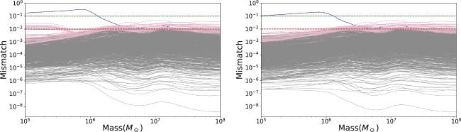
With regard to the high-frequency side, we check how the cutting frequency affects the waveform accuracy. For comparison, we have compared the results plotted in figure 4 to frequency choices
$\begin{eqnarray}{f}_{\mathrm{low}}=\max ({10}^{-5},{f}_{\min }),\end{eqnarray}$
$\begin{eqnarray}{f}_{\mathrm{up}}=\min (1,0.8{f}_{\max }),\end{eqnarray}$
and $\begin{eqnarray}{f}_{\mathrm{low}}=\max ({10}^{-5},{f}_{\min }),\end{eqnarray}$
$\begin{eqnarray}{f}_{\mathrm{up}}=\min (1,0.5{f}_{\max }).\end{eqnarray}$
The results are shown in figure 7. As expected, the high-frequency side affects large black hole mass systems more. But overall, the influence is small.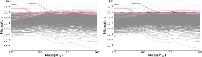
Furthermore, we have also considered a conservative frequency range choice on both the low- and high-frequency side
$\begin{eqnarray}{f}_{\mathrm{low}}=\max ({10}^{-5},1.5{f}_{\min }),\end{eqnarray}$
$\begin{eqnarray}{f}_{\mathrm{up}}=\min (1,0.8{f}_{\max }).\end{eqnarray}$
The results are plotted in figure 8. In summary, the different frequency choices roughly result in similar waveform accuracy.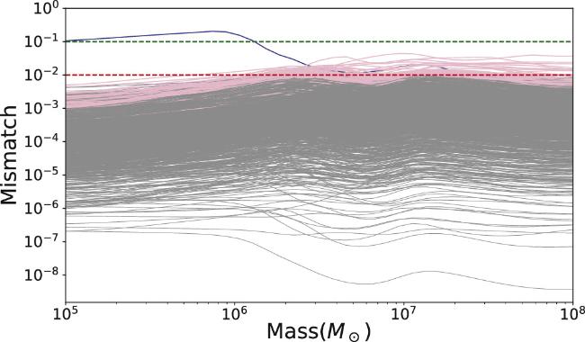
4. Summary and conclusion
One of the most challenging and fascinating problems in gravitational physics is to understand the dynamics of binary black hole mergers in the strong-field regime. In this regime, the components of the binary move at relativistic speeds and the spacetime curvature becomes highly nonlinear, making analytical approximations inadequate. The only reliable way to obtain precise solutions to Einstein's field equations in this regime is to use numerical relativity, which involves solving the full nonlinear equations on high-performance computers. This breakthrough was achieved in 2005 after decades of efforts [22].
Numerical relativity simulations of binary black hole mergers are essential for modeling the gravitational wave signals emitted by these systems during their late inspiral, merger and ringdown phases. These signals are used to infer the properties of the source systems and to test general relativity in extreme conditions. All binary black hole detections made by LIGO and Virgo have been analyzed using waveform models that incorporate numerical relativity data. The most prominent examples of these models are the effective-one-body and phenomenological waveform models. Numerical relativity also plays a key role in validating these models and testing their accuracy and robustness. Moreover, numerical relativity waveforms can be directly used for parameter estimation, template bank construction and waveform family development without intermediate analytical steps, using techniques such as reduced-order modeling.
Several coordinated efforts have been undertaken to produce numerical relativity simulations of binary black hole mergers for gravitational wave applications. These include the Numerical Injection Analysis (NINJA) project [51], the collaboration between Numerical Relativity and Analytical Relativity (NRAR) and the waveform catalogs released by the SXS collaboration and Georgia Tech.
In this work, we use numerical simulations of binary black hole mergers performed by the SXS collaboration using the Spectral Einstein Code (SpEC). The SXS catalog has been used to construct the SEOBNRE waveform model [28–31] and other waveform models. The accuracy of the numerical relativity waveform is very important to gravitational wave astronomy study.
In previous works, the accuracy issue of numerical relativity waveforms has been well studied for ground-based detectors. In the current paper, we focus on space-based detectors. We have systematically investigated the effects of the waveform frequency range, the detector sensitivity detail, the BBH's black hole mass and others on the waveform accuracy issue.
Each waveform of the SXS catalog has been investigated. Special attention is paid to matching factor calculation between the highest and second-highest resolution used in the numerical simulations. Our calculation results indicate that the numerical relativity waveforms are as accurate as 99% with respect to space-based detectors, including LISA, Taiji and Tianqin. Such an accuracy level is comparable to that with respect to LIGO. If only the accuracy requirement for space-based detectors is similar to that of ground-based ones, the current numerical relativity waveforms are valid for waveform modelling.