


1. Introduction
Lump solutions are special analytical rational function solutions in soliton theory, which were first found in the study of the Kadomtsev–Petviashvili (KP) equation [1]. Lump solutions have been widely applied in the fields of Bose–Einstein condensation, ocean waves, optics, shallow water waves and so on [2–8], and have been paid increasing attention by mathematicians in recent years [9–14]. Therefore, it is of great significance to study lump solutions of nonlinear differential equations. To get lump solutions of nonlinear differential equations, many methods have been proposed, such as Darboux transformation [15], the long-wave limit method [16, 17], Hirota’s bilinear method [18], the trigonometric function series method [19] and the Jacobi elliptic function expansion method [20]. The long-wave limit method was first proposed by Ablowitz et al [16, 17]. However, by taking the long-wave limit, one can only get lump solutions which are localized in the all-plane of the nonlinear differential equations less than (2+1)-dimensional, while the lump solutions localized in the all-plane of the (3+1)-dimensional nonlinear differential equations cannot be guaranteed.
It is always a hot topic to seek the exact solutions, such as breath-wave solutions [21, 22], interaction solutions [23] and lump solutions [24–26], of nonlinear differential equations, and many exact solutions of nonlinear differential equations have been obtained by some scholars in recent years. For instance, Chen et al derived the breather solutions and the interaction solutions of the (3+1)-dimensional generalized Camassa–Holm KP equation [27]. The mixed lump-stripe solutions and the mixed rogue wave-stripe solutions of the (3+1)-dimensional nonlinear wave equation were obtained by Wang et al [28]. Li and Jiang obtained the lump solutions of the (2+1)-dimensional Hietarina-like equation [29]. Based on the long-wave limit method, Liu obtained the lump solutions of the (2+1)-dimensional generalized Calogero–Bogoyavlenshii–Schiff (CBS) equation [30], while Cao et al obtained the lump solutions to the potential KP equation and (2+1)-dimensional Sawada–Kotera equation using the same method, respectively [31, 32]. With the aid of Hirota’s bilinear method, Pu et al obtained the lump solutions of the (3+1)-dimensional soliton equation and the expanded Jimbo–Miwa equation [33, 34]. In [35], Ma first proposed a quadratic function method for constructing lump solutions of nonlinear differential equations, which can gain the lump solutions of high-dimensional nonlinear differential equations localized in the whole plane. Subsequently, Zhou et al derived the lump solutions of the (3+1)-dimensional generalized CBS equation and reduced the (3+1)-dimensional nonlinear evolution equation using a quadratic function method [36, 37]. Inspired by the study of Ma et al, this paper aims to derive the lump solutions localized in the whole plane of a more generalized (3+1)-dimensional nonlinear differential equation1 ) can be transformed into the following Hirota’s bilinear form1 ) can be reduced to many classical integrable equations. Here, we present the following examples.
$\begin{eqnarray}\begin{array}{l}{{au}}_{t}+b\left({u}_{{xxz}}+3{{uu}}_{z}+3{u}_{x}{\partial }^{-1}{u}_{z}\right)+c\left({u}_{{xxy}}+3{{uu}}_{y}\right.\\ \quad \left.+3{u}_{x}{\partial }^{-1}{u}_{y}\right)+{{du}}_{x}+{{gu}}_{y}+{{hu}}_{z}=0,\end{array}\end{eqnarray}$
where $\begin{eqnarray*}{\partial }^{-1}{u}_{z}=\int {u}_{z}{\rm{d}}x,{\partial }^{-1}{u}_{y}=\int {u}_{y}{\rm{d}}x,\end{eqnarray*}$
and a, b, c, d, g and h are any nonzero constants. Through the transformation $\begin{eqnarray}u=2{\left(\mathrm{ln}f\right)}_{{xx}},\end{eqnarray}$
equation ( $\begin{eqnarray}\begin{array}{l}\left({{aD}}_{x}{D}_{t}+{{bD}}_{x}^{3}{D}_{z}+{{cD}}_{x}^{3}{D}_{y}+{{dD}}_{x}^{2}\right.\\ \quad \left.+{{gD}}_{x}{D}_{y}+{{hD}}_{x}{D}_{z}\right)f\cdot f=0.\end{array}\end{eqnarray}$
When different parameters are selected for the coefficients a, b, c, d, g and h, equation (When a = b = 1, c = d = g = h = 0 and z = x, equation (1 ) is reduced to the Korteweg–de Vries (KdV) equation1 ) is reduced to the (2+1)-dimensional generalized Konopelchenko–Dubrovsky–Kaup–Kupershmidt equation [38]1 ) is reduced to the (2+1)-dimensional generalized Bogoyavlensky–Konopelchenko (BK) equation [39]1 ) can be widely used in ocean dynamics and other related fields, and the study of equation (1 ) is helpful for us to find the lump solutions of KdV-type equations. In the following, the lump solutions localized in the full plane are shortened to lump solutions.
$\begin{eqnarray*}{u}_{t}+{u}_{{xxx}}+6{{uu}}_{x}=0.\end{eqnarray*}$
When a = 1, b = h1, c = h5, g = 0, d + h = 0 and z = x, equation ( $\begin{eqnarray*}\begin{array}{l}{u}_{t}+{h}_{1}{u}_{{xxx}}+{h}_{2}{{uu}}_{x}+{h}_{3}{u}_{{xxxxx}}+{h}_{4}{v}_{y}+{h}_{5}{u}_{{xxy}}\\ +{h}_{6}\left({u}_{x}v+{{uv}}_{x}\right)+{h}_{7}\left({u}_{x}{u}_{{xx}}+{{uu}}_{{xxx}}\right)+{h}_{8}{u}^{2}{u}_{x}=0,\end{array}\end{eqnarray*}$
$\begin{eqnarray*}{v}_{x}={u}_{y}\end{eqnarray*}$
for h2 = 6h1, h6 = 3h5, h3 = h4 = h7 = h8 = 0, where ${h}_{i}\left(i=1,2,\ldots ,8\right)$ is an arbitrary real constant. When a = 1, b = α, c = β, d = γ1, g = γ2, h = 0 and z = x, equation ( $\begin{eqnarray}\begin{array}{l}{u}_{t}+\alpha \left(6{{uu}}_{x}+{u}_{{xxx}}\right)+\beta \left({u}_{{xxy}}+3{{uu}}_{y}+3{u}_{x}{v}_{y}\right)\\ \quad +{\gamma }_{1}{u}_{x}+{\gamma }_{2}{u}_{y}+{\gamma }_{3}{v}_{{yy}}=0,\\ \quad {v}_{x}=u\end{array}\end{eqnarray}$
for γ3 = 0, where α, β, γ1, γ2 and γ3 are constants. Equation (The structure of this paper is organized as follows. In section 2 , a lump solution is obtained using the quadratic function method. In section 3 , we briefly introduce the amplitude of the lump wave and its propagation velocities along the x, y and z axes, respectively, and a theorem describing the amplitude and propagation velocity of this lump wave is established. In section 4 , we show 3D plots and the corresponding density plots of the lump waves from three examples. In section 5 , we obtain the breath-wave solutions of equation (1 ). In section 6 , several interaction solutions of equation (1 ) are studied. Finally, some conclusions are given in the last section.
2. Lump solutions in (3+1)-dimensional of equation (1 )
In this section, we introduce the method of finding the lump solutions. Based on the study of [35], we know that the positive quadratic function solution of equation (1 ) can be expressed as5 ) to get a lump solution in (3+1)-dimensional. Therefore, we use the following method to find the lump solution. A useful lemma is introduced as follows.
$\begin{eqnarray}f={f}_{1}^{2}+{f}_{2}^{2}+{f}_{3}^{2}+q,\end{eqnarray}$
where fj = d1jx + d2jy + d3jz + d4jt + d5j with d1j, d2j, d3j, d4j and ${d}_{5j}\left(j=1,2,3\right)$ being constants. It is difficult to obtain the sum of three squares of f by equation (Let $\beta ={\left({\beta }_{1},\cdots ,{\beta }_{N}\right)}^{T}\in {{\mathbb{R}}}^{N}$ be a fixed vector and consider the following quadratic function
$\begin{eqnarray}\begin{array}{l}f\left(x\right)={\left(x-\beta \right)}^{T}B\left(x-\beta \right)+q\\ \quad =\displaystyle \sum _{i,j=1}^{N}{b}_{{ij}}\left({x}_{i}-{\beta }_{i}\right)\left({x}_{j}-{\beta }_{j}\right)+q,\end{array}\end{eqnarray}$
where the real matrix $B={\left({b}_{{ij}}\right)}_{N\times N}$ is symmetric and $q\in {\mathbb{R}}$ is a constant. The function f defined by equation ( $\begin{eqnarray*}P\left(D\right)f\cdot f=P\left({D}_{1},{D}_{2},\cdots {D}_{N}\right)f\cdot f=0\end{eqnarray*}$
if and only if $\begin{eqnarray*}2\displaystyle \sum _{i,j,k,l=1}^{N}{p}_{{ijkl}}\left({b}_{{ij}}{b}_{{kl}}+{b}_{{ik}}{b}_{{jl}}+{b}_{{il}}{b}_{{jk}}\right)+q\displaystyle \sum _{i,j=1}^{N}{p}_{{ij}}{b}_{{ij}}=0\end{eqnarray*}$
and $\begin{eqnarray*}\displaystyle \sum _{i,j=1}^{N}{p}_{{ij}}\left({b}_{{ij}}B-{B}_{i}{B}_{j}^{T}-{B}_{j}{B}_{i}^{T}\right)=0,\end{eqnarray*}$
where P is a polynomial of N variables and $D\,=\left({D}_{1},{D}_{2},\cdots {D}_{N}\right),$ ${B}_{i}$ denotes the ith column vector of the symmetric matrix B for $1\leqslant i\leqslant N,$ ${p}_{{ij}}$ and ${p}_{{ijkl}}$ are the coefficients of the quadratic and quartic terms, respectively [35].Let7 ) is a solution to equation (1 ) if and only if3 ) contains the second-order Hirota derivative terms, theorem 3.6 in [35] shows that equation (3 ) has a positive quadratic function solution when $\left|B\right|=0.$ Thus, to satisfy $\left|B\right|=0,$ we set ${Rank}\left(B\right)=3$, then we get m = 0. Substituting m = 0 into equation (10 ), we obtain that $q\left(q\gt 0\right)$ is an arbitrary constant and ${b}_{1}\left({{bb}}_{3}+{{cb}}_{2}\right)=0$. Since B is a semi-positive definite matrix, all the principal entries of B are non-negative. If b1 = 0, then1 ) has no lump solution. Therefore, we have to set bb3 + cb2 = 0, namely ${b}_{3}=-\tfrac{c}{b}{b}_{2}$. Then, the non-trivial solutions of equation (11 ) can be written as
$\begin{eqnarray}f={\alpha }^{T}B\alpha +q,\end{eqnarray}$
where $\alpha ={\left(x,y,z,t\right)}^{T},B=\left[{b}_{{ij}}\right]$ is a 4 × 4 symmetric matrix, and q is a constant. We introduce two matrices $\begin{eqnarray}P=\left(\begin{array}{cccc}2d & g & h & a\\ g & 0 & 0 & 0\\ h & 0 & 0 & 0\\ a & 0 & 0 & 0\end{array}\right),\,\,\,\,\,\,\,\,B=\left(\begin{array}{cccc}{b}_{1} & {b}_{2} & {b}_{3} & {b}_{4}\\ {b}_{2} & {b}_{5} & {b}_{6} & {b}_{7}\\ {b}_{3} & {b}_{6} & {b}_{8} & {b}_{9}\\ {b}_{4} & {b}_{7} & {b}_{9} & {b}_{10}\end{array}\right),\end{eqnarray}$
then define $\begin{eqnarray}m=\displaystyle \frac{1}{2}\displaystyle \sum _{i,j=1}^{4}P\left(i,j\right)B\left(i,j\right)={{db}}_{1}+{{gb}}_{2}+{{hb}}_{3}+{{ab}}_{4},\end{eqnarray}$
where $P\left(i,j\right)$ and $B\left(i,j\right)$ are used to represent the ith row and jth column elements of matrices P and B, respectively. From lemma 1, the function f defined by equation ( $\begin{eqnarray}6\left({{bb}}_{1}{b}_{3}+{{cb}}_{1}{b}_{2}\right)+{mq}=0,\end{eqnarray}$
$\begin{eqnarray}{mB}-{BPB}=0.\end{eqnarray}$
Since equation ( $\begin{eqnarray*}\left|\begin{array}{cc}{b}_{1} & {b}_{2}\\ {b}_{2} & {b}_{5}\end{array}\right|={b}_{1}{b}_{5}-{b}_{2}^{2}=-{b}_{2}^{2}\geqslant 0,\end{eqnarray*}$
hence b2 = 0. Furthermore, we have b3 = b4 = 0. Then, we get a trivial solution to f that does not depend on x and, from theorem 2 in [36], equation ( $\begin{eqnarray}\begin{array}{l}{b}_{1}=\displaystyle \frac{a\left({{gb}}_{7}+{{hb}}_{9}+{{ab}}_{10}\right)}{{d}^{2}},\\ {b}_{2}={b}_{3}=0,{b}_{4}=-\displaystyle \frac{{{gb}}_{7}+{{hb}}_{9}+{{ab}}_{10}}{d},\\ {b}_{5}=\displaystyle \frac{{h}^{2}{b}_{8}+{{ahb}}_{9}-{{agb}}_{7}}{{g}^{2}},{b}_{6}=-\displaystyle \frac{{{hb}}_{8}+{{ab}}_{9}}{g},\end{array}\end{eqnarray}$
where a, d, g and h are any nonzero constants, while b7, b8, b9 and b10 are free variables such that B ≥ 0 and ${Rank}\left(B\right)=3$.Substituting equation (12 ) into B in equation (8 ), we get the matrix B5 ) can be expressed as
$\begin{eqnarray*}\left(\begin{array}{cccc}\displaystyle \frac{a\left({{gb}}_{7}+{{hb}}_{9}+{{ab}}_{10}\right)}{{d}^{2}} & 0 & 0 & -\displaystyle \frac{{{gb}}_{7}+{{hb}}_{9}+{{ab}}_{10}}{d}\\ 0 & \displaystyle \frac{{h}^{2}{b}_{8}+{{ahb}}_{9}-{{agb}}_{7}}{{g}^{2}} & -\displaystyle \frac{{{hb}}_{8}+{{ab}}_{9}}{g} & {b}_{7}\\ 0 & -\displaystyle \frac{{{hb}}_{8}+{{ab}}_{9}}{g} & {b}_{8} & {b}_{9}\\ -\displaystyle \frac{{{gb}}_{7}+{{hb}}_{9}+{{ab}}_{10}}{d} & {b}_{7} & {b}_{9} & {b}_{10}\end{array}\right)\end{eqnarray*}$
and the function f defined by equation ( $\begin{eqnarray*}\begin{array}{l}f\left(x,y,z,t\right)=\displaystyle \frac{a\left({{gb}}_{7}+{{hb}}_{9}+{{ab}}_{10}\right)}{{d}^{2}}{\left(x-\displaystyle \frac{d}{a}t\right)}^{2}\\ \quad +\displaystyle \frac{{h}^{2}{b}_{8}+{{ahb}}_{9}}{{g}^{2}}{\left(y-\displaystyle \frac{g}{h}z\right)}^{2}\end{array}\end{eqnarray*}$
$\begin{eqnarray}-\displaystyle \frac{{{ab}}_{7}}{g}{\left(y-\displaystyle \frac{g}{a}t\right)}^{2}-\displaystyle \frac{{{ab}}_{9}}{h}{\left(z-\displaystyle \frac{h}{a}t\right)}^{2}+q.\end{eqnarray}$
Taking the appropriate parameters, such that $\begin{eqnarray}\begin{array}{l}\displaystyle \frac{a\left({{gb}}_{7}+{{hb}}_{9}+{{ab}}_{10}\right)}{{d}^{2}}\gt 0,\displaystyle \frac{{h}^{2}{b}_{8}+{{ahb}}_{9}}{{g}^{2}}\gt 0,\\ \quad -\displaystyle \frac{{{ab}}_{7}}{g}\gt 0,-\displaystyle \frac{{{ab}}_{9}}{h}\gt 0,q\gt 0,\end{array}\end{eqnarray}$
then function f is positive definite.By symbolic computations, we obtain13 ). If the appropriate parameters are chosen so that16 ) holds, then function f depends on x, y, z and t, thus15 ) produces a lump solution of equation (1 ).
$\begin{eqnarray*}\begin{array}{l}f\left(x,y,z,t\right)=\displaystyle \frac{{\left({{hb}}_{8}+{{ab}}_{9}\right)}^{2}}{{g}^{2}{b}_{8}}\\ \quad \times {\left(y-\displaystyle \frac{{{gb}}_{8}}{{{hb}}_{8}+{{ab}}_{9}}z-\displaystyle \frac{{{gb}}_{9}}{{{hb}}_{8}+{{ab}}_{9}}t\right)}^{2}\end{array}\end{eqnarray*}$
$\begin{eqnarray}\begin{array}{l}+\displaystyle \frac{a\left({{gb}}_{7}+{{hb}}_{9}+{{ab}}_{10}\right)}{{d}^{2}}{\left(x-\displaystyle \frac{d}{a}t\right)}^{2}\\ \quad -\displaystyle \frac{a\left({{ab}}_{9}^{2}+{{hb}}_{8}{b}_{9}+{{gb}}_{7}{b}_{8}\right)}{{g}^{2}{b}_{8}}{\left(y-\displaystyle \frac{g}{a}t\right)}^{2}+q\end{array}\end{eqnarray}$
from equation ( $\begin{eqnarray}\begin{array}{l}\displaystyle \frac{{\left({{hb}}_{8}+{{ab}}_{9}\right)}^{2}}{{g}^{2}{b}_{8}}\gt 0,\displaystyle \frac{a\left({{gb}}_{7}+{{hb}}_{9}+{{ab}}_{10}\right)}{{d}^{2}}\gt 0,\\ \quad -\displaystyle \frac{a\left({{ab}}_{9}^{2}+{{hb}}_{8}{b}_{9}+{{gb}}_{7}{b}_{8}\right)}{{g}^{2}{b}_{8}}\gt 0,q\gt 0,\end{array}\end{eqnarray}$
then function f is positive definite. If equation ( $\begin{eqnarray*}D=\left|\begin{array}{ccc}{d}_{11} & {d}_{21} & {d}_{31}\\ {d}_{12} & {d}_{22} & {d}_{32}\\ {d}_{13} & {d}_{23} & {d}_{33}\end{array}\right|\ne 0.\end{eqnarray*}$
Therefore, according to theorem 2 in [36], the function f defined by equation (Lump solutions localized in the whole plane of any (3+1)-dimensional nonlinear evolution equation cannot be obtained by taking the long-wave limit of the two-soliton solutions, but can be obtained via the quadratic function method [36].
3. The amplitude and propagation velocity of the lump waves
In this section, we obtain the amplitude of the lump produced by equation (15 ) and its propagation velocities along the x, y and z axes. Substituting equation (15 ) into equation (2 ), a lump solution
$\begin{eqnarray*}\begin{array}{l}u=2{\left(\mathrm{ln}f\right)}_{{xx}}=4{g}^{2}\left({{gb}}_{7}+{{hb}}_{9}+{{ab}}_{10}\right)\\ \quad \times \left[-\left({a}^{2}{g}^{3}{b}_{7}+{a}^{3}{g}^{2}{b}_{10}+{a}^{2}{g}^{2}{{hb}}_{9}\right){x}^{2}\right.\end{array}\end{eqnarray*}$
$\begin{eqnarray*}\begin{array}{l}+\left({a}^{2}{d}^{2}{{hb}}_{9}-{a}^{2}{d}^{2}{{gb}}_{7}+{{ad}}^{2}{h}^{2}{b}_{8}\right){y}^{2}+{{ad}}^{2}{g}^{2}{b}_{8}{z}^{2}\\ \quad -\left(2{d}^{2}{g}^{3}{b}_{7}+2{d}^{2}{g}^{2}{{hb}}_{9}+{{ad}}^{2}{g}^{2}{b}_{10}\right){t}^{2}\end{array}\end{eqnarray*}$
$\begin{eqnarray*}\begin{array}{l}+2\left({{adg}}^{3}{b}_{7}+{a}^{2}{{dg}}^{2}{b}_{10}+{{adg}}^{2}{{hb}}_{9}\right){xt}\\ \quad +2{{ad}}^{2}{g}^{2}{b}_{7}{yt}+2{{ad}}^{2}{g}^{2}{b}_{9}{zt}\end{array}\end{eqnarray*}$
$\begin{eqnarray*}\begin{array}{l}-2\left({a}^{2}{d}^{2}{{gb}}_{9}+{{ad}}^{2}{{ghb}}_{8}\right){yz}\left.+{{ad}}^{2}{g}^{2}q\right]/\\ \left[\left({{ag}}^{2}{{hb}}_{9}+{{ag}}^{3}{b}_{7}+{a}^{2}{g}^{2}{b}_{10}\right){x}^{2}\right.\end{array}\end{eqnarray*}$
$\begin{eqnarray*}\begin{array}{l}+\left({{ad}}^{2}{{hb}}_{9}+{d}^{2}{h}^{2}{b}_{8}-{{ad}}^{2}{{gb}}_{7}\right){y}^{2}+{d}^{2}{g}^{2}{b}_{8}{z}^{2}+{d}^{2}{g}^{2}{b}_{10}{t}^{2}\\ \quad -2\left({{dg}}^{2}{{hb}}_{9}+{{dg}}^{3}{b}_{7}+{{adg}}^{2}{b}_{10}\right){xt}\end{array}\end{eqnarray*}$
$\begin{eqnarray}\begin{array}{l}+2{d}^{2}{g}^{2}{b}_{7}{yt}+2{d}^{2}{g}^{2}{b}_{9}{zt}-2\\ \quad \left({d}^{2}{{ghb}}_{8}+{{ad}}^{2}{{gb}}_{9}\right){yz}{\left.+{d}^{2}{g}^{2}q\right]}^{2}\end{array}\end{eqnarray}$
is obtained.Taking partial derivatives of x, y and z, respectively, in equation (15 ), we have17 ), along the x, y and z axes. Substituting $x=\tfrac{d}{a}t,y=\tfrac{g}{a}t$ and $z=\tfrac{h}{a}t$ into equation (17 ), we get the amplitude of the lump, equation (17 )
$\begin{eqnarray*}\begin{array}{l}{f}_{x}=\displaystyle \frac{2a\left({{gb}}_{7}+{{hb}}_{9}+{{ab}}_{10}\right)}{{d}^{2}}\left(x-\displaystyle \frac{d}{a}t\right),\\ {f}_{y}=\displaystyle \frac{2\left({h}^{2}{b}_{8}^{2}+{{ahb}}_{8}{b}_{9}-{{agb}}_{7}{b}_{8}\right)}{{g}^{2}{b}_{8}}y\\ -\displaystyle \frac{2\left({{hb}}_{8}+{{ab}}_{9}\right)}{g}z+2{b}_{7}t,\\ {f}_{z}=-\displaystyle \frac{2\left({{hb}}_{8}+{{ab}}_{9}\right)}{g}y+2{b}_{8}z+2{b}_{9}t.\end{array}\end{eqnarray*}$
Let $\begin{eqnarray*}{f}_{x}={f}_{y}={f}_{z}=0,\end{eqnarray*}$
and we obtain $\begin{eqnarray*}x=\displaystyle \frac{d}{a}t,\,\,y=\displaystyle \frac{g}{a}t,\,\,z=\displaystyle \frac{h}{a}t,\end{eqnarray*}$
where the coefficients $\tfrac{d}{a},\tfrac{g}{a}$ and $\tfrac{h}{a}$ of t are, respectively, the propagation velocities of the lump, equation ( $\begin{eqnarray}H=\displaystyle \frac{4a\left({{gb}}_{7}+{{hb}}_{9}+{{ab}}_{10}\right)}{{{qd}}^{2}}.\end{eqnarray}$
Based on the above discussion, we give the following theorem.For a bilinear equation of the form
$\begin{eqnarray*}\begin{array}{l}\left({{aD}}_{x}{D}_{t}+{{bD}}_{x}^{3}{D}_{z}+{{cD}}_{x}^{3}{D}_{y}+{{dD}}_{x}^{2}\right.\\ \quad \left.+{{gD}}_{x}{D}_{y}+{{hD}}_{x}{D}_{z}\right)f\cdot f=0,\end{array}\end{eqnarray*}$
it has a lump solution with amplitude $\begin{eqnarray*}H=\displaystyle \frac{4a\left({{gb}}_{7}+{{hb}}_{9}+{{ab}}_{10}\right)}{{{qd}}^{2}}\end{eqnarray*}$
and the propagation velocities along the $x,y,$ and z axes are $\tfrac{d}{a},\tfrac{g}{a}$ and $\tfrac{h}{a}$, respectively.4. Three examples
In this section, we will give three examples of the lump solutions to equations like equation (1 ) based on theorem 1.
Case 1. We take a = b = c = d = g = 1, h = − 1, b7 = − 2, b8 = 6, b9 = 1, b10 = 10 and q = 1. Then the matrix15 ), we know19 ) for (a) x = 0, (b) y = 0, (c) z = 0 when t = 0, and the corresponding density plots of equation (19 ) for (d) x = 0, (e) y = 0, (f) z = 0 when t = 0.
$\begin{eqnarray*}B=\left(\begin{array}{cccc}7 & 0 & 0 & -7\\ 0 & 3 & 5 & -2\\ 0 & 5 & 6 & 1\\ -7 & -2 & 1 & 10\end{array}\right)\end{eqnarray*}$
is positive semi-definite. By considering equation ( $\begin{eqnarray*}f=\displaystyle \frac{25}{6}{\left(y+\displaystyle \frac{6}{5}z+\displaystyle \frac{1}{5}t\right)}^{2}+7{\left(x-t\right)}^{2}+\displaystyle \frac{17}{6}{\left(y-t\right)}^{2}+1.\end{eqnarray*}$
Then the function $\begin{eqnarray}\begin{array}{l}u=2{\left(\mathrm{ln}f\right)}_{{xx}}=\displaystyle \frac{28\left(7{y}^{2}+10{yz}-4{yt}+6{z}^{2}+2{zt}-4{t}^{2}-7{x}^{2}+14{xt}+1\right)}{{\left(7{y}^{2}+10{yz}-4{yt}+6{z}^{2}+2{zt}+10{t}^{2}+7{x}^{2}-14{xt}+1\right)}^{2}}\end{array}\end{eqnarray}$
is a lump solution to the equation $\begin{eqnarray*}\left({D}_{x}{D}_{t}+{D}_{x}^{3}{D}_{z}+{D}_{x}^{3}{D}_{y}+{D}_{x}^{2}+{D}_{x}{D}_{y}-{D}_{x}{D}_{z}\right)f\cdot f=0.\end{eqnarray*}$
This lump has an amplitude of 28, and the propagation velocities of this lump along the x, y, z axes are 1, 1, − 1, respectively, where the negative sign is the direction of propagation of the lump wave. Figure 1 shows the 3D plots of equation (
Figure 1. The 3D plots of equation ( |
Case 2. We take a = − 1, b = c = 2, d = 1, g = h = − 2, b7 = − 1, b8 = 5, b9 = − 2, b10 = 12 and q = 2. Then the matrix15 ), we have20 ) for (a) x = 0, (b) y = 0, (c) z = 0 when t = 0, and the corresponding density plots of equation (20 ) for (d) x = 0, (e) y = 0, (f) z = 0 when t = 0.
$\begin{eqnarray*}B=\left(\begin{array}{cccc}6 & 0 & 0 & 6\\ 0 & \displaystyle \frac{9}{2} & -4 & -1\\ 0 & -4 & 5 & -2\\ 6 & -1 & -2 & 12\end{array}\right)\end{eqnarray*}$
is positive semi-definite. By considering equation ( $\begin{eqnarray*}f=\displaystyle \frac{16}{5}{\left(y-\displaystyle \frac{5}{4}z+\displaystyle \frac{1}{2}t\right)}^{2}+6{\left(x+t\right)}^{2}+\displaystyle \frac{13}{10}{\left(y-2t\right)}^{2}+2.\end{eqnarray*}$
Then the function $\begin{eqnarray}\begin{array}{l}u=2{\left(\mathrm{ln}f\right)}_{{xx}}=\displaystyle \frac{48\left(9{y}^{2}-16{yz}-4{yt}+10{z}^{2}-8{zt}-12{x}^{2}-24{xt}+4\right)}{{\left(9{y}^{2}-16{yz}-4{yt}+10{z}^{2}-8{zt}+24{t}^{2}+12{x}^{2}+24{xt}+4\right)}^{2}}\end{array}\end{eqnarray}$
is a lump solution to the equation $\begin{eqnarray*}\begin{array}{l}\left(-{D}_{x}{D}_{t}+2{D}_{x}^{3}{D}_{z}+2{D}_{x}^{3}{D}_{y}\right.\\ \quad \left.+{D}_{x}^{2}-2{D}_{x}{D}_{y}-2{D}_{x}{D}_{z}\right)f\cdot f=0.\end{array}\end{eqnarray*}$
The amplitude of this lump is 12, and the propagation velocities of this lump along the x, y, z axes are −1, 2, 2, respectively. Figure 2 shows the 3D plots of equation (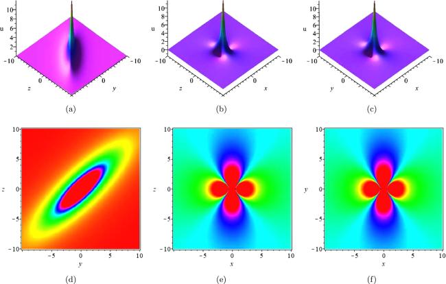
Figure 2. The 3D plots of equation ( |
Case 3. We take a = b = d = 2, c = 1, g = − 3, h = 0, b7 = 1, b8 = 8, b9 = 1, b10 = 15, q = 3, and z = x. Then the matrix15 ), we have4 ) for γ3 = 0. The amplitude of this lump is 18, and the propagation velocities of this lump along the x and y axes are 1 and $-\tfrac{3}{2},$ respectively. Figure 3 shows the 3D plots and corresponding density plots of the projection of the lump solution, equation (21 ), when t = 0, t = 5 and t = 10.
$\begin{eqnarray*}B=\left(\begin{array}{cccc}\displaystyle \frac{27}{2} & 0 & 0 & -\displaystyle \frac{27}{2}\\ 0 & \displaystyle \frac{2}{3} & \displaystyle \frac{2}{3} & 1\\ 0 & \displaystyle \frac{2}{3} & 8 & 1\\ -\displaystyle \frac{27}{2} & 1 & 1 & 15\end{array}\right)\end{eqnarray*}$
is positive semi-definite. By considering equation ( $\begin{eqnarray*}\begin{array}{l}f=\displaystyle \frac{1}{18}{\left(y+12x+\displaystyle \frac{3}{2}t\right)}^{2}+\displaystyle \frac{27}{2}{\left(x-t\right)}^{2}\\ \quad +\displaystyle \frac{11}{18}{\left(y+\displaystyle \frac{3}{2}t\right)}^{2}+3.\end{array}\end{eqnarray*}$
Then the function $\begin{eqnarray}\begin{array}{l}u=2{\left(\mathrm{ln}f\right)}_{{xx}}=\displaystyle \frac{4\left(484{y}^{2}-1032{xy}+2748{yt}-16\,641{x}^{2}+19\,350{xt}+360{t}^{2}+2322\right)}{{\left(4{y}^{2}+8{xy}+12{yt}+129{x}^{2}-150{xt}+90{t}^{2}+18\right)}^{2}}\end{array}\end{eqnarray}$
is a lump solution to the equation $\begin{eqnarray*}\left(2{D}_{x}{D}_{t}+2{D}_{x}^{4}+{D}_{x}^{3}{D}_{y}+2{D}_{x}^{2}-3{D}_{x}{D}_{y}\right)f\cdot f=0,\end{eqnarray*}$
which is a bilinear equation of the (2+1)-dimensional generalized BK equation (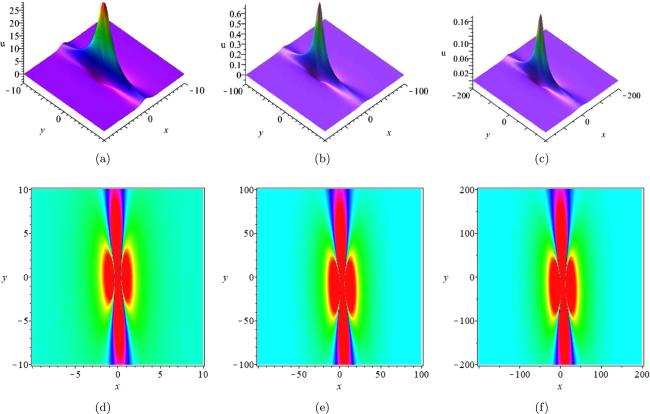
Figure 3. The 3D plots of equation ( |
5. The breath-wave solutions of equation (1 )
In this section, we focus on finding the breath-wave solutions of equation (1 ). We set22 ) into bilinear equation (3 ), we get23 ) into equation (22 ) yields2 ), we get24 ) under different parameters. As seen in figure 4(b), when the ϵ5 decreases to $-\tfrac{2}{5}$ and the ϵ7 increases to 2, the breath waves become denser than those in figure 4(a). In figure 4(c), we find that when the parameter ϵ1 is reduced to $\tfrac{1}{5}$, the twist angle of the breath waves are changed.
$\begin{eqnarray}f={{\rm{e}}}^{-{\mu }_{1}{\phi }_{1}}+{\delta }_{1}\cos \left({\mu }_{2}{\phi }_{2}\right)+{\delta }_{2}{{\rm{e}}}^{{\mu }_{1}{\phi }_{1}},\end{eqnarray}$
where μ1, μ2, δ1 and δ2 are nonzero constants and $\begin{eqnarray*}\begin{array}{l}{\phi }_{1}={\varepsilon }_{1}x+{\varepsilon }_{2}y+{\varepsilon }_{3}z+{\varepsilon }_{4}t+{\varepsilon }_{5},\\ {\phi }_{2}={\varepsilon }_{6}x+{\varepsilon }_{7}y+{\varepsilon }_{8}z+{\varepsilon }_{9}t+{\varepsilon }_{10}\end{array}\end{eqnarray*}$
with ${\varepsilon }_{i}\left(i=1,\ldots ,10\right)$ being an undetermined constant. Substituting equation ( $\begin{eqnarray}\begin{array}{l}{\delta }_{2}=-\displaystyle \frac{{\delta }_{1}^{2}\left(3{\varepsilon }_{6}^{2}{\mu }_{2}^{2}+{\varepsilon }_{1}^{2}{\mu }_{1}^{2}\right)}{8{\varepsilon }_{1}^{2}{\mu }_{1}^{2}},\,\,\,\,\,\,\,\,\,\,\,\,{\varepsilon }_{2}=-\displaystyle \frac{b{\varepsilon }_{3}}{c},\\ {\varepsilon }_{4}=\displaystyle \frac{{bg}{\varepsilon }_{3}+2c{\varepsilon }_{1}{\varepsilon }_{6}{\mu }_{2}^{2}\left(c{\varepsilon }_{7}+b{\varepsilon }_{8}\right)-c\left(d{\varepsilon }_{1}+h{\varepsilon }_{3}\right)}{{ac}},\\ {\varepsilon }_{9}=\displaystyle \frac{\left({\varepsilon }_{6}^{2}{\mu }_{2}^{2}-{\varepsilon }_{1}^{2}{\mu }_{1}^{2}\right)\left(c{\varepsilon }_{7}+b{\varepsilon }_{8}\right)-d{\varepsilon }_{6}-g{\varepsilon }_{7}-h{\varepsilon }_{8}}{a},\end{array}\end{eqnarray}$
where a, b, c, d, g, h, ϵ1, ϵ3, ϵ5, ϵ6, ϵ7, ϵ8, ϵ10, μ1, μ2 and δ1 are arbitrary nonzero constants. Substituting equation ( $\begin{eqnarray*}\begin{array}{l}f={{\rm{e}}}^{-{\mu }_{1}\left[{\varepsilon }_{1}x-\displaystyle \frac{b{\varepsilon }_{3}}{c}y+{\varepsilon }_{3}z+\displaystyle \frac{{bg}{\varepsilon }_{3}+2c{\varepsilon }_{1}{\varepsilon }_{6}{\mu }_{2}^{2}\left(c{\varepsilon }_{7}+b{\varepsilon }_{8}\right)-c\left(d{\varepsilon }_{1}+h{\varepsilon }_{3}\right)}{{ac}}t+{\varepsilon }_{5}\right]}-\displaystyle \frac{{\delta }_{1}^{2}\left(3{\varepsilon }_{6}^{2}{\mu }_{2}^{2}+{\varepsilon }_{1}^{2}{\mu }_{1}^{2}\right)}{8{\varepsilon }_{1}^{2}{\mu }_{1}^{2}}{{\rm{e}}}^{{\mu }_{1}\left({\varepsilon }_{1}x+{\varepsilon }_{2}y+{\varepsilon }_{3}z+{\varepsilon }_{4}t+{\varepsilon }_{5}\right)}+{\delta }_{1}\cos \\ \cdot \left\{{\mu }_{2}\left[{\varepsilon }_{6}x+{\varepsilon }_{7}y+{\varepsilon }_{8}z+\displaystyle \frac{\left({\varepsilon }_{6}^{2}{\mu }_{2}^{2}-{\varepsilon }_{1}^{2}{\mu }_{1}^{2}\right)\left(c{\varepsilon }_{7}+b{\varepsilon }_{8}\right)-d{\varepsilon }_{6}-g{\varepsilon }_{7}-h{\varepsilon }_{8}}{a}t+{\varepsilon }_{10}\right]\right\},\end{array}\end{eqnarray*}$
and then, via the transformation, equation ( $\begin{eqnarray}\begin{array}{l}u=\displaystyle \frac{2\left[{\varepsilon }_{1}^{2}{\mu }_{1}^{2}{{\rm{e}}}^{-{\lambda }_{1}}-{\delta }_{1}{\varepsilon }_{1}^{2}{\mu }_{1}^{2}\cos \left({\mu }_{2}{\lambda }_{2}\right)-\tfrac{{\delta }_{1}^{2}{\lambda }_{3}{{\rm{e}}}^{{\lambda }_{1}}}{8}\right]}{{{\rm{e}}}^{-{\lambda }_{1}}+{\delta }_{1}\cos \left({\mu }_{2}{\lambda }_{2}\right)-\tfrac{{\delta }_{1}^{2}{\lambda }_{3}{{\rm{e}}}^{{\lambda }_{1}}}{8{\varepsilon }_{1}^{2}{\mu }_{1}^{2}}}\\ \quad -\displaystyle \frac{2\left[-{\varepsilon }_{1}{\mu }_{1}{{\rm{e}}}^{-{\lambda }_{1}}-{\delta }_{1}\sin \left({\mu }_{2}{\lambda }_{2}\right)-\tfrac{{\delta }_{1}^{2}{\lambda }_{3}{{\rm{e}}}^{{\lambda }_{1}}}{8{\varepsilon }_{1}{\mu }_{1}}\right]}{{\left[{{\rm{e}}}^{-{\lambda }_{1}}+{\delta }_{1}\cos \left({\mu }_{2}{\lambda }_{2}\right)-\tfrac{{\delta }_{1}^{2}{\lambda }_{3}{{\rm{e}}}^{{\lambda }_{1}}}{8{\varepsilon }_{1}^{2}{\mu }_{1}^{2}}\right]}^{2}},\end{array}\end{eqnarray}$
where $\begin{eqnarray*}\begin{array}{l}{\lambda }_{1}={\mu }_{1}\left[{\varepsilon }_{1}x-\displaystyle \frac{b{\varepsilon }_{3}}{c}y+{\varepsilon }_{3}z\right.\\ \quad \left.+\displaystyle \frac{{bg}{\varepsilon }_{3}+2c{\varepsilon }_{1}{\varepsilon }_{6}{\mu }_{2}^{2}\left(c{\varepsilon }_{7}+b{\varepsilon }_{8}\right)-c\left(d{\varepsilon }_{1}+h{\varepsilon }_{3}\right)}{{ac}}t+{\varepsilon }_{5}\right],\\ {\lambda }_{2}={\varepsilon }_{6}x+{\varepsilon }_{7}y+{\varepsilon }_{8}z\\ \quad +\displaystyle \frac{\left({\varepsilon }_{6}^{2}{\mu }_{2}^{2}-{\varepsilon }_{1}^{2}{\mu }_{1}^{2}\right)\left(c{\varepsilon }_{7}+b{\varepsilon }_{8}\right)-d{\varepsilon }_{6}-g{\varepsilon }_{7}-h{\varepsilon }_{8}}{a}t+{\varepsilon }_{10},\\ {\lambda }_{3}=3{\varepsilon }_{6}^{2}{\mu }_{2}^{2}+{\varepsilon }_{1}^{2}{\mu }_{1}^{2}.\end{array}\end{eqnarray*}$
We take a = b = c = d = g = h = 1. Figure 4 shows the density plots of equation (
Figure 4. Density plots of equation ( |
6. The interaction solutions of equation (1 )
In this section, we derive several interaction solutions of equation (1 ) and show corresponding plots to observe the structures of these solutions.
6.1. The mixed lump–soliton solutions of equation (1 )
Let25 ) into equation (3 ), we obtain26 ) into equation (25 ) generates2 ), we have28 ). Let z = 0, and take the derivative of equation (27 ) with respect to x and y; then it can be concluded from fx = fy = 0 that the central point coordinate of the lump is27 ). Thus, the distance between the lump and the soliton is
$\begin{eqnarray}f={s}_{1}^{2}+{s}_{2}^{2}+{s}_{3}+{r}_{16},\end{eqnarray}$
where $\begin{eqnarray*}\begin{array}{l}{s}_{1}={r}_{1}x+{r}_{2}y+{r}_{3}z+{r}_{4}t+{r}_{5},\\ {s}_{2}={r}_{6}x+{r}_{7}y+{r}_{8}z+{r}_{9}t+{r}_{10},\\ {s}_{3}={r}_{11}{{\rm{e}}}^{{r}_{12}x+{r}_{13}y+{r}_{14}z+{r}_{15}t}\end{array}\end{eqnarray*}$
and ${r}_{i}\left(i=1,\ldots ,16\right)$ is an undetermined constant. By substituting equation ( $\begin{eqnarray}\begin{array}{l}{r}_{3}=-\displaystyle \frac{{{cr}}_{2}}{b},\\ {r}_{4}=\displaystyle \frac{{{chr}}_{2}-{{bdr}}_{1}-{{bgr}}_{2}}{{ab}},\\ {r}_{7}=-\displaystyle \frac{{{br}}_{8}}{c},\\ {r}_{9}=\displaystyle \frac{{{bgr}}_{8}-{{chr}}_{8}-{{cdr}}_{6}}{{ac}},\\ {r}_{13}=-\displaystyle \frac{{{br}}_{14}}{c},\\ {r}_{15}=\displaystyle \frac{{{bgr}}_{14}-{{chr}}_{14}-{{cdr}}_{12}}{{ac}},\end{array}\end{eqnarray}$
where a, b, c, d, g, h, r1, r2, r6, r8, r12 and r14 are arbitrary nonzero constants. Substituting equation ( $\begin{eqnarray}\begin{array}{l}f={\left({r}_{1}x+{r}_{2}y-\displaystyle \frac{{{cr}}_{2}}{b}z+\displaystyle \frac{{{chr}}_{2}-{{bdr}}_{1}-{{bgr}}_{2}}{{ab}}t+{r}_{5}\right)}^{2}\\ \quad +{r}_{11}{{\rm{e}}}^{{r}_{12}x-\displaystyle \frac{{{br}}_{14}}{c}y+{r}_{14}z+\displaystyle \frac{{{bgr}}_{14}-{{chr}}_{14}-{{cdr}}_{12}}{{ac}}t}\\ +{\left({r}_{6}x-\displaystyle \frac{{{br}}_{8}}{c}y+{r}_{8}z+\displaystyle \frac{{{bgr}}_{8}-{{chr}}_{8}-{{cdr}}_{6}}{{ac}}t+{r}_{10}\right)}^{2}\\ \quad +{r}_{16}.\end{array}\end{eqnarray}$
From the transformation, equation ( $\begin{eqnarray}\begin{array}{l}u=\displaystyle \frac{2\left(2{r}_{1}^{2}+2{r}_{6}^{2}+{r}_{11}{r}_{12}^{2}{{\rm{e}}}^{{\lambda }_{4}}\right)}{{\lambda }_{5}^{2}+{\lambda }_{6}^{2}+{r}_{11}{{\rm{e}}}^{{\lambda }_{4}}+{r}_{16}}\\ \quad -\displaystyle \frac{2{\left(2{r}_{1}{\lambda }_{5}+2{r}_{6}{\lambda }_{6}+{r}_{11}{r}_{12}{{\rm{e}}}^{{\lambda }_{4}}\right)}^{2}}{{\left({\lambda }_{5}^{2}+{\lambda }_{6}^{2}+{r}_{11}{{\rm{e}}}^{{\lambda }_{4}}+{r}_{16}\right)}^{2}},\end{array}\end{eqnarray}$
where $\begin{eqnarray*}\begin{array}{l}{\lambda }_{4}={r}_{12}x-\displaystyle \frac{{{br}}_{14}}{c}y+{r}_{14}z+\displaystyle \frac{{{bgr}}_{14}-{{chr}}_{14}-{{cdr}}_{12}}{{ac}}t,\\ {\lambda }_{5}={r}_{1}x+{r}_{2}y-\displaystyle \frac{{{cr}}_{2}}{b}z+\displaystyle \frac{{{chr}}_{2}-{{bdr}}_{1}-{{bgr}}_{2}}{{ab}}t+{r}_{5},\\ {\lambda }_{6}={r}_{6}x-\displaystyle \frac{{{br}}_{8}}{c}y+{r}_{8}z+\displaystyle \frac{{{bgr}}_{8}-{{chr}}_{8}-{{cdr}}_{6}}{{ac}}t+{r}_{10}.\end{array}\end{eqnarray*}$
We take the xoy-plane as an example to analyze the relationship between the lump and the soliton in solution ( $\begin{eqnarray*}\begin{array}{l}x=\displaystyle \frac{d}{a}t-\displaystyle \frac{{{br}}_{5}{r}_{8}+{{cr}}_{2}{r}_{10}}{{{br}}_{1}{r}_{8}+{{cr}}_{2}{r}_{6}},\,\,\,\,\,\,y=\displaystyle \frac{{bg}-{ch}}{{ab}}t\\ \quad +\displaystyle \frac{c\left({r}_{1}{r}_{10}-{r}_{5}{r}_{6}\right)}{{{br}}_{1}{r}_{8}+{{cr}}_{2}{r}_{6}}.\end{array}\end{eqnarray*}$
We can find that the characteristic line of the soliton is ${r}_{12}x-\tfrac{{{br}}_{14}}{c}y+{r}_{14}z+\tfrac{{{bgr}}_{14}-{{chr}}_{14}-{{cdr}}_{12}}{{ac}}t+\mathrm{ln}\left({r}_{11}\right)=0$ from equation ( $\begin{eqnarray*}{L}_{1}=\displaystyle \frac{\left|\tfrac{{{br}}_{14}\left({r}_{5}{r}_{6}-{r}_{1}{r}_{10}\right)-{r}_{12}\left({{br}}_{5}{r}_{8}+{{cr}}_{2}{r}_{10}\right)}{{{br}}_{1}{r}_{8}+{{cr}}_{2}{r}_{6}}+\mathrm{ln}\left({r}_{11}\right)\right|}{\sqrt{\tfrac{{c}^{2}{r}_{12}^{2}+{b}^{2}{r}_{14}^{2}}{{c}^{2}}}}.\end{eqnarray*}$
It is easy to conclude from the above equation that the distance between the lump and the soliton depends only on the choice of parameters and is independent of time.We take a = b = c = d = g = h = 1 as an example to observe the dynamic behavior of equation (28 ). Figure 5 shows the 3D plots of equation (28 ) with different parameters. As seen in figure 5, the soliton moves up to the left while the lump moves down to the left. In figures 5(a)–(c), we can see that when r10 = 20, the distance between the lump and the soliton is always $\tfrac{19\sqrt{2}}{4}.$ It can be observed from figures 5(d)–(f) that when r10 = 1, the distance between the lump and the soliton is always 0, i.e. the lump moves on the soliton. When r10 decreases to −30, the lump and the soliton are completely fused, and only one soliton is shown in the plot, as shown in figures 5(g)–(i).

Figure 5. The 3D plots of equation ( |
6.2. The mixed rogue-wave–soliton solutions of equation (1 )
To derive the mixed rogue-wave–soliton solutions of equation (1 ), we assume that25 ) into equation (3 ) and then obtain30 ) into equation (29 ) gives2 ), we have27 ) with respect to x and y, and then fx = fy = 0 leads to the coordinate of the center point of the lump being27 ), the characteristic lines of the two solitons are ${w}_{12}x+\tfrac{{{bdw}}_{12}+{{abw}}_{15}}{{ch}-{bg}}y+\tfrac{{{cdw}}_{12}+{{acw}}_{15}}{{bg}-{ch}}z\,+{w}_{15}t+\mathrm{ln}\left(\tfrac{{w}_{11}}{2}\right)=0$ and ${w}_{12}x+\tfrac{{{bdw}}_{12}+{{abw}}_{15}}{{ch}-{bg}}y+\tfrac{{{cdw}}_{12}+{{acw}}_{15}}{{bg}-{ch}}z\,+$ ${w}_{15}t-\mathrm{ln}\left(\tfrac{{w}_{11}}{2}\right)=0$, respectively. It follows that the distance between the lump and the two solitons is31 ) at different times. As seen in figure 6, the two solitons move upward to the left, while the lump moves upward to the right between the two solitons. As a whole, the distance between the lump and the two solitons is constant and the lump is independent of the two solitons.
$\begin{eqnarray}f={s}_{4}^{2}+{s}_{5}^{2}+{s}_{6}+{w}_{16},\end{eqnarray}$
where $\begin{eqnarray*}\begin{array}{l}{s}_{4}={w}_{1}x+{w}_{2}y+{w}_{3}z+{w}_{4}t+{w}_{5},\\ {s}_{5}={w}_{6}x+{w}_{7}y+{w}_{8}z+{w}_{9}t+{w}_{10},\\ {s}_{6}=\displaystyle \frac{{w}_{11}}{2}\left[{{\rm{e}}}^{{w}_{12}x+{w}_{13}y+{w}_{14}z+{w}_{15}t}+{{\rm{e}}}^{-\left({w}_{12}x+{w}_{13}y+{w}_{14}z+{w}_{15}t\right)}\right]\end{array}\end{eqnarray*}$
and ${w}_{i}\left(i=1,\ldots ,16\right)$ is a constant to be determined. We substitute equation ( $\begin{eqnarray}\begin{array}{l}{w}_{2}=-\displaystyle \frac{{{bw}}_{3}}{c},\,\,\,\,\,\,{w}_{4}=\displaystyle \frac{{{bgw}}_{3}-{{chw}}_{3}-{{cdw}}_{1}}{{ac}},\\ {w}_{6}=\displaystyle \frac{{{chw}}_{7}-{{bgw}}_{7}-{{abw}}_{9}}{{bd}},\\ {w}_{8}=-\displaystyle \frac{{{cw}}_{7}}{b},\,\,\,\,\,\,{w}_{13}=\displaystyle \frac{{{bdw}}_{12}+{{abw}}_{15}}{{ch}-{bg}},\\ {w}_{14}=\displaystyle \frac{{{cdw}}_{12}+{{acw}}_{15}}{{bg}-{ch}},\end{array}\end{eqnarray}$
where a, b, c, d, g, h, w1, w3, w5, w7, w9, w10, w11, w12, w15 and w16 are arbitrary nonzero constants such that bg − ch ≠ 0. Substituting equation ( $\begin{eqnarray*}\begin{array}{l}f={\left({w}_{1}x-\displaystyle \frac{{{bw}}_{3}}{c}y+{w}_{3}z+\displaystyle \frac{{{bgw}}_{3}-{{chw}}_{3}-{{cdw}}_{1}}{{ac}}t+{w}_{5}\right)}^{2}\\ +\displaystyle \frac{{w}_{11}}{2}\left[{{\rm{e}}}^{{w}_{12}x+\displaystyle \frac{{{bdw}}_{12}+{{abw}}_{15}}{{ch}-{bg}}y+\displaystyle \frac{{{cdw}}_{12}+{{acw}}_{15}}{{bg}-{ch}}z+{w}_{15}t}\right.\\ \left.+{{\rm{e}}}^{-\left({w}_{12}x+\displaystyle \frac{{{bdw}}_{12}+{{abw}}_{15}}{{ch}-{bg}}y+\displaystyle \frac{{{cdw}}_{12}+{{acw}}_{15}}{{bg}-{ch}}z+{w}_{15}t\right)}\right]\\ +{\left(\displaystyle \frac{{{chw}}_{7}-{{bgw}}_{7}-{{abw}}_{9}}{{bd}}x+{w}_{7}y-\displaystyle \frac{{{cw}}_{7}}{b}z+{w}_{9}t+{w}_{10}\right)}^{2}\\ +{w}_{16}.\end{array}\end{eqnarray*}$
Through the transformation, equation ( $\begin{eqnarray}\begin{array}{l}u=\displaystyle \frac{2\left[2{w}_{1}^{2}+\tfrac{2{\left({{bgw}}_{7}+{{abw}}_{9}-{{chw}}_{7}\right)}^{2}}{{b}^{2}{d}^{2}}+\tfrac{{w}_{11}{w}_{12}^{2}\left({{\rm{e}}}^{{\lambda }_{8}}+{{\rm{e}}}^{-{\lambda }_{8}}\right)}{2}\right]}{{\lambda }_{6}^{2}+{\lambda }_{7}^{2}+\tfrac{{w}_{11}\left({{\rm{e}}}^{{\lambda }_{8}}+{{\rm{e}}}^{-{\lambda }_{8}}\right)}{2}+{w}_{16}}\\ -\displaystyle \frac{2{\left[2{w}_{1}{\lambda }_{6}+\tfrac{2\left({{chw}}_{7}-{{bgw}}_{7}-{{abw}}_{9}\right){\lambda }_{7}}{{bd}}+\tfrac{{w}_{11}{w}_{12}\left({{\rm{e}}}^{{\lambda }_{8}}-{{\rm{e}}}^{-{\lambda }_{8}}\right)}{2}\right]}^{2}}{{\left[{\lambda }_{6}^{2}+{\lambda }_{7}^{2}+\tfrac{{w}_{11}\left({{\rm{e}}}^{{\lambda }_{8}}+{{\rm{e}}}^{-{\lambda }_{8}}\right)}{2}+{w}_{16}\right]}^{2}},\end{array}\end{eqnarray}$
where $\begin{eqnarray*}\begin{array}{l}{\lambda }_{6}={w}_{1}x-\displaystyle \frac{{{bw}}_{3}}{c}y+{w}_{3}z+\displaystyle \frac{{{bgw}}_{3}-{{chw}}_{3}-{{cdw}}_{1}}{{ac}}t+{w}_{5},\\ {\lambda }_{7}=\displaystyle \frac{{{chw}}_{7}-{{bgw}}_{7}-{{abw}}_{9}}{{bd}}x+{w}_{7}y-\displaystyle \frac{{{cw}}_{7}}{b}z+{w}_{9}t+{w}_{10},\\ {\lambda }_{8}={w}_{12}x+\displaystyle \frac{{{bdw}}_{12}+{{abw}}_{15}}{{ch}-{bg}}y+\displaystyle \frac{{{cdw}}_{12}+{{acw}}_{15}}{{bg}-{ch}}z+{w}_{15}t.\end{array}\end{eqnarray*}$
We still analyze the position relationship between the lump and the two solitons taking the xoy-plane as an example. Similarly to the previous analysis, if z = 0, we take the derivative of equation ( $\begin{eqnarray*}\begin{array}{l}x=\displaystyle \frac{d}{a}t+\displaystyle \frac{d\left({{bw}}_{3}{w}_{10}+{{cw}}_{5}{w}_{7}\right)}{\left({bg}-{ch}\right){w}_{3}{w}_{7}+{{abw}}_{3}{w}_{9}-{{cdw}}_{1}{w}_{7}},\\ y=\displaystyle \frac{{bg}-{ch}}{{ab}}t+\displaystyle \frac{{bc}\left({{dw}}_{1}{w}_{10}+{{aw}}_{5}{w}_{9}\right)+{{cw}}_{5}{w}_{7}\left({bg}-{ch}\right)}{b\left[\left({bg}-{ch}\right){w}_{3}{w}_{7}+{{abw}}_{3}{w}_{9}-{{cdw}}_{1}{w}_{7}\right]}.\end{array}\end{eqnarray*}$
As can be seen from equation ( $\begin{eqnarray*}\begin{array}{l}{L}_{2}=\displaystyle \frac{\left|\tfrac{\left({bg}-{ch}\right)\left({{acw}}_{5}{w}_{7}{w}_{15}-{{bdw}}_{3}{w}_{10}{w}_{12}\right)+\left({{aw}}_{15}+{{dw}}_{12}\right)\left({{bcdw}}_{1}{w}_{10}+{{abcw}}_{5}{w}_{9}\right)}{\left({bg}-{ch}\right)\left({{bgw}}_{3}{w}_{7}+{{abw}}_{3}{w}_{9}-{{chw}}_{3}{w}_{7}-{{cdw}}_{1}{w}_{7}\right)}-\mathrm{ln}\left(\tfrac{{w}_{11}}{2}\right)\right|}{\sqrt{\tfrac{{\left({bg}-{ch}\right)}^{2}{w}_{12}^{2}+{b}^{2}{\left({{aw}}_{15}+{{dw}}_{12}\right)}^{2}}{{\left({bg}-{ch}\right)}^{2}}}},\\ {L}_{3}=\displaystyle \frac{\left|\tfrac{\left({bg}-{ch}\right)\left({{bdw}}_{3}{w}_{10}{w}_{12}-{{acw}}_{5}{w}_{7}{w}_{15}\right)-\left({{aw}}_{15}+{{dw}}_{12}\right)\left({{bcdw}}_{1}{w}_{10}+{{abcw}}_{5}{w}_{9}\right)}{\left({bg}-{ch}\right)\left({{bgw}}_{3}{w}_{7}+{{abw}}_{3}{w}_{9}-{{chw}}_{3}{w}_{7}-{{cdw}}_{1}{w}_{7}\right)}-\mathrm{ln}\left(\tfrac{{w}_{11}}{2}\right)\right|}{\sqrt{\tfrac{{\left({bg}-{ch}\right)}^{2}{w}_{12}^{2}+{b}^{2}{\left({{aw}}_{15}+{{dw}}_{12}\right)}^{2}}{{\left({bg}-{ch}\right)}^{2}}}}.\end{array}\end{eqnarray*}$
We take $a=\tfrac{1}{10},b=7,c=g=h=1$ and $d=\tfrac{1}{2}.$ Figure 6 shows the 3D plots and corresponding density plots of equation (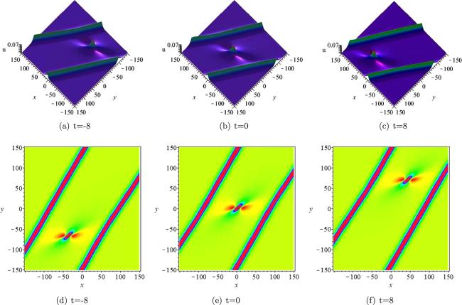
Figure 6. The 3D plots and corresponding density plots of equation ( |
6.3. The periodic cross-kink solutions of equation (1 )
We assume that32 ) into equation (3 ), we obtain33 ) into equation (32 ), we get2 ), we have34 ), appears as two intersecting solitons. Over time, the narrower soliton moves upward to the left, while the wider soliton moves upward to the right. And the intersection of the two solitons moves with time along the positive semi-axis of x and y.
$\begin{eqnarray}f={{\rm{e}}}^{-{\phi }_{3}}+{\delta }_{3}{{\rm{e}}}^{{\phi }_{3}}+{\delta }_{4}\sin \left({\phi }_{4}\right)+{\delta }_{5}\sinh \left({\phi }_{5}\right)+{\eta }_{16},\end{eqnarray}$
where $\begin{eqnarray*}\begin{array}{l}{\phi }_{3}={\eta }_{1}x+{\eta }_{2}y+{\eta }_{3}z+{\eta }_{4}t+{\eta }_{5},\\ {\phi }_{4}={\eta }_{6}x+{\eta }_{7}y+{\eta }_{8}z+{\eta }_{9}t+{\eta }_{10},\\ {\phi }_{5}={\eta }_{11}x+{\eta }_{12}y+{\eta }_{13}z+{\eta }_{14}t+{\eta }_{15}\end{array}\end{eqnarray*}$
and ${\eta }_{i}\left(i=1,\ldots ,16\right)$ is an undetermined constant. Plugging equations ( $\begin{eqnarray}\begin{array}{l}{\eta }_{1}={\eta }_{6}=0,{\eta }_{4}=-\displaystyle \frac{g{\eta }_{2}+h{\eta }_{3}+b{\eta }_{3}{\eta }_{11}^{2}+c{\eta }_{2}{\eta }_{11}^{2}}{a},\\ {\eta }_{9}=-\displaystyle \frac{g{\eta }_{7}+h{\eta }_{8}+b{\eta }_{8}{\eta }_{11}^{2}+c{\eta }_{7}{\eta }_{11}^{2}}{a},\\ {\eta }_{12}=-\displaystyle \frac{b{\eta }_{13}}{c},\,\,\,\,\,\,{\eta }_{14}=\displaystyle \frac{{bg}{\eta }_{13}-{cd}{\eta }_{11}-{ch}{\eta }_{13}}{{ac}},\end{array}\end{eqnarray}$
where a, b, c, d, g, h, η2, η3, η5, η6, η7, η8, η10, η11, η13, η15 and η16 are arbitrary nonzero constants. By substituting equation ( $\begin{eqnarray*}\begin{array}{l}f={{\rm{e}}}^{-\left({\eta }_{2}y+{\eta }_{3}z-\displaystyle \frac{g{\eta }_{2}+h{\eta }_{3}+b{\eta }_{3}{\eta }_{11}^{2}+c{\eta }_{2}{\eta }_{11}^{2}}{a}t+{\eta }_{5}\right)}\\ \quad +{\delta }_{3}{{\rm{e}}}^{{\eta }_{2}y+{\eta }_{3}z-\displaystyle \frac{g{\eta }_{2}+h{\eta }_{3}+b{\eta }_{3}{\eta }_{11}^{2}+c{\eta }_{2}{\eta }_{11}^{2}}{a}t+{\eta }_{5}}\\ +{\delta }_{4}\sin \left({\eta }_{7}y+{\eta }_{8}z-\displaystyle \frac{g{\eta }_{7}+h{\eta }_{8}+b{\eta }_{8}{\eta }_{11}^{2}+c{\eta }_{7}{\eta }_{11}^{2}}{a}t+{\eta }_{10}\right)\\ +{\delta }_{5}\sinh \left({\eta }_{11}x-\displaystyle \frac{b{\eta }_{13}}{c}y+{\eta }_{13}z+\displaystyle \frac{{bg}{\eta }_{13}-{cd}{\eta }_{11}-{ch}{\eta }_{13}}{{ac}}t+{\eta }_{15}\right)\\ \quad +{\eta }_{16},\end{array}\end{eqnarray*}$
then, by virtue of the transformation, equation ( $\begin{eqnarray}\begin{array}{l}u=-\displaystyle \frac{2{\delta }_{5}{\eta }_{11}^{2}\sinh \left({\lambda }_{11}\right)}{{{\rm{e}}}^{-{\lambda }_{9}}+{\delta }_{3}{{\rm{e}}}^{{\lambda }_{9}}+{\delta }_{4}\sin \left({\lambda }_{10}\right)-{\delta }_{5}\sinh \left({\lambda }_{11}\right)+{\eta }_{16}}\\ \quad -\displaystyle \frac{2{\delta }_{5}^{2}{\eta }_{11}^{2}\cosh \left({\lambda }_{11}\right)}{{\left[{{\rm{e}}}^{-{\lambda }_{9}}+{\delta }_{3}{{\rm{e}}}^{{\lambda }_{9}}+{\delta }_{4}\sin \left({\lambda }_{10}\right)-{\delta }_{5}\sinh \left({\lambda }_{11}\right)+{\eta }_{16}\right]}^{2}},\end{array}\end{eqnarray}$
where $\begin{eqnarray*}\begin{array}{l}{\lambda }_{9}={\eta }_{2}y+{\eta }_{3}z-\displaystyle \frac{g{\eta }_{2}+h{\eta }_{3}+b{\eta }_{3}{\eta }_{11}^{2}+c{\eta }_{2}{\eta }_{11}^{2}}{a}t+{\eta }_{5},\\ {\lambda }_{10}={\eta }_{7}y+{\eta }_{8}z-\displaystyle \frac{g{\eta }_{7}+h{\eta }_{8}+b{\eta }_{8}{\eta }_{11}^{2}+c{\eta }_{7}{\eta }_{11}^{2}}{a}t+{\eta }_{10},\\ {\lambda }_{11}={\eta }_{11}x-\displaystyle \frac{b{\eta }_{13}}{c}y+{\eta }_{13}z+\displaystyle \frac{{bg}{\eta }_{13}-{cd}{\eta }_{11}-{ch}{\eta }_{13}}{{ac}}t\\ \quad +{\eta }_{15}.\end{array}\end{eqnarray*}$
We take a = b = c = d = g = h = 1. It can be observed in figure 7 that the solution, equation (
Figure 7. Density plots of equation ( |
7. Conclusion
In this paper, we first consider a generalized (3+1)-dimensional equation, and derive its bilinear form using Hirota’s bilinear method. The lump solutions localized in the whole plane are obtained via the quadratic function method. To analyze the dynamical behavior of the lump waves, three examples are given and the 3D plots and corresponding density plots are presented. It is notable that the method used here to obtain lump solutions can be extended to other (3+1)-dimensional equations. However, the lump solutions derived by this method are localized in the whole plane, but only as single-lump solutions, while the lump solutions obtained via methods such as the long-wave limit are multi-lump solutions, but not necessarily localized in the whole plane. Moreover, the breath-wave solutions, the mixed lump–soliton solutions, the mixed rogue-wave–soliton solutions and the periodic cross-kink solutions are derived. In future work, we will explore whether this method can derive multi-lump solutions localized in the whole plane of the (3+1)-dimensional equations. Recent studies have proved the existence of line rogue waves in some (2+1)-dimensional evolution equations [40, 41]. We will investigate the existence of line rogue waves in (3+1)-dimensional equations in future work.