


1. Introduction
Partial differential equations (PDEs) play a vital role in the study of engineering and applied mathematics, particularly in fluid mechanics and electromagnetics [1–5]. Nonlinear evolution equations (NLEEs) are foremost in the study of nonlinear phenomena. NLEEs are commonly applied to demonstrate the problems of plasma physics, fluid mechanics, biology, optical fibers, chemically reactive materials, chemical kinetics, electricity etc [6–11]. Various methods have been utilized to find the solutions to NLEEs. They include an inverse scattering algorithm, Darboux transformations, Hirota bilinear approach, Lie symmetry analysis (LSA) etc [12–15].
The Lie Group approach, also called LSA, is a successful and fruitful mechanism for attaining the symmetries, exact solutions, and conservation laws (CLs) of NLEEs [16]. It was introduced by the Norwegian mathematician Sophus Lie in 1880. Many NLEEs have been studied under this approach. LSA is used in fractional calculus as well to produce new results. A symmetry of a differential equation (DE) converts one solution to another solution. New solutions can be produced from the older ones with the aid of symmetries of DEs [17]. Symmetries and CLs are a vital part of the study of DEs. The CLs are essential because they provide a mathematical explanation of the model that certain physical quantity like energy, charge, linear, and angular momentum remains unaltered during the evolution of a physical system. An equation is integrable if it possesses CLs. The CLs of fractional PDEs are the amalgamation of works of Ibragimov [18] and Lukashchuk [19].
CLs of a model can be evaluated by various approaches which include Noether's theorem, variational approach, conservation theorem characteristic method, scaling invariance method etc [20–23]. Hussain et al discussed the Burgers–Huxley equation by LSA and found the CLs [24]. Rashidi and Hejazi [25] in their work used LSA to attain the solutions of a fractional integro-differential system called the Vlasov–Maxwell system. Bahi and Hilal [26] used LSA to find the CLs and exact solutions of the generalized time-fractional Korteweg-de Vries-Burgers-like equation. Liu et al used LSA on generalized time-fractional diffusion equations and also derived the CLs and exact solutions of the model [27–32].
Any equation is said to be self-adjoint if its adjoint equation upon substitution is equal to the original equation. CLs have been derived on the basis of self-adjointness. The equations that are nonlinearly self-adjoint can be written in a strictly self-adjoint form with the aid of suitable multipliers. As a result, any linear equation can be expressed in a nonlinear strictly self-adjoint form [33]. An integrable model possesses soliton solutions. A soliton is a wave that retains its shape and velocity on collision with another soliton. Many researchers have worked on finding the soliton solutions of the models [34–40] by different techniques.
In 1952, Alan Turning [41] gave a concept of turning pattern which describes how patterns like stripes and spots can be set up naturally from a homogeneous uniform state. In one of his papers, he pondered over the behavior of the system where two diffusible materials come across each other to form a spatially periodic pattern. Reaction-diffusion systems (DRS) are mathematical models corresponding to physical phenomena. They are frequently used in the alteration in time and space of concentration of one or several chemical products. We can observe DRS in chemistry, biology, physics, etc. In this article, we will acknowledge a simple reaction model for glycolysis known as a Selkov–Schnakenberg (SS) system proposed by Schnakenberg in 1979. It is a chemical reaction with limited cycle behavior involving three stages:1 ) is transformed into the Selkov model [43]. If δ = 0 and σ > 0 equation (1 ) is turned to the Schnakenberg model [44]. The remaining manuscript is organized as follows: In section 2 , LSA is performed for the above-quoted model. In section 3 , CLs have been formulated. In section 4 , the self-adjointness (SA) of the model is discussed. In section 5 , the model is solved by the sub-ordinary differential equations (sub-ODE) approach in detail. In section 6 , we will interpret the solution of the model with their 3D, 2D, and contour profiles for various parameters. Later, section 7 provides results and discussions of our model. At the end, in section 8 , we will wind up the article by providing our conclusion.
$\begin{eqnarray*}P\rightleftharpoons V,T\rightleftharpoons W,2V+W=3V,\end{eqnarray*}$
V, W and P, T are chemical products and chemical sources representing dimensionless concentrations of the reactants. So the SS system is a couple of nonlinear PDEs of the form [42] $\begin{eqnarray}\begin{array}{l}\alpha {R}_{{xx}}+\beta -R+{R}^{2}S+\delta S-{R}_{t}=0,\\ \gamma {S}_{{xx}}+\sigma -{R}^{2}S-\delta S-{S}_{t}=0,\end{array}\end{eqnarray}$
where R(x, t) and S(x, t) represent the concentrations of the two reactants. α and γ are diffusion coefficients of R and S. β, δ ≥ 0, σ > 0. If β = 0 = δ, equation (2. Lie Symmetry Analysis
In this section, our main focus is on LSA for equation (1 ) which is elaborated below. Let us assume we have one parameter Lie Group of point transmformations [45, 46]1 Pr2 will be the second prolongation then the Lie’s invariance condition is
$\begin{eqnarray*}\begin{array}{rcl}\overline{x} & = & x+\epsilon {\xi }^{1}(x,t,R,S)+O({\epsilon }^{2}),\\ \overline{t} & = & t+\epsilon {\xi }^{2}(x,t,R,S)+O({\epsilon }^{2}),\\ \overline{R} & = & R+\epsilon {\eta }_{1}(x,t,R,S)+O({\epsilon }^{2}),\\ \overline{S} & = & S+\epsilon {\eta }_{2}(x,t,R,S)+O({\epsilon }^{2}),\end{array}\end{eqnarray*}$
where ε ≤ 1 is the group parameter. ξ1(x, t, R, S), ξ2(x, t, R, S), η1(x, t, R, S) and η2(x, t, R, S) are the infinitesimal generators which we have to calculate. The vector field associated with the above-mentioned group of transformations is given by $\begin{eqnarray}\begin{array}{l}Y={\xi }^{1}(x,t,R,S)+\displaystyle \frac{\partial }{\partial x}+{\xi }^{2}(x,t,R,S)\displaystyle \frac{\partial }{\partial t}\\ \quad +{\eta }_{1}(x,t,R,S)\displaystyle \frac{\partial }{\partial R}+{\eta }_{2}(x,t,R,S)\displaystyle \frac{\partial }{\partial S}.\end{array}\end{eqnarray}$
For system $\begin{eqnarray*}\begin{array}{l}{{\Pr }}^{2}Y({\bigtriangleup }_{1}){| }_{{\bigtriangleup }_{1}=0,{\bigtriangleup }_{2}=0}=0,\\ {{\Pr }}^{2}Y({\bigtriangleup }_{2}){| }_{{\bigtriangleup }_{1}=0,{\bigtriangleup }_{2}=0}=0,\end{array}\end{eqnarray*}$
where $\begin{eqnarray}{\bigtriangleup }_{1}=\alpha {R}_{{xx}}+\beta -R+{R}^{2}S+\delta S,\end{eqnarray}$
$\begin{eqnarray}{\bigtriangleup }_{2}=\gamma {S}_{{xx}}+\sigma -{R}^{2}S-\delta S.\end{eqnarray}$
Using SYM package launched by Dimas and Tsoubelis [47] we get the determining equations which are obtained by equating the polynomials to zero. Solution of these determining equations give values of ξ1(x, t, R, S), ξ2(x, t, R, S), η1(x, t, R, S) and η2(x, t, R, S) asCase (i): When
α = 0, γ = 0 and RS ≠ 0.
$\begin{eqnarray}\begin{array}{l}{\eta }_{1}(x,t,R,S)=-\displaystyle \frac{1}{2{RS}}\left((\delta +{R}^{2}){\eta }_{2}(x,t,R,S)+(-{R}^{2}S+\sigma -\delta S){\eta }_{2,S}\right.\\ \quad -{R}^{4}{S}^{2}{\xi }_{S}^{2}-2\delta {R}^{2}{S}^{2}{\xi }_{S}^{2}-{\delta }^{2}{S}^{2}{\xi }_{S}^{2}+2{R}^{2}\sigma S{\xi }_{S}^{2}+2\delta \sigma S{\xi }_{S}^{2}\\ \quad -{\sigma }^{2}{\xi }_{S}^{2}-R{\eta }_{2,R}+{R}^{2}S{\eta }_{2,R}+\beta {\eta }_{2,R}+S\delta {\eta }_{2,R}-{R}^{3}S{\xi }_{R}^{2}\\ \quad +{R}^{4}{S}^{2}{\xi }_{R}^{2}+\beta {R}^{2}S{\xi }_{R}^{2}-\delta (R)S{\xi }_{R}^{2}+2\delta {R}^{2}{S}^{2}{\xi }_{R}^{2}\\ \quad +\beta \delta S{\xi }_{R}^{2}+{\delta }^{2}{S}^{2}{\xi }_{R}^{2}+R\sigma {\xi }_{R}^{2}-{R}^{2}\sigma S{\xi }_{R}^{2}-\beta \sigma {\xi }_{R}^{2}\\ \quad \left.-\delta \sigma S{\xi }_{R}^{2}+{\eta }_{2,t}+{R}^{2}S{\xi }_{t}^{2}+\delta S{\xi }_{t}^{2}-\sigma {\xi }_{t}^{2}\right).\end{array}\end{eqnarray}$
Case (ii): Whenα = 0 and (γδR3σ + γδ2Rσ ≠ 0),
α = 0, δ = 0 and γRσ ≠ 0,
α = 0, σ = 0 and γR ≠ 0.
$\begin{eqnarray}{\xi }^{1}(x,t,R,S)={c}_{1}+{c}_{3},\end{eqnarray}$
$\begin{eqnarray}{\xi }^{2}(x,t,R,S)={c}_{2},\end{eqnarray}$
$\begin{eqnarray}{\eta }_{1}(x,t,R,S)=0,\end{eqnarray}$
$\begin{eqnarray}{\eta }_{2}(x,t,R,S)=0.\end{eqnarray}$
Case (iii): When
γ = α and $(\alpha \beta {\delta }^{2}\sigma -\alpha \beta \delta \sigma {\cot }^{2}(1)\ne 0),$
β = 0, γ = α and $(\alpha {\delta }^{2}\sigma -\alpha \delta \sigma {\cot }^{2}(1)\ne 0),$
$\gamma =\alpha ,\delta ={\cot }^{2}(1)$ and αRσ ≠ 0,
γ = α, σ = 0 and $(\alpha {\delta }^{3}-\alpha {\delta }^{2}{\cot }^{2}(1)+\alpha {\delta }^{2}{R}^{2}-\alpha \delta {R}^{2}{\cot }^{2}(1)\ne 0),$
$\gamma =\alpha ,\delta ={\cot }^{2}(1),\sigma =0$ and $\alpha {\cot }^{2}(1)+\alpha {R}^{2}\ne 0).$
$\begin{eqnarray}{\xi }^{1}(x,t,R,S)={c}_{2},\end{eqnarray}$
$\begin{eqnarray}{\xi }^{2}(x,t,R,S)={c}_{1},\end{eqnarray}$
$\begin{eqnarray}{\eta }_{1}(x,t,R,S)=0,\end{eqnarray}$
$\begin{eqnarray}{\eta }_{2}(x,t,R,S)=0.\end{eqnarray}$
Case (iv): Whenγ = 0 and (αδ2 + αδR2 ≠ 0),
γ = 0, δ = 0, αβR ≠ 0,
β = 0, γ = 0, δ = 0 and αR ≠ 0.
$\begin{eqnarray}{\xi }^{1}(x,t,R,S)={c}_{2}+{c}_{3},\end{eqnarray}$
$\begin{eqnarray}{\xi }^{2}(x,t,R,S)={c}_{1},\end{eqnarray}$
$\begin{eqnarray}{\eta }_{1}(x,t,R,S)=0,\end{eqnarray}$
$\begin{eqnarray}{\eta }_{2}(x,t,R,S)=0.\end{eqnarray}$
Case (v): Whenδ = 0 and α2βγRσ − αβγ2Rσ ≠ 0),
σ = 0 and (α2γδR4 − αγ2δR4 − α2βγδR3 + αβγ2δR3 + α2γδ2R2 − αγ2δ2R2 − α2βγδ2R + αβγ2δ2R ≠ 0),
β = 0, δ = 0 and α2γRσ − αγ2Rσ ≠ 0),
δ = 0, σ = 0 and α2βγR − αβγ2R ≠ 0),
β = 0, δ = 0, σ = 0 and (α2γR − αγ2R ≠ 0),
αγδσ(α − γ)(R2 − δ) ≠ 0. 1 ) is spanned by the linearly independent operators
$\begin{eqnarray}{\xi }^{1}(x,t,R,S)={c}_{1},\end{eqnarray}$
$\begin{eqnarray}{\xi }^{2}(x,t,R,S)={c}_{2},\end{eqnarray}$
$\begin{eqnarray}{\eta }_{1}(x,t,R,S)=0,\end{eqnarray}$
$\begin{eqnarray}{\eta }_{2}(x,t,R,S)=0,\end{eqnarray}$
where c1, c2 and c3 are constants. The Lie symmetry algebra introduced by equation ( $\begin{eqnarray}{Y}_{1}={\partial }_{x},\end{eqnarray}$
$\begin{eqnarray}{Y}_{2}={\partial }_{y}.\end{eqnarray}$
3. Conservation laws
In this section, we compute CLs [45] for the SS system by a new procedure that is based on the formal Lagrangian [48]. The conserved vectors for each symmetry are established below. The Lagrangian is given by
$\begin{eqnarray*}\begin{array}{l}L=z(x,t)(\beta -R(x,t)+\delta S(x,t)+{R}^{2}(x,t)S(x,t)\\ \quad -{R}_{t}+\alpha {R}_{{xx}}(x,t))+w(x,t)(\sigma -\delta S(x,t)\\ \quad -{R}^{2}(x,t)S(x,t)-{S}_{t}(x,t)+\gamma {S}_{{xx}}(x,t)),\end{array}\end{eqnarray*}$
where z(x, t) = RB1 and w(x, t) = − SB1. B1 ia an arbitrary constant.For symmetry Y1, the conserved vectors are
$\begin{eqnarray}{Y}_{1}^{x}={\rm{B}}1\left(R\beta -S\sigma -{R}^{2}(x,t)+(R+S)\delta S(x,t)+(R+S)R{\left(x,t\right)}^{2}S(x,t)-{{RR}}_{t}+{{SS}}_{t}\right)\end{eqnarray}$
$\begin{eqnarray}{Y}_{1}^{t}={\rm{B}}1\left({{RR}}_{x}-{{SS}}_{x}\right).\end{eqnarray}$
For symmetry Y2, the conserved vectors are: $\begin{eqnarray}{Y}_{2}^{x}=-{\rm{B}}1R\alpha {R}_{{xt}}+{\rm{B}}1S\gamma {S}_{{xt}},\end{eqnarray}$
$\begin{aligned} Y_{2}^{t} & =\mathrm{B} 1\left(R \beta-S \sigma-R^{2}(x, t)+(R+S) \delta S(x, t)\right. \\ & \left.+(R+S) R(x, t)^{2} S(x, t)+R \alpha R_{x x}-S \gamma S_{x x}\right) . \end{aligned}$
4. Self adjointness
Let us assume a system of DEs with $\overline{p}$ equations with p dependent variables and g = (g1,…,gp)[49].28 ) upon replacing
$\begin{eqnarray}{M}_{\overline{\alpha }}(x,g,{g}_{(1)},\ldots ,{g}_{(n)})=0,\hspace{0.5cm}\overline{\alpha }=1,2,\ldots ,\overline{p}.\end{eqnarray}$
This system is said to have nonlinearly SA if the succeeding adjoint equations $\begin{eqnarray}\begin{array}{l}{M}_{\alpha }^{* }(x,g,{g}_{(1)},{h}_{(1)},\ldots ,{g}_{(n)},{h}_{(n)})\equiv \delta ({h}^{\overline{{\rm{\Omega }}}}{M}_{\overline{{\rm{\Omega }}}})/\delta {g}^{\alpha }=0,\\ \alpha =1,2,\ldots ,p.\end{array}\end{eqnarray}$
are satisfied for all solutions g of the system ( $\begin{eqnarray}{h}^{\overline{\alpha }}={\psi }^{\overline{\alpha }}(x,g),\hspace{0.5cm}\overline{\alpha }=1,2,\ldots ,\overline{p}.\end{eqnarray}$
such that $\begin{eqnarray}\psi (x,g)\ne 0.\end{eqnarray}$
4.1. Nonlinear self adjointness of the Selkov–Schnakenberg system
Our main aim is to show that equation (1 ) is nonlinearly SA. The adjoint equation for equation (1 ) is stated as
$\begin{eqnarray}\begin{array}{l}2R(x,t)S(x,t)(-w(x,t)+z(x,t))+{z}_{t}+\alpha {z}_{{xx}}=z(x,t),\\ \left(\delta +{R}^{2}(x,t)\right)(w(x,t)-z(x,t))={w}_{t}+\gamma {w}_{{xx}}.\end{array}\end{eqnarray}$
Suppose z = Z(x, t, R, S) and w = W(x, t, R, S), after performing a few calculations the following equation is attained $\begin{eqnarray*}\begin{array}{l}2R(x,t)S(x,t)(-W(x,t,R,S)+Z(x,t,R,S))+{S}_{t}{Z}_{S}\\ \quad +\alpha {Z}_{{SS}}{S}_{x}{}^{2}+{R}_{t}{Z}_{R}+2\alpha {R}_{x}{S}_{x}{Z}_{{RS}}+\alpha {Z}_{R}{R}_{{xx}}\\ \quad +\alpha {Z}_{S}{S}_{{xx}}+\alpha {R}_{x}^{2}{Z}_{{RR}}=Z(x,t,R,S),\end{array}\end{eqnarray*}$
$\begin{eqnarray*}\begin{array}{l}(\delta +{R}^{2}(x,t))(W(x,t,R,S)-Z(x,t,R,S))={S}_{t}{W}_{S}\\ \quad +\gamma {W}_{{SS}}{S}_{x}^{2}+{R}_{t}{W}_{R}+2\gamma {R}_{x}{S}_{x}{W}_{{RS}}+\gamma {W}_{R}{R}_{{xx}}\\ \quad +\gamma {W}_{S}{S}_{{xx}}+\gamma {R}_{x}^{2}{W}_{{RR}}.\end{array}\end{eqnarray*}$
Now equating the coefficients of Rt, St, Rx, Sx, Rxx, Sxx to zero, we obtain1 ) is a nonlinearly SA with the substitution equation given by equation (33 ).
$\begin{eqnarray}\begin{array}{l}-(\delta +{R}^{2}(x,t)(W(x,t,R,S)-Z(x,t,R,S))={S}_{t}{W}_{S}+\gamma {W}_{{SS}}{S}_{x}{}^{2}\\ \quad +{R}_{t}{W}_{R}+2\gamma {R}_{x}{S}_{x}{W}_{{RS}}+\gamma {W}_{R}{R}_{{xx}}\\ \quad +\gamma {W}_{S}{S}_{{xx}}+\gamma {R}_{x}{}^{2}{W}_{{RR}})+(2R(x,t)S(x,t)(-W(x,t,R,S)+Z(x,t,R,S))+{S}_{t}{Z}_{S}\\ \,+\alpha {Z}_{{SS}}{S}_{x}{}^{2}\\ \quad +{R}_{t}{Z}_{R}+2\alpha {R}_{x}{S}_{x}{Z}_{{RS}}+\alpha {Z}_{R}{R}_{{xx}}+\alpha {Z}_{S}{S}_{{xx}}+\alpha {R}_{x}{}^{2}{Z}_{{RR}}=Z(x,t,R,S))=0.\end{array}\end{eqnarray}$
The solution of Z(x, t, R, S) and W(x, t, R, S) is found to be $\begin{eqnarray}\begin{array}{rcl}Z & = & {{RB}}_{1},\\ W & = & -{{SB}}_{1},\end{array}\end{eqnarray}$
where B1 is any constant. Hence, equation (5. Sub-ODE technique
In this section, the soliton solutions of SS equation (1 ) will be obtained via a sub-ODE mechanism by the assumption [50],5 ) and equation (35 ) in equation (1 ) we achieve a system of ODEs36 ) we get38 ) has a solution38 )38 ) is given as:41 ) together with equation (43 ) in equation (38 ) and equating the coefficients of powers of G we arrive at the following equations:
$\begin{eqnarray*}R(x,t)=A(\psi ),\quad S(x,t)=B(\psi ).\end{eqnarray*}$
and $\begin{eqnarray}\psi ={qx}-{ct}.\end{eqnarray}$
where c is the non-zero velocity of the soliton, A(ψ) and B(ψ) are real functions explaining the appearance of the solitary wave. Inserting equation ( $\begin{eqnarray}\begin{array}{l}{cA}^{\prime} +{q}^{2}\alpha A^{\prime\prime} +\beta -A+{A}^{2}B+\delta B=0,\\ {cB}^{\prime} +{q}^{2}\gamma B^{\prime\prime} +\sigma -{A}^{2}B-\delta B=0.\end{array}\end{eqnarray}$
Now putting $\begin{eqnarray}B(\psi )=\eta A(\psi ),\qquad \eta \ne 0.\end{eqnarray}$
In equation ( $\begin{eqnarray}{cA}^{\prime} +{q}^{2}\alpha A^{\prime\prime} +\beta -A+\eta {A}^{3}+\delta \eta A=0,\end{eqnarray}$
$\begin{eqnarray}c\eta A^{\prime} +{q}^{2}\gamma \eta A^{\prime\prime} +\sigma -\eta {A}^{3}+\delta \eta A=0.\end{eqnarray}$
As stated in the sub-ODE algorithm, we presume that ( $\begin{eqnarray}A(\psi )=\mu {G}^{m}(\psi ),\,\,\,\,\,\,\mu \gt 0,\end{eqnarray}$
where m is a parameter and G(ψ) satisfies the equation $\begin{eqnarray}\begin{array}{l}G{{\prime} }^{2}(\psi )={{JG}}^{2-2p}(\psi )+{{HG}}^{2-p}(\psi )+{{LG}}^{2}(\psi )\\ \quad +{{MG}}^{2+p}(\psi )+{{QG}}^{2+2p}(\psi ),\,\,\,\,\,\,\,p\gt 0,\end{array}\end{eqnarray}$
where J, H, L, M, and Q are constants and m is found by the homogeneous balance method [50] between A″ and A3 in equation ( $\begin{eqnarray}m+2p=3m\Longrightarrow p=m,\end{eqnarray}$
Now the solution of equation ( $\begin{eqnarray}A(\psi )=\mu {G}^{p}(\psi ).\end{eqnarray}$
Substituting equation ( $\begin{eqnarray}\begin{array}{l}{G}^{0}(\psi ):\beta +\displaystyle \frac{1}{2}\alpha H\mu {p}^{2}{q}^{2}=0,\\ {G}^{p}(\psi ):-\mu +\alpha \mu {{Lp}}^{2}{q}^{2}+\delta \eta \mu =0,\\ {G}^{2p}(\psi ):\displaystyle \frac{3}{2}\alpha \mu {{Mp}}^{2}{q}^{2}=0,\\ {G}^{3p}(\psi ):2\alpha \mu {p}^{2}{q}^{2}Q+\eta {\mu }^{3}=0.\end{array}\end{eqnarray}$
Type 1. Substituting J = H = M = 0 in equation (44 ) we have45 ) along with equation (25) of [50] in equation (43 ) we obtain the bright soliton solution of equation (1 ) as45 ) along with equation (26) of [50] in equation (43 ) we achieve the periodic solution of equation (1 ) as45 ) along with equation (27) of [50] in equation (43 ) we get the rational solution of equation (1 )
$\begin{eqnarray}\mu =\sqrt{\displaystyle \frac{-2Q\alpha }{\eta }}{pq},\,\,\,\,\,\,\,\,\,\,\,\,L=\displaystyle \frac{1-\delta \eta }{{p}^{2}{q}^{2}\alpha }.\end{eqnarray}$
Using equation ( $\begin{eqnarray}\begin{array}{l}{A}_{1}(x,t)=\sqrt{2}{pq}\sqrt{-\displaystyle \frac{\alpha Q}{\eta }}\sqrt{\displaystyle \frac{\delta \eta -1}{\alpha {p}^{2}{q}^{2}Q}}\\ \quad \times \,{\rm{sech}} \left(p({qx}-{ct})\sqrt{\displaystyle \frac{1-\delta \eta }{\alpha {p}^{2}{q}^{2}}}\right),\end{array}\end{eqnarray}$
$\begin{eqnarray}\begin{array}{l}{B}_{1}(x,t)=\sqrt{2}\eta {pq}\sqrt{-\displaystyle \frac{\alpha Q}{\eta }}\sqrt{\displaystyle \frac{\delta \eta -1}{\alpha {p}^{2}{q}^{2}Q}}\\ \quad \times \,{\rm{sech}} \left(p({qx}-{ct})\sqrt{\displaystyle \frac{1-\delta \eta }{\alpha {p}^{2}{q}^{2}}}\right).\end{array}\end{eqnarray}$
Using equation ( $\begin{eqnarray}\begin{array}{l}{A}_{2}(x,t)=\sqrt{2}{pq}\sqrt{-\displaystyle \frac{\alpha Q}{\eta }}\sqrt{\displaystyle \frac{\delta \eta -1}{\alpha {p}^{2}{q}^{2}Q}}\\ \quad \times \,\sec \left(p({qx}-{ct})\sqrt{\displaystyle \frac{\delta \eta -1}{\alpha {p}^{2}{q}^{2}}}\right),\end{array}\end{eqnarray}$
$\begin{eqnarray}\begin{array}{l}{B}_{2}(x,t)=\sqrt{2}\eta {pq}\sqrt{-\displaystyle \frac{\alpha Q}{\eta }}\sqrt{\displaystyle \frac{\delta \eta -1}{\alpha {p}^{2}{q}^{2}Q}}\\ \quad \times \,\sec \left(p({qx}-{ct})\sqrt{\displaystyle \frac{\delta \eta -1}{\alpha {p}^{2}{q}^{2}}}\right).\end{array}\end{eqnarray}$
Using equation ( $\begin{eqnarray}{A}_{3}(x,t)=\displaystyle \frac{\sqrt{2}q\epsilon \sqrt{-\tfrac{\alpha Q}{\eta }}}{\sqrt{Q}({qx}-{ct})},\end{eqnarray}$
$\begin{eqnarray}{B}_{3}(x,t)=\displaystyle \frac{\sqrt{2}\eta q\epsilon \sqrt{-\tfrac{\alpha Q}{\eta }}}{\sqrt{Q}({qx}-{ct})}.\end{eqnarray}$
given that $\tfrac{\alpha Q}{\eta }\lt 0,\tfrac{\delta \eta -1}{\alpha {p}^{2}{q}^{2}Q}\gt 0.$Type 2. Putting $H=M=0,J=\tfrac{{L}^{2}}{4Q}$ in equation (44 ) we obtain52 ) along with equation (28) of [50] in equation (43 ) we get the dark soliton solution of equation (1 ) as52 ) along with equation (29) of [50] in equation (43 ) the periodic solution is given by
$\begin{eqnarray}\mu =\sqrt{2}{pq}\sqrt{-\displaystyle \frac{\alpha Q}{\eta }},\,\,\,\,\,\,\,\,L=\displaystyle \frac{1-\delta \eta }{{p}^{2}{q}^{2}\alpha }.\end{eqnarray}$
Using equation ( $\begin{eqnarray}\begin{array}{l}{A}_{4}(x,t)=\sqrt{2}{pq}\epsilon \sqrt{-\displaystyle \frac{\alpha Q}{\eta }}\sqrt{\displaystyle \frac{\delta \eta -1}{\alpha {p}^{2}{q}^{2}Q}}\\ \quad \times \,\tanh \left(p({qx}-{ct})\sqrt{\displaystyle \frac{1-\delta \eta }{\alpha {p}^{2}{q}^{2}}}\right),\end{array}\end{eqnarray}$
$\begin{eqnarray}\begin{array}{l}{B}_{4}(x,t)=\sqrt{2}\eta {pq}\epsilon \sqrt{-\displaystyle \frac{\alpha Q}{\eta }}\sqrt{\displaystyle \frac{\delta \eta -1}{\alpha {p}^{2}{q}^{2}Q}}\\ \quad \times \,\tanh \left(p({qx}-{ct})\sqrt{\displaystyle \frac{1-\delta \eta }{\alpha {p}^{2}{q}^{2}}}\right).\end{array}\end{eqnarray}$
Using equation ( $\begin{eqnarray}\begin{array}{l}{A}_{5}(x,t)=\sqrt{2}{pq}\epsilon \sqrt{-\displaystyle \frac{\alpha Q}{\eta }}\sqrt{\displaystyle \frac{\delta \eta -1}{\alpha {p}^{2}{q}^{2}Q}}\\ \quad \times \,\tan \left(p({qx}-{ct})\sqrt{\displaystyle \frac{\delta \eta -1}{\alpha {p}^{2}{q}^{2}}}\right),\end{array}\end{eqnarray}$
$\begin{eqnarray}\begin{array}{l}{B}_{5}(x,t)=\sqrt{2}\eta {pq}\epsilon \sqrt{-\displaystyle \frac{\alpha Q}{\eta }}\sqrt{\displaystyle \frac{\delta \eta -1}{\alpha {p}^{2}{q}^{2}Q}}\\ \quad \times \,\tan \left(p({qx}-{ct})\sqrt{\displaystyle \frac{\delta \eta -1}{\alpha {p}^{2}{q}^{2}}}\right).\end{array}\end{eqnarray}$
provided that $\tfrac{\alpha Q}{\eta }\lt 0,\tfrac{\delta \eta -1}{\alpha {p}^{2}{q}^{2}Q}\gt 0.$Type 3. Putting H = M = 0 in equation (44 ) we obtain57 ) along with equation (30) of [50] in equation (43 ) we get the Jacobian elliptic solutions of equation (1 ) as58 ) is converted to:58 ) is converted to:57 ) along with equation (31) of [50] in equation (43 ) we get63 ) is converted to:57 ) along with equation (32) of [50] in equation (43 ) we get66 ) is converted to:
$\begin{eqnarray}\mu =\sqrt{2}{pq}\sqrt{-\displaystyle \frac{\alpha Q}{\eta }},\,\,\,\,\,\,\,\,L=\displaystyle \frac{1-\delta \eta }{{p}^{2}{q}^{2}\alpha }.\end{eqnarray}$
Using equation ( $\begin{eqnarray*}\begin{array}{l}{A}_{6}(x,t)=\sqrt{2}{pq}\sqrt{-\displaystyle \frac{\alpha Q}{\eta }}\sqrt{\displaystyle \frac{{m}^{2}(\delta \eta -1)}{\alpha \left(2{m}^{2}-1\right){p}^{2}{q}^{2}Q}}\\ \quad \times \,\mathrm{cn}\left(p({qx}-{ct})\sqrt{\displaystyle \frac{1-\delta \eta }{\alpha \left(2{m}^{2}-1\right){p}^{2}{q}^{2}}}\right),\end{array}\end{eqnarray*}$
$\begin{eqnarray}\begin{array}{l}{B}_{6}(x,t)=\sqrt{2}\eta {pq}\sqrt{-\displaystyle \frac{\alpha Q}{\eta }}\sqrt{-\displaystyle \frac{{m}^{2}(1-\delta \eta )}{\alpha \left(2{m}^{2}-1\right){p}^{2}{q}^{2}Q}}\\ \quad \times \,\mathrm{cn}\left(p({qx}-{ct})\sqrt{\displaystyle \frac{1-\delta \eta }{\alpha \left(2{m}^{2}-1\right){p}^{2}{q}^{2}}}\right).\end{array}\end{eqnarray}$
When m → 0, then equation ( $\begin{eqnarray}\begin{array}{l}{A}_{7}(x,t)=\sqrt{2}{pq}\sqrt{-\displaystyle \frac{\alpha Q}{\eta }}\sqrt{\displaystyle \frac{{m}^{2}(\delta \eta -1)}{\alpha \left(2{m}^{2}-1\right){p}^{2}{q}^{2}Q}}\\ \quad \times \,\cos \left(p({qx}-{ct})\sqrt{\displaystyle \frac{1-\delta \eta }{\alpha \left(2{m}^{2}-1\right){p}^{2}{q}^{2}}}\right),\end{array}\end{eqnarray}$
$\begin{eqnarray}\begin{array}{l}{B}_{7}(x,t)=\sqrt{2}\eta {pq}\sqrt{-\displaystyle \frac{\alpha Q}{\eta }}\sqrt{-\displaystyle \frac{{m}^{2}(1-\delta \eta )}{\alpha \left(2{m}^{2}-1\right){p}^{2}{q}^{2}Q}}\\ \quad \times \,\cos \left(p({qx}-{ct})\sqrt{\displaystyle \frac{1-\delta \eta }{\alpha \left(2{m}^{2}-1\right){p}^{2}{q}^{2}}}\right).\end{array}\end{eqnarray}$
When m → 1, then equation ( $\begin{eqnarray}\begin{array}{l}{A}_{8}(x,t)=\sqrt{2}{pq}\sqrt{-\displaystyle \frac{\alpha Q}{\eta }}\sqrt{\displaystyle \frac{{m}^{2}(\delta \eta -1)}{\alpha \left(2{m}^{2}-1\right){p}^{2}{q}^{2}Q}}\\ \quad \times \,{\rm{sech}} \left(p({qx}-{ct})\sqrt{\displaystyle \frac{1-\delta \eta }{\alpha \left(2{m}^{2}-1\right){p}^{2}{q}^{2}}}\right),\end{array}\end{eqnarray}$
$\begin{eqnarray}\begin{array}{l}{B}_{8}(x,t)=\sqrt{2}\eta {pq}\sqrt{-\displaystyle \frac{\alpha Q}{\eta }}\sqrt{-\displaystyle \frac{{m}^{2}(1-\delta \eta )}{\alpha \left(2{m}^{2}-1\right){p}^{2}{q}^{2}Q}}\\ \quad \times \,{\rm{sech}} \left(p(({qx}-{ct})\sqrt{\displaystyle \frac{1-\delta \eta }{\alpha \left(2{m}^{2}-1\right){p}^{2}{q}^{2}}}\right).\end{array}\end{eqnarray}$
Using equation ( $\begin{eqnarray*}\begin{array}{l}{A}_{9}(x,t)=\sqrt{2}{pq}\sqrt{-\displaystyle \frac{\alpha Q}{\eta }}\sqrt{\displaystyle \frac{1-\delta \eta }{\alpha \left({m}^{2}-2\right){p}^{2}{q}^{2}Q}}\\ \quad \times \,\mathrm{dn}\left(p({qx}-{ct})\sqrt{\displaystyle \frac{\delta \eta -1}{\alpha \left({m}^{2}-2\right){p}^{2}{q}^{2}}}\right),\end{array}\end{eqnarray*}$
$\begin{eqnarray}\begin{array}{l}{B}_{9}(x,t)=\sqrt{2}\eta {pq}\sqrt{-\displaystyle \frac{\alpha Q}{\eta }}\sqrt{-\displaystyle \frac{1-\delta \eta }{\alpha \left(2-{m}^{2}\right){p}^{2}{q}^{2}Q}}\\ \quad \times \,\mathrm{dn}\left(p({qx}-{ct})\sqrt{\displaystyle \frac{1-\delta \eta }{\alpha \left(2-{m}^{2}\right){p}^{2}{q}^{2}}}\right).\end{array}\end{eqnarray}$
When m → 1, then equation ( $\begin{eqnarray}\begin{array}{l}{A}_{10}(x,t)=\sqrt{2}{pq}\sqrt{-\displaystyle \frac{\alpha Q}{\eta }}\sqrt{\displaystyle \frac{1-\delta \eta }{\alpha \left({m}^{2}-2\right){p}^{2}{q}^{2}Q}}\\ \quad \times \,{\rm{sech}} \left(p({qx}-{ct})\sqrt{\displaystyle \frac{\delta \eta -1}{\alpha \left({m}^{2}-2\right){p}^{2}{q}^{2}}}\right),\end{array}\end{eqnarray}$
$\begin{eqnarray}\begin{array}{l}{B}_{10}(x,t)=\sqrt{2}\eta {pq}\sqrt{-\displaystyle \frac{\alpha Q}{\eta }}\sqrt{-\displaystyle \frac{1-\delta \eta }{\alpha \left(2-{m}^{2}\right){p}^{2}{q}^{2}Q}}\\ \quad \times \,{\rm{sech}} \left(p({qx}-{ct})\sqrt{\displaystyle \frac{1-\delta \eta }{\alpha \left(2-{m}^{2}\right){p}^{2}{q}^{2}}}\right).\end{array}\end{eqnarray}$
Using equation ( $\begin{eqnarray*}\begin{array}{l}{A}_{11}(x,t)=\sqrt{2}{pq}\sqrt{-\displaystyle \frac{\alpha Q}{\eta }}\sqrt{\displaystyle \frac{{m}^{2}(\delta \eta -1)}{\alpha \left({m}^{2}+1\right){p}^{2}{q}^{2}Q}}\\ \quad \times \,\mathrm{sn}\left(p({qx}-{ct})\sqrt{\displaystyle \frac{\delta \eta -1}{\alpha \left({m}^{2}+1\right){p}^{2}{q}^{2}}}\right),\end{array}\end{eqnarray*}$
$\begin{eqnarray}\begin{array}{l}{B}_{11}(x,t)=\sqrt{2}\eta {pq}\sqrt{-\displaystyle \frac{\alpha Q}{\eta }}\sqrt{-\displaystyle \frac{{m}^{2}(1-\delta \eta )}{\alpha \left({m}^{2}+1\right){p}^{2}{q}^{2}Q}}\\ \quad \times \,\mathrm{sn}\left(p({qx}-{ct})\sqrt{-\displaystyle \frac{1-\delta \eta }{\alpha \left({m}^{2}+1\right){p}^{2}{q}^{2}}}\right).\end{array}\end{eqnarray}$
When m → 0, then equation ( $\begin{eqnarray}\begin{array}{l}{A}_{12}(x,t)=\sqrt{2}{pq}\sqrt{-\displaystyle \frac{\alpha Q}{\eta }}\sqrt{\displaystyle \frac{{m}^{2}(\delta \eta -1)}{\alpha \left({m}^{2}+1\right){p}^{2}{q}^{2}Q}}\\ \quad \times \,\sin \left(p({qx}-{ct})\sqrt{\displaystyle \frac{\delta \eta -1}{\alpha \left({m}^{2}+1\right){p}^{2}{q}^{2}}}\right),\end{array}\end{eqnarray}$
$\begin{eqnarray}\begin{array}{l}{B}_{12}(x,t)=\sqrt{2}\eta {pq}\sqrt{-\displaystyle \frac{\alpha Q}{\eta }}\sqrt{-\displaystyle \frac{{m}^{2}(1-\delta \eta )}{\alpha \left({m}^{2}+1\right){p}^{2}{q}^{2}Q}}\\ \quad \times \,\sin \left(p({qx}-{ct})\sqrt{-\displaystyle \frac{1-\delta \eta }{\alpha \left({m}^{2}+1\right){p}^{2}{q}^{2}}}\right).\end{array}\end{eqnarray}$
provided that $\tfrac{\alpha Q}{\eta }\lt 0,\tfrac{{m}^{2}(1-\delta \eta )}{\alpha \left({m}^{2}+1\right){p}^{2}{q}^{2}Q}\lt 0.$Type 4. Putting J = H = Q = 0 in equation (44 ) we attain69 ) along with equation (33) of [50] in equation (43 ) we get the bright soliton solution of equation (1 ) as69 ) along with equation (34) of [50] in equation (43 ) we get the periodic solution of equation (1 ) as
$\begin{eqnarray}\mu =\mu ,\,\,\,\,\,\,\,\,L=\displaystyle \frac{1-\delta \eta }{{p}^{2}{q}^{2}\alpha }.\end{eqnarray}$
Using equation ( $\begin{eqnarray}{A}_{13}(x,t)=\displaystyle \frac{\mu (\delta \eta -1){{\rm{sech}} }^{2}\left(\tfrac{p({qx}-{ct})\sqrt{\tfrac{1-\delta \eta }{\alpha {p}^{2}{q}^{2}}}}{\sqrt{2}}\right)}{\alpha {{Mp}}^{2}{q}^{2}},\end{eqnarray}$
$\begin{eqnarray}{B}_{13}(x,t)=-\displaystyle \frac{\eta \mu (1-\delta \eta ){{\rm{sech}} }^{2}\left(\tfrac{p({qx}-{ct})\sqrt{\tfrac{1-\delta \eta }{\alpha {p}^{2}{q}^{2}}}}{\sqrt{2}}\right)}{\alpha {{Mp}}^{2}{q}^{2}}.\end{eqnarray}$
Using equation ( $\begin{eqnarray}{A}_{14}(x,t)=\displaystyle \frac{\mu (\delta \eta -1){\sec }^{2}\left(\tfrac{p({qx}-{ct})\sqrt{\tfrac{\delta \eta -1}{\alpha {p}^{2}{q}^{2}}}}{\sqrt{2}}\right)}{\alpha {{Mp}}^{2}{q}^{2}},\end{eqnarray}$
$\begin{eqnarray}{B}_{14}(x,t)=-\displaystyle \frac{\eta \mu (1-\delta \eta ){\sec }^{2}\left(\tfrac{p({qx}-{ct})\sqrt{-\tfrac{1-\delta \eta }{\alpha {p}^{2}{q}^{2}}}}{\sqrt{2}}\right)}{\alpha {{Mp}}^{2}{q}^{2}}.\end{eqnarray}$
Type 5. Putting L = Q = 0 in equation (44 ) we attain74 ) along with equation (36) of [50] in equation (43 ) we get various Weierstrass elliptic solutions of equation (1 ) as
$\begin{eqnarray}\mu =\sqrt{\displaystyle \frac{-2\beta }{H\alpha }\displaystyle \frac{1}{{pq}}},\,\,\,\,\,\,\,\,\eta =\displaystyle \frac{1}{\delta }.\end{eqnarray}$
Using equation ( $\begin{eqnarray}{A}_{15}(x,t)=\displaystyle \frac{\sqrt{2}\sqrt{-\tfrac{\beta }{\alpha H}}\wp \left(\tfrac{1}{2}\sqrt{M}p({qx}-{ct}),\tfrac{4H}{M},0\right)}{{pq}},\end{eqnarray}$
$\begin{eqnarray}{B}_{15}(x,t)=\displaystyle \frac{\sqrt{2}\eta \sqrt{-\tfrac{\beta }{\alpha H}}\wp \left(\tfrac{1}{2}\sqrt{M}p({qx}-{ct}),\tfrac{4H}{M},0\right)}{{pq}}.\end{eqnarray}$
provided that pq ≠ 0 , $\tfrac{\beta }{H\alpha }\lt 0.$Putting H = M = 0 in equation (44 ) we attain77 ) along with equation (37) of [50] in equation (43 ) we get more Weierstrass elliptic solutions of equation (1 ) as77 ) along with equation (41) of [50] in equation (43 ) we get
$\begin{eqnarray}\mu =\sqrt{\displaystyle \frac{-2Q\alpha }{\eta }}{pq},\,\,\,\,\,\,\,\,\,\,\,\,L=\displaystyle \frac{1-\delta \eta }{{p}^{2}{q}^{2}\alpha }.\end{eqnarray}$
Using equation ( $\begin{eqnarray}\begin{array}{l}{A}_{16}(x,t)=\sqrt{2}{pq}\sqrt{-\displaystyle \frac{\alpha Q}{\eta }}\\ \times \sqrt{\displaystyle \frac{\delta \eta -1}{3\alpha {p}^{2}{q}^{2}}+\displaystyle \frac{\wp \left(p({qx}-{ct}),\tfrac{4{\left(\delta \eta -1\right)}^{2}}{3{p}^{4}{q}^{4}{\alpha }^{2}},-\tfrac{8{\left(\delta \eta -1\right)}^{3}}{27{p}^{6}{q}^{6}{\alpha }^{3}}\right)}{Q}},\end{array}\end{eqnarray}$
$\begin{eqnarray}\begin{array}{l}{B}_{16}(x,t)=\sqrt{2}\eta {pq}\sqrt{-\displaystyle \frac{\alpha Q}{\eta }}\\ \times \sqrt{\displaystyle \frac{\wp \left(p({qx}-{ct}),\tfrac{4{\left(1-\delta \eta \right)}^{2}}{3{p}^{4}{q}^{4}{\alpha }^{2}},\tfrac{8{\left(1-\delta \eta \right)}^{3}}{27{p}^{6}{q}^{6}{\alpha }^{3}}\right)}{Q}-\displaystyle \frac{1-\delta \eta }{3\alpha {p}^{2}{q}^{2}}}.\end{array}\end{eqnarray}$
Using equation ( $\begin{eqnarray}{A}_{17}(x,t)=\displaystyle \frac{3\sqrt{2}\alpha {p}^{3}{q}^{3}\sqrt{\tfrac{1}{Q}}\sqrt{-\tfrac{\alpha Q}{\eta }}\wp ^{\prime} \left(p({qx}-{ct}),\tfrac{{\left(\delta \eta -1\right)}^{2}}{12{p}^{4}{q}^{4}{\alpha }^{2}},0\right)}{-\delta \eta +6\alpha {p}^{2}{q}^{2}\wp \left(p({qx}-{ct}),\tfrac{{\left(\delta \eta -1\right)}^{2}}{12{p}^{4}{q}^{4}{\alpha }^{2}},0\right)+1},\end{eqnarray}$
$\begin{eqnarray}{B}_{17}(x,t)=\displaystyle \frac{3\sqrt{2}\eta {pq}\sqrt{\tfrac{1}{Q}}\sqrt{-\tfrac{\alpha Q}{\eta }}\wp ^{\prime} \left(p({qx}-{ct}),\tfrac{{\left(1-\delta \eta \right)}^{2}}{12{p}^{4}{q}^{4}{\alpha }^{2}},0\right)}{6\wp \left(p({qx}-{ct}),\tfrac{{\left(1-\delta \eta \right)}^{2}}{12{p}^{4}{q}^{4}{\alpha }^{2}},0\right)+\tfrac{1-\delta \eta }{\alpha {p}^{2}{q}^{2}}}.\end{eqnarray}$
provided that $\tfrac{\alpha Q}{\eta }\lt 0$ , Q > 0.Using equation (77 ) with the condition $J=\tfrac{5{L}^{2}}{36Q}$ along with equation (42) of [50] in equation (43 ) we get
$\begin{eqnarray}{A}_{18}(x,t)=\displaystyle \frac{\sqrt{15}{pq}(\delta \eta -1)\sqrt{-\tfrac{\alpha Q}{\eta }}\sqrt{\tfrac{\delta \eta -1}{\alpha {p}^{2}{q}^{2}Q}}\wp \left(p({qx}-{ct}),\tfrac{2{\left(\delta \eta -1\right)}^{2}}{9{p}^{4}{q}^{4}{\alpha }^{2}},-\tfrac{{\left(\delta \eta -1\right)}^{3}}{54{p}^{6}{q}^{6}{\alpha }^{3}}\right)}{\delta \eta -3\alpha {p}^{2}{q}^{2}\wp \left(p({qx}-{ct}),\tfrac{2{\left(\delta \eta -1\right)}^{2}}{9{p}^{4}{q}^{4}{\alpha }^{2}},-\tfrac{{\left(\delta \eta -1\right)}^{3}}{54{p}^{6}{q}^{6}{\alpha }^{3}}\right)-1},\end{eqnarray}$
$\begin{eqnarray}{B}_{18}(x,t)=\displaystyle \frac{\sqrt{15}\eta (1-\delta \eta )\sqrt{-\tfrac{\alpha Q}{\eta }}\sqrt{-\tfrac{1-\delta \eta }{\alpha {p}^{2}{q}^{2}Q}}\wp \left(p({qx}-{ct}),\tfrac{2{\left(1-\delta \eta \right)}^{2}}{9{p}^{4}{q}^{4}{\alpha }^{2}},\tfrac{{\left(1-\delta \eta \right)}^{3}}{54{p}^{6}{q}^{6}{\alpha }^{3}}\right)}{\alpha {pq}\left(\tfrac{1-\delta \eta }{\alpha {p}^{2}{q}^{2}}+3\wp \left(p({qx}-{ct}),\tfrac{2{\left(1-\delta \eta \right)}^{2}}{9{p}^{4}{q}^{4}{\alpha }^{2}},\tfrac{{\left(1-\delta \eta \right)}^{3}}{54{p}^{6}{q}^{6}{\alpha }^{3}}\right)\right)}.\end{eqnarray}$
Type 6. Putting $J=H=0,Q=\tfrac{{M}^{2}}{4L}-L$ in equation (44 ) we obtain84 ) along with equation (43) of [50] in equation (43 ) we get different positive solutions of equation (1 ) as
$\begin{eqnarray}\mu =\mu ,\,\,\,\,\,\,\,\,L=\displaystyle \frac{1-\delta \eta }{{p}^{2}{q}^{2}\alpha }.\end{eqnarray}$
Using equation ( $\begin{eqnarray}{A}_{19}(x,t)=\displaystyle \frac{2\mu (\delta \eta -1)}{p\left(\alpha {{pq}}^{2}\sqrt{\tfrac{4{\left(\delta \eta -1\right)}^{2}+2(\eta -1)\eta {\mu }^{2}}{\alpha {p}^{2}{q}^{2}}}+2({qx}-{ct})\cosh (\delta \eta -1)\sqrt{\tfrac{1-\delta \eta }{\alpha {p}^{2}{q}^{2}}}\right)},\end{eqnarray}$
$\begin{eqnarray}{B}_{19}(x,t)=\displaystyle \frac{\eta \mu }{p({qx}-{ct})\cosh \sqrt{\tfrac{1-\delta \eta }{\alpha {p}^{2}{q}^{2}}}-\tfrac{\alpha {p}^{2}{q}^{2}\sqrt{\tfrac{4{\delta }^{2}{\eta }^{2}-8\delta \eta +2{\eta }^{2}{\mu }^{2}-2\eta {\mu }^{2}+4}{\alpha {p}^{2}{q}^{2}}}}{2(1-\delta \eta )}}.\end{eqnarray}$
provided that $\tfrac{1-\delta \eta }{\alpha {p}^{2}{q}^{2}}\gt 0$, $\tfrac{4{\delta }^{2}{\eta }^{2}-8\delta \eta +2{\eta }^{2}{\mu }^{2}-2\eta {\mu }^{2}+4}{\alpha {p}^{2}{q}^{2}}\gt 0$.Putting $J=H=0,M=-2\sqrt{{LQ}}$ in equation (44 ) we obtain87 ) along with equation (44) of [50] in equation (43 ) we get
$\begin{eqnarray}\mu =\sqrt{\displaystyle \frac{-2Q\alpha }{\eta }}{pq},\,\,\,\,\,\,\,\,\,\,\,\,L=\displaystyle \frac{1-\delta \eta }{{p}^{2}{q}^{2}\alpha }.\end{eqnarray}$
Using equation ( $\begin{eqnarray}{A}_{20}(x,t)=\displaystyle \frac{{pq}\sqrt{-\tfrac{\alpha Q}{\eta }}\sqrt{\tfrac{1-\delta \eta }{\alpha {p}^{2}{q}^{2}Q}}\left(\epsilon \tanh \left(\tfrac{1}{2}p({qx}-{ct})\sqrt{\tfrac{1-\delta \eta }{\alpha {p}^{2}{q}^{2}}}\right)+1\right)}{\sqrt{2}},\end{eqnarray}$
$\begin{eqnarray}{B}_{20}(x,t)=\displaystyle \frac{\eta {pq}\sqrt{-\tfrac{\alpha Q}{\eta }}\sqrt{\tfrac{1-\delta \eta }{\alpha {p}^{2}{q}^{2}Q}}\left(\epsilon \tanh \left(\tfrac{1}{2}p({qx}-{ct})\sqrt{\tfrac{1-\delta \eta }{\alpha {p}^{2}{q}^{2}}}\right)+1\right)}{\sqrt{2}}.\end{eqnarray}$
given that $\tfrac{\alpha Q}{\eta }\lt 0,\tfrac{1-\delta \eta }{\alpha {p}^{2}{q}^{2}Q}\gt 0.$Putting J = H = 0, L = 0, M = 1 in equation (44 ) we obtain87 ) along with equation (45) of [50] in equation (43 ) we get
$\begin{eqnarray}\mu =\mu ,\,\,\,\,\,\,\,\,\,\,\,\,\eta =\displaystyle \frac{1}{\delta },\,\,\,\,\,\,\,\,\,\,\,\,Q=\displaystyle \frac{-{\mu }^{2}}{2{p}^{2}{q}^{2}\alpha \delta },\end{eqnarray}$
Using equation ( $\begin{eqnarray}{A}_{21}(x,t)=\displaystyle \frac{4\alpha \delta \mu {p}^{2}{q}^{2}}{2{\mu }^{2}+\alpha \delta {p}^{4}{q}^{2}{\left({qx}-{ct}\right)}^{2}},\end{eqnarray}$
$\begin{eqnarray}{B}_{21}(x,t)=\displaystyle \frac{\eta \mu }{\tfrac{{\mu }^{2}}{2\alpha \delta {p}^{2}{q}^{2}}+\tfrac{{p}^{2}{\left({qx}-{ct}\right)}^{2}}{4}}.\end{eqnarray}$
Type 7. Substituting J = H = 0 in equation (44 ) we have93 ) along with equation (46) of [50] in equation (43 ) we obtain the hyperbolic function solutions of equation (1 ) as93 ) along with equation (47) of [50] in equation (43 ) we attain
$\begin{eqnarray}\mu =\sqrt{\displaystyle \frac{-2Q\alpha }{\eta }}{pq},\,\,\,\,\,\,\,\,\,\,\,\,L=\displaystyle \frac{1-\delta \eta }{{p}^{2}{q}^{2}\alpha }.\end{eqnarray}$
Using equation ( $\begin{eqnarray}\begin{array}{l}{A}_{22}(x,t)\\ \,=\,\displaystyle \frac{2\sqrt{2}(1-\delta \eta )\sqrt{-\tfrac{\alpha Q}{\eta }}{{\rm{sech}} }^{2}\left(\tfrac{1}{2}p({qx}-{ct})\sqrt{\tfrac{1-\delta \eta }{\alpha {p}^{2}{q}^{2}}}\right)}{\alpha {pq}\left(\left(\sqrt{{M}^{2}+\tfrac{4Q(\delta \eta -1)}{\alpha {p}^{2}{q}^{2}}}-M\right){{\rm{sech}} }^{2}\left(\tfrac{1}{2}p({qx}-{ct})\sqrt{\tfrac{1-\delta \eta }{\alpha {p}^{2}{q}^{2}}}\right)-2\sqrt{{M}^{2}+\tfrac{4Q(\delta \eta -1)}{\alpha {p}^{2}{q}^{2}}}\right)},\end{array}\end{eqnarray}$
$\begin{eqnarray}\begin{array}{l}{B}_{22}(x,t)\\ =\displaystyle \frac{2\sqrt{2}\eta (1-\delta \eta )\sqrt{-\tfrac{\alpha Q}{\eta }}{{\rm{sech}} }^{2}\left(\tfrac{1}{2}p({qx}-{ct})\sqrt{\tfrac{1-\delta \eta }{\alpha {p}^{2}{q}^{2}}}\right)}{\alpha {pq}\left(\left(\sqrt{{M}^{2}-\tfrac{4Q(1-\delta \eta )}{\alpha {p}^{2}{q}^{2}}}-M\right){{\rm{sech}} }^{2}\left(\tfrac{1}{2}p({qx}-{ct})\sqrt{\tfrac{1-\delta \eta }{\alpha {p}^{2}{q}^{2}}}\right)-2\sqrt{{M}^{2}-\tfrac{4Q(1-\delta \eta )}{\alpha {p}^{2}{q}^{2}}}\right)}.\end{array}\end{eqnarray}$
Using equation ( $\begin{eqnarray}\begin{array}{l}{A}_{23}(x,t)\\ \,=\displaystyle \frac{2\sqrt{2}(1-\delta \eta )\sqrt{-\tfrac{\alpha Q}{\eta }}{\mathrm{csch}}^{2}\left(\tfrac{1}{2}p({qx}-{ct})\sqrt{\tfrac{1-\delta \eta }{\alpha {p}^{2}{q}^{2}}}\right)}{\alpha {pq}\left(\left(\sqrt{{M}^{2}+\tfrac{4Q(\delta \eta -1)}{\alpha {p}^{2}{q}^{2}}}-M\right){\mathrm{csch}}^{2}\left(\tfrac{1}{2}p({qx}-{ct})\sqrt{\tfrac{1-\delta \eta }{\alpha {p}^{2}{q}^{2}}}\right)+2\sqrt{{M}^{2}+\tfrac{4Q(\delta \eta -1)}{\alpha {p}^{2}{q}^{2}}}\right)},\end{array}\end{eqnarray}$
$\begin{eqnarray}\begin{array}{l}{B}_{23}(x,t)\\ \,=\displaystyle \frac{2\sqrt{2}\eta (1-\delta \eta )\sqrt{-\tfrac{\alpha Q}{\eta }}{\mathrm{csch}}^{2}\left(\tfrac{1}{2}p({qx}-{ct})\sqrt{\tfrac{1-\delta \eta }{\alpha {p}^{2}{q}^{2}}}\right)}{\alpha {pq}\left(\left(\sqrt{{M}^{2}-\tfrac{4Q(1-\delta \eta )}{\alpha {p}^{2}{q}^{2}}}-M\right){\mathrm{csch}}^{2}\left(\tfrac{1}{2}p({qx}-{ct})\sqrt{\tfrac{1-\delta \eta }{\alpha {p}^{2}{q}^{2}}}\right)+2\sqrt{{M}^{2}-\tfrac{4Q(1-\delta \eta )}{\alpha {p}^{2}{q}^{2}}}\right)}.\end{array}\end{eqnarray}$
provided that $\tfrac{\alpha Q}{\eta }\lt 0,\tfrac{1-\delta \eta }{\alpha {p}^{2}{q}^{2}Q}\gt 0,{M}^{2}-\tfrac{4Q(1-\delta \eta )}{\alpha {p}^{2}{q}^{2}}\gt 0.$Type 8. Substituting J = H = 0 in equation (44 ) we have98 ) along with equation (48) of [50] in equation (43 ) we obtain the periodic solutions of equation (1 ) as98 ) along with equation (49) of [50] in equation (43 ) we attain
$\begin{eqnarray}\mu =\sqrt{\displaystyle \frac{-2Q\alpha }{\eta }}{pq},\,\,\,\,\,\,\,\,\,\,\,\,L=\displaystyle \frac{1-\delta \eta }{{p}^{2}{q}^{2}\alpha }.\end{eqnarray}$
Using equation ( $\begin{eqnarray}\begin{array}{l}{A}_{24}(x,t)\\ \,=\displaystyle \frac{2\sqrt{2}(1-\delta \eta )\sqrt{-\tfrac{\alpha Q}{\eta }}{\sec }^{2}\left(\tfrac{1}{2}p({qx}-{ct})\sqrt{\tfrac{\delta \eta -1}{\alpha {p}^{2}{q}^{2}}}\right)}{\alpha {pq}\left(\left(\sqrt{{M}^{2}+\tfrac{4Q(\delta \eta -1)}{\alpha {p}^{2}{q}^{2}}}-M\right){\sec }^{2}\left(\tfrac{1}{2}p({qx}-{ct})\sqrt{\tfrac{\delta \eta -1}{\alpha {p}^{2}{q}^{2}}}\right)-2\sqrt{{M}^{2}+\tfrac{4Q(\delta \eta -1)}{\alpha {p}^{2}{q}^{2}}}\right)},\end{array}\end{eqnarray}$
$\begin{eqnarray}\begin{array}{l}{B}_{24}(x,t)\\ \,=\displaystyle \frac{2\sqrt{2}\eta (1-\delta \eta )\sqrt{-\tfrac{\alpha Q}{\eta }}{\sec }^{2}\left(\tfrac{1}{2}p({qx}-{ct})\sqrt{-\tfrac{1-\delta \eta }{\alpha {p}^{2}{q}^{2}}}\right)}{\alpha {pq}\left(\left(\sqrt{{M}^{2}-\tfrac{4Q(1-\delta \eta )}{\alpha {p}^{2}{q}^{2}}}-M\right){\sec }^{2}\left(\tfrac{1}{2}p({qx}-{ct})\sqrt{-\tfrac{1-\delta \eta }{\alpha {p}^{2}{q}^{2}}}\right)-2\sqrt{{M}^{2}-\tfrac{4Q(1-\delta \eta )}{\alpha {p}^{2}{q}^{2}}}\right)}.\end{array}\end{eqnarray}$
Using equation ( $\begin{eqnarray}\begin{array}{l}{A}_{25}(x,t)\\ \,=\displaystyle \frac{2\sqrt{2}(1-\delta \eta )\sqrt{-\tfrac{\alpha Q}{\eta }}{\csc }^{2}\left(\tfrac{1}{2}p({qx}-{ct})\sqrt{\tfrac{\delta \eta -1}{\alpha {p}^{2}{q}^{2}}}\right)}{\alpha {pq}\left(\left(\sqrt{{M}^{2}+\tfrac{4Q(\delta \eta -1)}{\alpha {p}^{2}{q}^{2}}}-M\right){\csc }^{2}\left(\tfrac{1}{2}p({qx}-{ct})\sqrt{\tfrac{\delta \eta -1}{\alpha {p}^{2}{q}^{2}}}\right)-2\sqrt{{M}^{2}+\tfrac{4Q(\delta \eta -1)}{\alpha {p}^{2}{q}^{2}}}\right)},\end{array}\end{eqnarray}$
$\begin{eqnarray}\begin{array}{l}{B}_{25}(x,t)\\ \,=\displaystyle \frac{2\sqrt{2}\eta (1-\delta \eta )\sqrt{-\tfrac{\alpha Q}{\eta }}{\csc }^{2}\left(\tfrac{1}{2}p({qx}-{ct})\sqrt{-\tfrac{1-\delta \eta }{\alpha {p}^{2}{q}^{2}}}\right)}{\alpha {pq}\left({{\csc }}^{2}\left(\tfrac{1}{2}p({qx}-{ct})\sqrt{-\tfrac{1-\delta \eta }{\alpha {p}^{2}{q}^{2}}}\right)\left(\sqrt{{M}^{2}-\tfrac{4Q(1-\delta \eta )}{\alpha {p}^{2}{q}^{2}}}-M\right)-2\sqrt{{M}^{2}-\tfrac{4Q(1-\delta \eta )}{\alpha {p}^{2}{q}^{2}}}\right)}.\end{array}\end{eqnarray}$
provided that $\tfrac{\alpha Q}{\eta }\lt 0,{M}^{2}-\tfrac{4Q(1-\delta \eta )}{\alpha {p}^{2}{q}^{2}}\gt 0.$6. Graphical Representation
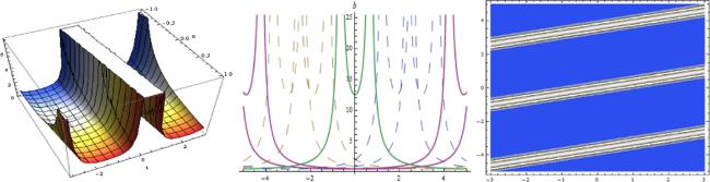
The graphical representation of the SS system is given below by 3D, 2D, and contour plots.
7. Result and discussions
Many authors have worked on the SS diffusion-reaction system. Li et al analyzed the SS diffusion-reaction system for the stability and instability of constant steady-state solutions [51]. Al Noufaey discovered the semi-analytical solutions of the SS system by the Glarekin approach [52]. Iqbal et al explored the soliton solutions of the SS model [42]. Uecker and Wetzel proved the existence of various spatial patterns of the SS system [53]. In this paper, we have utilized LSA to find the infinitesimal generators and symmetries of the SS system represented by equation (1 ). Next, its nonlinear self adjointness has been discussed. Moreover, the sub-ODE method is used to find soliton solutions of the model. Bright and periodic soliton solutions are shown by A1(x, t), B1(x, t), A13(x, t), B13(x, t), A2(x, t), B2(x, t), A5(x, t), B5(x, t), A14(x, t), B14(x, t), A24(x, t), B24(x, t) and A25(x, t), B25(x, t), respectively (figures 1–10). A4(x, t) and B4(x, t) present the dark soliton solutions and their graphical representation is given in figures 4 and 5 and JES solutions are represented by A6(x, t), B6(x, t), A7(x, t), B7(x, t), A8(x, t), B8(x, t), A9(x, t), B9(x, t), A10(x, t), B10(x, t), A11(x, t), B11(x, t), A12(x, t) and B12(x, t) and graphically by figures 8–12. Weierstrass elliptic solutions are presented by A15(x, t), B15(x, t), A16(x, t), B16(x, t), A17(x, t), B17(x, t), A18(x, t) and B18(x, t) and from figures 13–17. Hyperbolic function solutions are given by A22(x, t), B22(x, t) and A23(x, t), B23(x, t) and graphically by figures 18 and 19. The governing model has positive solutions shown by A19(x, t), B19(x, t), A20(x, t), B20(x, t), A21(x, t) and B21(x, t) and graphically by figures 20 and 21.
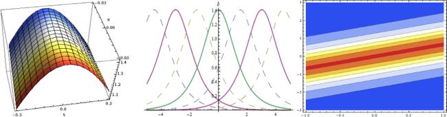
Figure 1. Numerical graphs of solution A1(x, t) for suitable parameters α = 0.5, c = 3, δ = 1, η = 0.5, p = 3, q = 2, Q = − 0.5. |
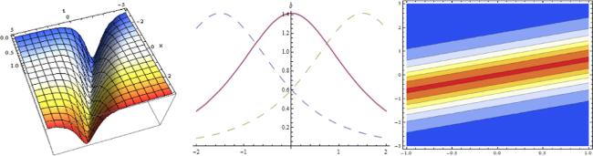
Figure 2. Numerical graphs of solution A2(x, t) for suitable parameters α = 0.5, c = 3, δ = 1, η = 0.5, p = 3, q = 2, Q = 0.5. |
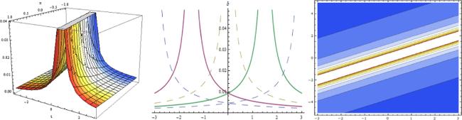
Figure 3. Numerical graphs of solution A3(x, t) for suitable parameters α = 0.5, c = 3, δ = 1, η = − 0.5, p = 3, q = 2, Q = 0.5, ε = 0.01. |
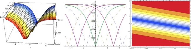
Figure 4. Numerical graphs of solution B4(x, t) for suitable parameters α = 2, c = − 3, δ = 0.5, η = 1, p = 2, q = 2, Q = − 3, ε = 0.01. |
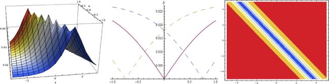
Figure 5. Numerical graphs of solution B5(x, t) for suitable parameters α = 2, c = − 3, δ = 0.5, η = − 2, p = 5, q = 4, Q = 3, ε = 0.01. |
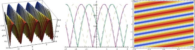
Figure 6. Numerical graphs of solution A7(x, t) for suitable parameters α = 0.5, c = 3, δ = 0, η = 3, m = 1, p = 2, q = 2, Q = 4. |
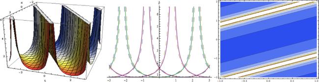
Figure 7. Numerical graphs of solution A10(x, t) for suitable parameters α = − 2, c = 3, δ = 0, η = 3, m = 1, p = 5, q = 2, Q = 0.5. |
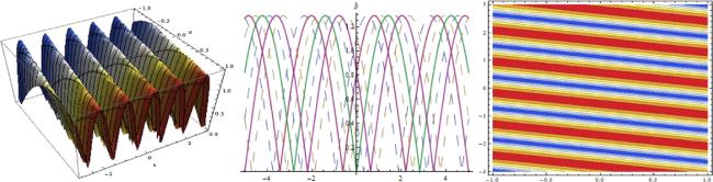
Figure 8. Numerical graphs of solution A12(x, t) for suitable parameters α = 2, c = − 5, δ = 2, η = 3, m = 1, p = 1, q = 2, Q = 0.5. |

Figure 9. Numerical graphs of solution B13(x, t) for suitable parameters α = 2, c = − 1, δ = 0, η = 2, μ = 1, M = − 4, p = 3, q = 2. |
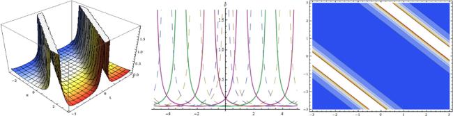
Figure 10. Numerical graphs of solution B14(x, t) for suitable parameters μ = 1, α = 2, c = − 1, δ = 0.5, η = 4, M = 4, p = 3, q = 1. |
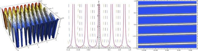
Figure 11. Numerical graphs of solution A15(x, t) for suitable parameters δ = 0.5, α = − 3, β = 2, c = 3, η = 2, H = 1, M = 4, p = 3, q = 2. |
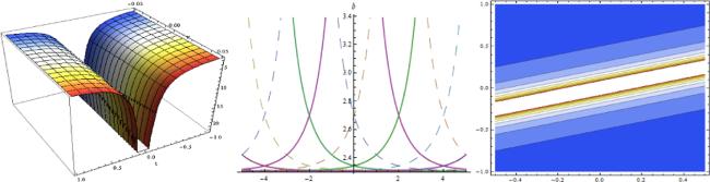
Figure 12. Numerical graphs of solution B16(x, t) for suitable parameters α = − 3, c = 2, δ = 0, η = 2, p = 1, q = 1, Q = 3. |
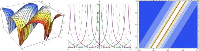
Figure 13. Numerical graphs of solution B17(x, t) for suitable parameters α = − 3, c = 2, δ = 6, η = 2, p = 1, q = 4, Q = 3. |
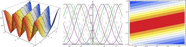
Figure 14. Numerical graphs of solution A18(x, t) for suitable parameters α = 5, c = 2, δ = 1, η = − 2, p = 1, q = 1, Q = 3. |
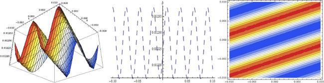
Figure 15. Numerical graphs of solution B19(x, t) for suitable parameters α = 5, c = 25, δ = 15, η = 20, μ = 10, p = 10, q = 10. |
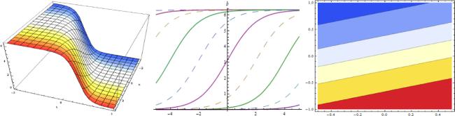
Figure 16. Numerical graphs of solution B20(x, t) for suitable parameters α = 5, c = 2, δ = 1, η = − 4, μ = 2, p = 1, q = 1, Q = 5, ε = 1. |

Figure 17. Numerical graphs of solution B21(x, t) for suitable parameters α = 5c = − 2, δ = 0.25, η = 4, μ = 2, p = 1, q = 1. |
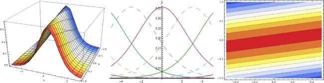
Figure 18. Numerical graphs of solution A22(x, t) for suitable parameters α = 2.5, c = 3, δ = 0, η = 2, μ = 0.5, M = 2, p = 1, q = 1, Q = 1. |
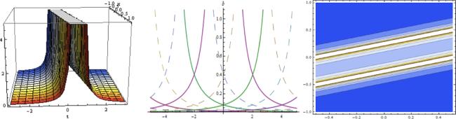
Figure 19. Numerical graphs of solution A23(x, t) for suitable parameters α = 5, c = 2, δ = 0, η = − 4, μ = 1, M = 4, p = 1, q = 1, Q = 1. |
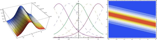
Figure 20. Numerical graphs of solution B24(x, t) for suitable parameters α = − 2.5, c = − 2, δ = 1, η = 2, M = 1, p = 1, q = 1, Q = 2. |
Figure 21. Numerical graphs of solution B25(x, t) for suitable parameters α = − 3, c = 3, δ = 0, η = 3, M = 4, p = 1, q = 1, Q = 2. |
8. Concluding remarks
In this paper, the SS system has been discussed by LSA. We have explored the Lie point symmetries, infinitesimal generators, and the nonlinear SA and CLs of the SS system. Several soliton solutions like bright, dark solitons, periodic solitons, bell, kink shaped, Weierstrass elliptic function solutions, Jacobi, and Hyperbolic are developed for the above model by using the sub-ODE method with the help of Mathematica. A graphical representation is given for all the solutions evaluated in the paper.