


1. Introduction
The study of discrete integrable systems has undergone a true development in the past decades (see [1] and the references therein). One of the key integrability aspects of discrete equations is that of multi-dimensional consistency, which means a lattice equation can be consistently embedded into a higher dimensional system. For quadrilateral lattice equations, such a consistency exhibits the compatibility of these equations is consistent-around-the-cube (CAC) [2–4]. Adler, Bobenko and Suris (ABS) classified all affine linear scalar quadrilateral equations that are CAC with extra conditions (D4 symmetric and tetrahedron property) [5]. The resulting ABS list contains only 9 equations: namely, H1, H2, H3δ, A1δ, A2, Q1δ, Q2, Q3δ and Q4, which are presented in the appendix . In the ABS classification, one scalar quadrilateral equation together with its five copies defined on other five faces compose a consistent cube. An extension of the ABS classification is to allow more than one different equation (e.g. the equations defined on the bottom, left and back sides being different, see figure 2) and their copies to compose a consistent cube [6]. A consistent cube provides useful connections for the involved equations. For example, once we have a consistent cube, the two equations defined on the left side and back side compose a Bäcklund transformation (BT) for the two equations on the bottom and on the top. This point will be explained in detail in the next section. One can also refer to a review paper [7] and the references therein. In [8] various of (non-auto) BTs between different ABS equations were found. Recently, a type of BTs given in [8] was interpreted as a result of deformation of auto BTs of the ABS equations and the torqued versions of the ABS equations were obtained [9]. These torqued ABS equations are not symmetric any longer but integrable in the sense that each of them can compose a consistent cube with known ABS equations. We list these torqued lattice equations together with their corresponding configurations of the consistent cube in the appendix .
The purpose of this paper is to continue to understand the structures of solutions of the torqued ABS equations. Recently we have found that the torqued H2 equation allows a non-autonomous soliton solution [10]. In this paper we will focus on torqued H1 equation (denoted by H1a)appendix ), H1a equation (1 ) is special in the sense that it contains only one spacing parameter p. Since H1 is known as the lattice potential KdV equation, its torqued version, H1a, can be considered as a nonsymmetric discrete KdV equation. We will find solutions for this equation by using BTs generated from the consistent cube. The obtained solutions may provide useful information in understanding torqued lattice equations as nonsymmetric integrable lattice systems.
$\begin{eqnarray}\begin{array}{l}{\rm{H}}{1}^{a}(u,\widetilde{u},\widehat{u},\widehat{\widetilde{u}};p,q)\\ =\,(u-\widetilde{u})(\widehat{\widetilde{u}}-\widehat{u})-p\,=\,0,\end{array}\end{eqnarray}$
and the associated H1 equation $\begin{eqnarray}\begin{array}{l}{\rm{H}}1(u,\widetilde{u},\widehat{u},\widehat{\widetilde{u}};p,q)\\ =\,(u-\widehat{\widetilde{u}})(\widetilde{u}-\widehat{u})-p\,+\,q\,=\,0\end{array}\end{eqnarray}$
and Q1δ equation $\begin{eqnarray}\begin{array}{l}{\rm{Q}}{1}_{0}(u,\widetilde{u},\widehat{u},\widehat{\widetilde{u}};p,q)\\ =p(u-\widehat{u})(\widetilde{u}-\widehat{\widetilde{u}})\\ -q(u-\widetilde{u})(\widehat{u}-\widehat{\widetilde{u}})=0,\end{array}\end{eqnarray}$
which can compose a consistent cube in two ways (see Table A.1). Here, u is a function of $(n,m)\in {{\mathbb{Z}}}^{2}$, p and q serve as spacing parameters in the n-direction and m-direction, respectively, and the involved notations are defined as (see figure 1) $\begin{eqnarray}\begin{array}{l}u\,=\,u(n,m),\,\,\widetilde{u}=u(n+1,m),\\ \widehat{u}=u(n,m+1),\,\,\widehat{\widetilde{u}}=u(n+1,m+1).\end{array}\end{eqnarray}$
Compared with other torqued ABS equations (see Table A.1. Consistency-around-cube of the ABS and torqued ABS equations. |
| Top and Bottom eq | Right and left eq | Back and Front eq |
|---|---|---|
| Q(p, q) = 0 | A(p, r) = 0 | B(r, q) |
| H1a | H1a | H1 |
| H1a | Q10 | H1a |
| H2a | H2a | H2 |
| H2a | Q11 | H2a |
| ${\rm{Q}}{1}_{\delta }^{a}$ | Q1δ | ${\rm{Q}}{1}_{\delta }^{a}$ |
| ${\rm{Q}}{1}_{\delta }^{a}$ | ${\rm{Q}}{1}_{\delta }^{a}$ | Q1δ |
| ${\rm{A}}{1}_{\delta }^{a}$ | ${\rm{A}}{1}_{\delta }^{a}$ | A1δ |
| ${\rm{A}}{1}_{\delta }^{a}$ | Q1δ | ${\rm{A}}{1}_{\delta }^{a}$ |
| Q2a | Q2a | Q2 |
| Q2a | Q2 | Q2a |
| ${\rm{H}}{3}_{0}^{m}$ | ${\rm{H}}{3}_{0}^{m}$ | H30 |
| ${\rm{H}}{3}_{\delta }^{m}$ | ${\rm{H}}{3}_{\delta }^{m}$ | H3δ |
| ${\rm{H}}{3}_{\delta }^{m}$ | ${\rm{Q}}{3}_{0}^{m}$ | ${\rm{H}}{3}_{\delta }^{m}$ |
| A2m | A2m | A2 |
| A2m | Q30 | A2m |
| ${\rm{Q}}{3}_{\delta }^{m}$ | ${\rm{Q}}{3}_{\delta }^{m}$ | ${\rm{Q}}{3}_{\delta }^{m}$ |
| ${\rm{Q}}{3}_{\delta }^{m}$ | ${\rm{Q}}{3}_{\delta }^{m}$ | Q3δ |
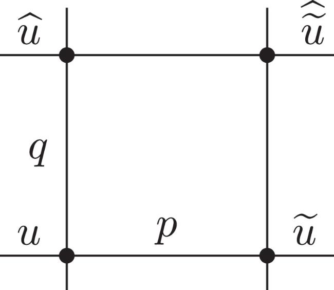
Figure 1. Lattice in ${{\mathbb{Z}}}^{2}$. |
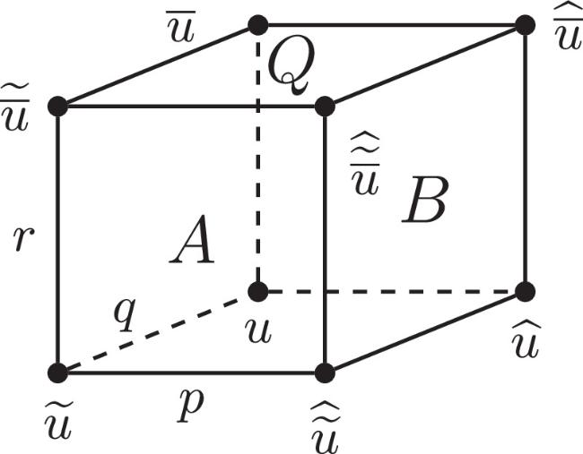
Figure 2. Consistent cube. |
The paper is organized as follows. In section 2 we describe the consistent cubes related to H1a equation, using which we are able to construct its BTs and Lax pairs. In section 3 , we look for solutions using the obtained BTs. Finally, concluding remarks are given in section 4 . There is an appendix where we list ABS equation and torqued ABS equations together with their corresponding configurations of the consistent cube.
2. Consistent cubes and integrability for H1a
CAC is a central notion in the study of discrete integrable systems. For a quadrilateral equation4 ), we denote $\overline{u}=u(n,m,l+1)$ and the spacing parameter of l-direction by r. Suppose there are two more quadrilateral equations
$\begin{eqnarray}Q(u,\widetilde{u},\widehat{u},\widehat{\widetilde{u}};p,q)=0\end{eqnarray}$
defined on the lattice in ${{\mathbb{Z}}}^{2}$ (see figure 1), we extend u from ${{\mathbb{Z}}}^{2}$ to ${{\mathbb{Z}}}^{3}$ and consider u = u(n, m, l) defined on ${{\mathbb{Z}}}^{3}$. Apart from ( $\begin{eqnarray}\begin{array}{l}A(u,\widetilde{u},\overline{u},\widetilde{\overline{u}};p,r)=0,\\ \,\,B(u,\overline{u},\widehat{u},\widehat{\overline{u}};r,q)=0.\end{array}\end{eqnarray}$
The system {Q = 0, A = 0, B = 0}, of which each equation is posed on two opposite faces of a cube (see figure 2 where we have B = 0 on the back and front faces, A = 0 on the left and right faces, and Q = 0 on the bottom and top faces), is called to be CAC if values can be assigned to u and its shifts, such that each equation is satisfied. For multi-linear equations the property is usually characterised as an initial value problem, where $\widehat{\widetilde{\overline{u}}}$ is determined uniquely from $u,\widetilde{u},\widehat{u},\overline{u}$.The equation on the top face reads5 ) rather than a visual shift of u in l-direction, the two side equations in (6 ) compose a BT for equation (5 ). Such an advantage of the CAC property has been used to study lattice equations, such as constructing Lax pairs [3, 11] and generating solutions [10, 12–16].
$\begin{eqnarray}Q(\overline{u},\widetilde{\overline{u}},\widehat{\overline{u}},\widehat{\widetilde{\overline{u}}};p,q)=0.\end{eqnarray}$
Once we have a CAC system and consider $\overline{u}$ as a new solution of equation (There are two CAC systems associated with H1a equation (1 ) [9]. One is
$\begin{eqnarray}\begin{array}{l}Q={\rm{H}}{1}^{a}(u,\widetilde{u},\widehat{u},\widehat{\widetilde{u}};p,q)=0,\\ A={\rm{H}}{1}^{a}(u,\widetilde{u},\overline{u},\widetilde{\overline{u}};p,r)=0,\\ B={\rm{H}}1(u,\overline{u},\widehat{u},\widehat{\overline{u}};r,q)=0.\end{array}\end{eqnarray}$
Another is $\begin{eqnarray}\begin{array}{l}Q={\rm{H}}{1}^{a}(u,\widetilde{u},\widehat{u},\widehat{\widetilde{u}};p,q)=0,\\ A={\rm{Q}}{1}_{0}(u,\widetilde{u},\overline{u},\widetilde{\overline{u}};p,r)=0,\\ B={\rm{H}}{1}^{a}(u,\overline{u},\widehat{u},\widehat{\overline{u}};r,q)=0.\end{array}\end{eqnarray}$
In the first case, the BT reads1 ).
$\begin{eqnarray}\begin{array}{l}A={\rm{H}}{1}^{a}({\rm{p}},{\rm{r}})\\ =\,(u-\widetilde{u})(\widetilde{\overline{u}}-\overline{u})-p\,=\,0,\\ B={\rm{H}}1({\rm{r}},{\rm{q}})\\ =\,(u-\widehat{\overline{u}})(\overline{u}-\widehat{u})-r\,+\,q\,=\,0.\end{array}\end{eqnarray}$
To get a Lax pair, one can introduce $\overline{u}=g/f$ and define Φ = (g, f)T. Then, the above equation gives rise to a linear system $\begin{eqnarray}\widetilde{{\rm{\Phi }}}=L{\rm{\Phi }},\,\,\widehat{{\rm{\Phi }}}=M{\rm{\Phi }},\end{eqnarray}$
where $\begin{eqnarray*}\begin{array}{l}L=\left(\begin{array}{cc}1 & \displaystyle \frac{p}{u-\widetilde{u}}\\ 0 & 1\end{array}\right),\\ M=\left(\begin{array}{cc}u & -(u\widehat{u}+r-q)\\ 1 & -\widehat{u}\end{array}\right).\end{array}\end{eqnarray*}$
The compatibility $\widehat{\widetilde{{\rm{\Phi }}}}=\widehat{\widetilde{{\rm{\Phi }}}}$ leads to a relation $\widehat{L}M=\widetilde{M}L$ which yields the H1a equation (In the second case, the BT is1 ) as well.
$\begin{eqnarray}\begin{array}{l}A={\rm{Q}}{1}_{0}({\rm{p}},{\rm{r}})\,=\\ p(u-\overline{u})(\widetilde{u}-\overline{\widetilde{u}})\\ -r(u-\widetilde{u})(\overline{u}-\overline{\widetilde{u}})=0,\\ B={\rm{H}}{1}^{a}({\rm{r}},{\rm{q}})\\ =\,(u-\overline{u})(\widehat{\overline{u}}-\widehat{u})-r\,=\,0.\end{array}\end{eqnarray}$
Again, introducing $\overline{u}=g/f$ and Φ = (g, f)T, one gets a linear system $\begin{eqnarray}\widetilde{{\rm{\Phi }}}=L{\rm{\Phi }},\,\,\widehat{{\rm{\Phi }}}=M{\rm{\Phi }},\end{eqnarray}$
where now $\begin{eqnarray*}\begin{array}{l}L=\displaystyle \frac{1}{{\left(u-\widetilde{u}\right)}^{2}}\\ \times \left(\begin{array}{cc}{ru}+(p-r)\widetilde{u} & -{pu}\widetilde{u}\\ p & (r-p)u-r\widetilde{u}\end{array}\right),\\ M=\left(\begin{array}{cc}-\widehat{u} & r+u\widehat{u}\\ -1 & u\end{array}\right).\end{array}\end{eqnarray*}$
The compatibility $\widehat{\widetilde{{\rm{\Phi }}}}=\widehat{\widetilde{{\rm{\Phi }}}}$ leads to $\widehat{L}M=\widetilde{M}L$, that is $\begin{eqnarray*}\begin{array}{l}\widehat{L}M-\widetilde{M}L\,=\\ \left(\begin{array}{cc}\displaystyle \frac{-p\,-\,(u\,-\,\widetilde{u})(\widehat{u}\,-\,\widehat{\widetilde{u}})}{u\,-\,\widetilde{u}} & \displaystyle \frac{(p+(u\,-\,\widetilde{u})(\widehat{u}\,-\,\widehat{\widetilde{u}}))(u\widehat{u}\,-\,\widetilde{u}\widehat{\widetilde{u}})}{(u\,-\,\widetilde{u})(\widehat{u}\,-\,\widehat{\widetilde{u}})}\\ 0 & u\,-\,\widetilde{u}+\displaystyle \frac{p}{\widehat{u}\,-\,\widehat{\widetilde{u}}}\end{array}\right)=0,\end{array}\end{eqnarray*}$
which gives rise to H1a equation (In the next section, we will focus on BTs to construct soliton solutions.
3. Solutions for H1a
To get a soliton solution using BT (e.g.[15]), one needs to have a seed solution first. Obviously, the H1a equation (1 ) has a simple solution u0 = an + γ where p = − a2 and γ is an arbitrary constant.
It can be verified that for the arbitrary function $w=w(m)$ that is independent of n,
$\begin{eqnarray}u={an}+\gamma +w(m)\end{eqnarray}$
is always a solution to the ${\rm{H}}{1}^{a}$ equation (In the following we shall look for solutions different from the above type.
3.1. Solutions from BT (10 )
Consider BT (10 ) where r acts as a BT parameter. Seed solution can be found using the ‘fixed point’ idea [15], that is, assuming BT parameter r does not make sense in generating new solution $\overline{u}$, and in practice, setting $\overline{u}=u$ in a BT.
Taking $\overline{u}=u$ in (10 ) we get15 ) indicates1 ).
$\begin{eqnarray}{\left(u-\widetilde{u}\right)}^{2}={a}^{2},\,\,{\left(u-\widehat{u}\right)}^{2}={b}^{2},\end{eqnarray}$
where we have taken r = c and parameterized $\begin{eqnarray}p=-{a}^{2},\quad q-c=-{b}^{2}.\end{eqnarray}$
Equation ( $\begin{eqnarray}u={an}+{bm}+\gamma ,\end{eqnarray}$
where γ is a constant, which can be verified to be a solution of the H1a equation (Corresponding the parametrisation (16 ), we look for a new solution $\overline{u}$ from the BT (10 ), i.e.16 ), and the seed solution u that we use is (17 ). We look for $\overline{u}$ in the following form (cf.[15])18 ). It follows that19 ) falls into the form (14 ) and the solution (19 ) is at most a special case of (14 ). Therefore we stop the proceeding of this case and turn to considering another BT.
$\begin{eqnarray}\begin{array}{l}(u-\widetilde{u})(\widetilde{\overline{u}}-\overline{u})=-{a}^{2},\\ (u-\widehat{\overline{u}})(\overline{u}-\widehat{u})={b}^{2}-{k}^{2},\end{array}\end{eqnarray}$
where we have taken r = c − k2, as b for q in ( $\begin{eqnarray}\overline{u}={an}+{bm}+k+\gamma +v\end{eqnarray}$
and determine v from ( $\begin{eqnarray}\begin{array}{l}\widetilde{v}=v,\,\,\widehat{v}=\displaystyle \frac{{Av}}{B\,+\,v},\\ A=-(b+k),\,\,B=-(b-k),\end{array}\end{eqnarray}$
which indicates that v is a function independent of n from $\widetilde{v}=v$. Thus, (3.2. Solutions from BT (12 )
We can try the fixed point idea on BT (12 ) but the setting $\overline{u}=u$ does not generate any solutions. Noticing that the H1a equation (1 ) is invariant in the transformation u → u + c with any constant c, we consider the setting $\overline{u}=u+c$ in BT (12 ) and it gives rise to17 ) can be a solution resulting from (21 ) with parametrisation
$\begin{eqnarray}r{\left(u-\widetilde{u}\right)}^{2}={{pc}}^{2},\,\,-{c}^{2}=r.\end{eqnarray}$
This indicates that ( $\begin{eqnarray}p=-{a}^{2},\,\,r=-{c}^{2},\end{eqnarray}$
and we have included the term bm without loss of generality.To get one-soliton solution, we now consider the BT (12 ) with parametrisation p = − a2 and r = − k2 where k serves as the BT number, which reads17 ) as a seed solution and $\overline{u}$ takes a form14 ) because now v evolves with n.
$\begin{eqnarray}\begin{array}{l}{a}^{2}(u-\overline{u})(\widetilde{u}-\widetilde{\overline{u}})\\ -{k}^{2}(u-\widetilde{u})(\overline{u}-\widetilde{\overline{u}})=0,\\ (u-\overline{u})(\widehat{\overline{u}}-\widehat{u})=-{k}^{2}.\end{array}\end{eqnarray}$
We assume in the above BT u is given as ( $\begin{eqnarray}\overline{u}={an}+{bm}+k+\gamma +v\end{eqnarray}$
and we look for v. It turns out that v satisfies $\begin{eqnarray*}\begin{array}{l}\widetilde{v}=\displaystyle \frac{{Av}}{B+{av}},\,\,\widehat{v}=\displaystyle \frac{-{kv}}{k+v},\\ A=-k(a+k),\,\,B=k(a-k).\end{array}\end{eqnarray*}$
To solve it out, we introduce $v=\tfrac{f}{g}$ and Φ = (f, g)T, which lead us to a linear system $\begin{eqnarray*}\begin{array}{l}\widetilde{{\rm{\Phi }}}={ \mathcal N }{\rm{\Phi }},\\ \quad \widehat{{\rm{\Phi }}}={ \mathcal M }{\rm{\Phi }},\end{array}\end{eqnarray*}$
where $\begin{eqnarray*}\begin{array}{l}{ \mathcal N }=\left(\begin{array}{cc}A & 0\\ a & B\end{array}\right),\quad \quad { \mathcal M }=\left(\begin{array}{cc}-k & 0\\ 1 & k\end{array}\right).\end{array}\end{eqnarray*}$
After some calculation, we arrive at $\begin{eqnarray*}\begin{array}{l}{f}_{n,m}={\left(-k\right)}^{n+m}{\left(a+k\right)}^{n}{f}_{\mathrm{0,0}},\\ {g}_{n,m}=-\displaystyle \frac{{k}^{n+m-1}}{2}{f}_{\mathrm{0,0}}{\left(-1\right)}^{m+n}{\left(a+k\right)}^{n}\\ +\displaystyle \frac{{k}^{n+m-1}}{2}{f}_{\mathrm{0,0}}{\left(a-k\right)}^{n}\\ +{k}^{n+m}{\left(a-k\right)}^{n}{g}_{\mathrm{0,0}},\end{array}\end{eqnarray*}$
where f0,0 and g0,0 are constants. Therefore $\begin{eqnarray*}\begin{array}{l}{v}_{n,m}=\displaystyle \frac{{f}_{n,m}}{{g}_{n,m}}\,=\\ \displaystyle \frac{{\left(-k\right)}^{n+m}{\left(a+k\right)}^{n}{f}_{\mathrm{0,0}}}{-\tfrac{{k}^{n+m-1}}{2}{f}_{\mathrm{0,0}}{\left(-1\right)}^{m+n}{\left(a+k\right)}^{n}+\tfrac{{k}^{n+m-1}}{2}{f}_{\mathrm{0,0}}{\left(a-k\right)}^{n}+{k}^{n+m}{\left(a-k\right)}^{n}{g}_{\mathrm{0,0}}},\end{array}\end{eqnarray*}$
which can be written in a neat form $\begin{eqnarray}{v}_{n,m}=\displaystyle \frac{-2k{\rho }_{n,m}}{1+{\rho }_{n,m}},\end{eqnarray}$
where $\begin{eqnarray}{\rho }_{n,m}={\left(\displaystyle \frac{k+a}{k-a}\right)}^{n}{\left(-1\right)}^{m}{\rho }_{\mathrm{0,0}}\end{eqnarray}$
is called plane wave factor (PWF) and ρ0,0 is a constant. Thus, the 1-soliton solution can be given by $\begin{eqnarray}\begin{array}{l}{u}_{1{ss}}={an}+{bm}+\gamma +\\ \displaystyle \frac{k(1-{\rho }_{n,m})}{1+{\rho }_{n,m}}.\end{array}\end{eqnarray}$
Apparently, this is a solution that is different from the type of (For multi-soliton solutions, let us define $\psi (n,m;l)={\left({\psi }_{1},{\psi }_{2},\cdots ,{\psi }_{N}\right)}^{{\rm{T}}}$ where
$\begin{eqnarray}\begin{array}{l}{\psi }_{i}(n,m;l)={\varrho }_{i}^{+}{k}_{i}^{l}{k}_{i}^{m}{\left({k}_{i}+a\right)}^{n}\\ +{\varrho }_{i}^{-}{\left(-{k}_{i}\right)}^{l}{\left(-{k}_{i}\right)}^{m}{\left({k}_{i}-a\right)}^{n}\end{array}\end{eqnarray}$
with constants ${\varrho }_{i}^{\pm }$ and ki, and define $\begin{eqnarray*}\begin{array}{l}f=\left|\psi (l),\psi (l+1),\cdots ,\right.\\ \left.\psi (l+N-1)\right|\equiv \left|\widehat{N-1}\right|,\\ g=\left|\psi (l),\psi (l+1),\cdots ,\right.\\ \left.\psi (l+N-2),\psi (l+N)\right|\\ \equiv \left|\widehat{N-2},N\right|.\end{array}\end{eqnarray*}$
Then, it can be verified that the ${\rm{H}}{1}^{a}$ equation ( $\begin{eqnarray}{uNss}={an}+{bm}+\gamma -\displaystyle \frac{g}{f}\end{eqnarray}$
for N = 2, 3. We are left to prove for all N. For H1 equation (
$\begin{eqnarray}\begin{array}{l}{\rho }_{n,m}={\left(\displaystyle \frac{a+k}{a-k}\right)}^{n}\\ \times {\left(\displaystyle \frac{b+k}{b-k}\right)}^{m}{\rho }_{\mathrm{0,0}}.\end{array}\end{eqnarray}$
There is the systematic Cauchy matrix approach [17, 18] to generate integrable lattice equations starting from the above PWF. It would be interesting to develop the Cauchy matrix approach for non-symmetric lattice equations.4. Concluding remarks
In this paper, we have presented Lax pairs and some solutions for the torqued H1 equation, namely H1a. Since H1 is known as the lattice potential KdV equation, one can consider H1a as a nonsymmetric version of the discrete KdV equation. This equation is special in the torqued ABS equations because among those equations it is the only equation that contains a single spacing parameter. We derived its Lax pairs using BTs constructed from the consistent cubes. The first BT leads to a solution whose principle part (after removing the linear background) depends only on m, which belongs to the more general form described in Remark 1 . The second BT does contribute a solution (27 ) that involves both directions in the PWF (26 ).
H1 equation (2 ) is the simplest equation in the ABS list and it usually serves as a model equation in the research of discrete integrable systems. As we have mentioned in Remark 3 , we hope the research we have done on H1a can provide useful information in understanding torqued lattice equations and their continuous counterparts, as well as in developing research means such as the Cauchy matrix approach and bilinear method for nonsymmetric integrable lattice systems.
Appendix. ABS and torqued ABS equations and consistency cube
The ABS equations are [5]
$\begin{eqnarray*}\begin{array}{l}{\rm{H}}1:\quad (u-\widehat{\widetilde{u}})(\widetilde{u}-\widehat{u})\\ -p+q=0,\\ {\rm{H}}2:\quad (u-\widehat{\widetilde{u}})(\widetilde{u}-\widehat{u})\\ -(p-q)(u+\widetilde{u}+\widehat{u}+\\ \widehat{\widetilde{u}}+p+q)=0,\\ {\rm{H}}{3}_{\delta }:\quad {\rm{p}}(u\widetilde{u}+\widehat{u}\widehat{\widetilde{u}})\\ -q(u\widehat{u}+\widetilde{u}\widehat{\widetilde{u}})+\delta ({p}^{2}-{q}^{2})=0,\\ {\rm{A}}{1}_{\delta }:\quad {\rm{p}}(u+\widehat{u})(\widetilde{u}+\widehat{\widetilde{u}})\\ -q(u+\widetilde{u})(\widehat{u}+\widehat{\widetilde{u}})\\ -{\delta }^{2}{pq}(p-q)=0,\\ {\rm{A}}2:\quad {\rm{p}}(1-{{\rm{q}}}^{2})(u\widetilde{u}+\widehat{u}\widehat{\widetilde{u}})\\ -q(1-{p}^{2})(u\widehat{u}+\widetilde{u}\widehat{\widetilde{u}})\\ -({p}^{2}-{q}^{2})(1+u\widetilde{u}\widehat{u}\widehat{\widetilde{u}})=0,\\ {\rm{Q}}{1}_{\delta }:\quad {\rm{p}}(u-\widehat{u})(\widetilde{u}-\widehat{\widetilde{u}})\\ -q(u-\widetilde{u})(\widehat{u}-\widehat{\widetilde{u}})\\ +{\delta }^{2}{pq}(p-q)=0,\\ {\rm{Q}}2:\quad {\rm{p}}(u-\widehat{u})(\widetilde{u}-\widehat{\widetilde{u}})\\ -q(u-\widetilde{u})(\widehat{u}-\widehat{\widetilde{u}})\\ +{pq}(p-q)(u+\widetilde{u}+\widehat{u}+\widehat{\widetilde{u}}-{p}^{2}+{pq}-{q}^{2})=0,\\ {\rm{Q}}{3}_{\delta }:\quad {\rm{p}}(1-{{\rm{q}}}^{2})(u\widehat{u}+\widetilde{u}\widehat{\widetilde{u}})\\ -q(1-{p}^{2})(u\widetilde{u}+\widehat{u}\widehat{\widetilde{u}})\\ -({p}^{2}-{q}^{2})\left(\widetilde{u}\widehat{u}+u\widehat{\widetilde{u}}\right.\\ \left.+\displaystyle \frac{{\delta }^{2}(1-{p}^{2})(1-{q}^{2})}{4{pq}}\right)=0,\\ {\rm{Q}}4:\quad \mathrm{sn}({\rm{p}})(u\widetilde{u}+\widehat{u}\widehat{\widetilde{u}})\\ -\mathrm{sn}(q)(u\widehat{u}+\widetilde{u}\widehat{\widetilde{u}})\\ +\mathrm{sn}(p-q)\left(k\,\mathrm{sn}(p)\mathrm{sn}(q)(u\widetilde{u}\widehat{u}\widehat{\widetilde{u}}+1)\right.\\ \left.-\widetilde{u}\widehat{u}-u\widehat{\widetilde{u}}\right)=0,\end{array}\end{eqnarray*}$
where the present form of Q4 is due to [19] and and sn is the Jacobi elliptic function of modulus k. The corresponding torqued ABS equations are [9] $\begin{eqnarray*}\begin{array}{l}{\rm{H}}{1}^{a}:\quad (u-\widetilde{u})(\widehat{\widetilde{u}}-\widehat{u})-{\rm{p}}=0,\\ {\rm{H}}{2}^{a}:\quad (u-\widetilde{u})(\widehat{\widetilde{u}}-\widehat{u})\\ -p(u+\widetilde{u}+\widehat{u}+\widehat{\widetilde{u}}+p+2q)=0,\\ {\rm{H}}{3}_{\delta }^{m}:\quad {\rm{p}}(u\widehat{\widetilde{u}}+\widehat{u}\widetilde{u})\\ -(u\widehat{u}+\widetilde{u}\widehat{\widetilde{u}})\\ +\delta ({p}^{2}-1)q=0,\\ {\rm{A}}{1}_{\delta }^{a}:\quad ({\rm{p}}+{\rm{q}})(u+\widehat{u})(\widetilde{u}+\widehat{\widetilde{u}})\\ -q(u+\widehat{\widetilde{u}})(\widehat{u}+\widetilde{u})\\ -{\delta }^{2}{pq}(p+q)=0,\\ {\rm{A}}{2}^{m}:\quad {\rm{p}}(1-{{\rm{q}}}^{2})(u\widehat{\widetilde{u}}+\widehat{u}\widetilde{u})\\ -(1-{p}^{2}{q}^{2})(u\widehat{u}+\widetilde{u}\widehat{\widetilde{u}})\\ -({p}^{2}-1)q(1+u\widetilde{u}\widehat{u}\widehat{\widetilde{u}})=0,\\ {\rm{Q}}{1}_{\delta }^{a}:\quad ({\rm{p}}+{\rm{q}})(u-\widehat{u})(\widehat{\widetilde{u}}-\widetilde{u})\\ -q(u-\widehat{\widetilde{u}})(\widehat{u}-\widetilde{u})\\ +{\delta }^{2}{pq}(p+q)=0,\\ {\rm{Q}}{2}^{a}:\quad ({\rm{p}}+{\rm{q}})(u-\widehat{u})(\widehat{\widetilde{u}}-\widetilde{u})\\ -q(u-\widehat{\widetilde{u}})(\widehat{u}-\widetilde{u})\\ +{pq}(p+q)(u+\widetilde{u}+\widehat{u}+\widehat{\widetilde{u}}-{p}^{2}-{pq}-{q}^{2})=0,\\ {\rm{Q}}{3}_{\delta }^{m}:\quad {\rm{p}}(1-{{\rm{q}}}^{2})(u\widehat{u}+\widetilde{u}\widehat{\widetilde{u}})\\ -(1-{p}^{2}{q}^{2})(u\widehat{\widetilde{u}}+\widehat{u}\widetilde{u})\\ \,\,\,\,-({p}^{2}-1)q\left(u\widetilde{u}+\widehat{u}\widehat{\widetilde{u}}+\displaystyle \frac{{\delta }^{2}(1-{p}^{2}{q}^{2})(1-{q}^{2})}{4{{pq}}^{2}}\right)=0,\\ {\rm{Q}}{4}^{a}:\quad \mathrm{sn}({\rm{p}}+{\rm{q}})(u\widehat{\widetilde{u}}+\widehat{u}\widetilde{u})\\ -\mathrm{sn}(q)(u\widehat{u}+\widetilde{u}\widehat{\widetilde{u}})\\ +\mathrm{sn}(p)\\ \times \left(k\,\mathrm{sn}(p+q)\mathrm{sn}(q)(u\widetilde{u}\widehat{u}\widehat{\widetilde{u}}+1)-\widehat{\widetilde{u}}\widehat{u}-u\widetilde{u}\right)=0.\end{array}\end{eqnarray*}$