


1. Introduction
Partial differential equations (PDEs) are widely used to describe nonlinear phenomena in nature [1–3]. And, solving PDEs is helpful in understanding the physical laws behind these nonlinear phenomena [4–7]. However, analytical solutions of PDEs are often very difficult to obtain [8]. Accordingly, numerical methods have been proposed and promoted the study of PDEs [9, 10]. Due to the large computational demands of these methods, the accuracy and efficiency of solving PDEs are difficult to acquire simultaneously.
In recent years, deep learning methods have been extended from natural language recognition and machine translation to scientific computing, and have provided new ideas for solving PDEs [11–13]. According to the universal approximation theorem, a multilayered feed forward network containing a sufficient number of hidden neurons can approximate any continuous function with arbitrary accuracy [14, 15], which provides the theoretical support for deep learning to solve PDEs. At this stage, there are two types of deep learning methods for solving PDEs [16]. The first type keep the same learning approach as the original deep learning methods. The basic theory is constructing neural operators by learning mappings from function parameter dependence to solutions, such as Deeponet, Fourier neural operator, so on [17, 18]. This type needs to be trained only once to handle different initial value problems, but requires a large amount of data with high fidelity. The second type combines deep learning with physical laws. In second type, the physical laws and a small amount the initial and boundary data of PDEs are used to constrain the network training instead of lots of labeled data. The representative is physics informed neural networks (PINNs) that can solve both nonlinear PDEs and corresponding inverse problems [19]. Based on the original PINNs, many improved versions were proposed [20–26]. Ameya et al set a scalable hyper-parameter in the activation function and proposed an adaptive activation function with better learning capabilities and convergence speed [22]. Lin and Chen devise a two-stage PINNs method based on conserved quantities, which better exploits the properties of PDEs [23]. In addition to the physical laws, the variational residual of PDEs is also considered as a loss term, such as deep Ritz method, deep Galerkin method and so on [27–29]. As the intensive study of the PINNs and its variants, these algorithms are applied to many fields, such as biomedical problems [30], continuum micromechanics [31], stiff chemical kinetics [32]. Inspired by the PINNs, some deep learning solver for non-fully connected structures are proposed. Zhu et al constructed a physics-constrained convolutional encoding-decoding structure for stochastic PDEs [33]. Based on the work of Zhu et al, physics-informed convolutional-recurrent networks combined with long short-term memory network (LSTM) were proposed, while the initial and boundary conditions were hard-encoded into the network [34]. Mohan et al used an extended convolutional LSTM to model turbulence [35]. Based on this, Stevens et al exploited the temporal structure [36]. In general, existing deep learning solvers with LSTM structures can approximate the dynamic behavior of the solution without any labeled data, but the implementations rely on feature extraction of convolutional structures and are complex.
The aim of this paper is to build a flexible deep learning solver based on physical laws and temporal structures. Therefore, physics informed memory networks (PIMNs) based on LSTM framework is proposed as a new method for solving PDEs. In the PIMNs, the differential operator is approximated using difference schemes rather than automatic differentiation (AD). AD is flexible and ingenious, but loses information about the neighbors of the sampling points [37]. The differential schemes are implemented as convolution filter, and the convolution filter is only used to calculate the physical residuals and does not change with network training. This is different from existing solvers with convolutional structures. Numerical experiments on the KdV equation and the nonlinear Schrödinger equation show that the PIMNs can achieve excellent accuracy and are insensitive to the boundary conditions.
The rest of the paper is organized as follows. In section 2 , the general principle and network architectures of the PIMNs are elaborated. In section 3 , two sets of numerical experiments are given and the effects of various influencing factors on the learned solution are discussed. Conclusion is given in last section.
2. Physics informed memory networks
2.1. Problem setup
In general, the form of PDEs that can be solved by physical informed deep learning is as follows:
$\begin{eqnarray}\begin{array}{rcl}{u}_{t}+{ \mathcal N }[u] & = & 0,x\in [{x}_{0},{x}_{1}],t\in [0,T],\\ u(x,0) & = & {u}_{0}(x),\\ u({x}_{0},t) & = & {u}_{1}(t),\\ u({x}_{1},t) & = & {u}_{2}(t),\end{array}\end{eqnarray}$
where u(x, t) is the solution of PDEs and ${ \mathcal N }[u]$ is a nonlinear differential operator. u0(x) and u1(t), u2(t) are initial and boundary functions, respectively. And, the basic theory of physical informed deep learning is approximating the solution u(x, t) through the constraints of the physical laws [15]. Therefore, the PDEs residual f(x, t) is defined as $\begin{eqnarray}f(x,t):= {u}_{t}+{ \mathcal N }[u].\end{eqnarray}$
The keys of the PIMNs are the calculation of physical residuals f(x, t) using the difference schemes and the establishment of the corresponding long-term dependence.2.2. Physics informed memory networks
The structure of the LSTM unit is shown in figure 1. Xt, ht, ct, $\tilde{{c}_{t}}$, ft, it, ot are the input, the hidden state, the cell state, the internal cell state, the forget gate, the input gate, the output gate, respectively. ft and it control the information forgotten and added to ct. $\tilde{{c}_{t}}$ is the information added to ct. The output is determined jointly by ot and ct. The mathematical expression of LSTM is shown as follows:
$\begin{eqnarray}\begin{array}{rcl}{f}_{t} & = & \sigma \left({W}_{{Xf}}{X}_{t}+{W}_{{hf}}{h}_{t-1}+{b}_{f}\right),\\ {i}_{t} & = & \sigma \left({W}_{{Xi}}{X}_{t}+{W}_{{hi}}{h}_{t-1}+{b}_{i}\right),\\ \tilde{{c}_{t}} & = & \tanh \left({W}_{{Xc}}{X}_{t}+{W}_{{hc}}{h}_{t-1}+{b}_{c}\right),\\ {c}_{t} & = & {f}_{t}\circ {c}_{t-1}+{i}_{t}\circ \tilde{{c}_{t}},\\ {o}_{t} & = & \sigma \left({W}_{{Xo}}{X}_{t}+{W}_{{ho}}{h}_{t-1}+{W}_{{co}}\circ {c}_{t}+{b}_{o}\right),\\ {h}_{t} & = & {o}_{t}\circ \tanh \left({c}_{t}\right).\end{array}\end{eqnarray}$
Here, W, b are the network parameters, and ◦ represents the Hadamard product.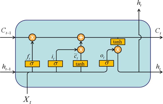
Figure 1. The general structure of LSTM. |
In the PIMNs, subscripts and superscripts of hti and cti refer to the number of time series and layers, respectively. LSTM unit imports the output hti of the current moment t to the next moment t + 1, which links all moments of the same spatial point. In addition, hti is also used as input to moment t for the next LSTM layer, which strengthens the connection between different moments. It should be noted that the hidden nodes of the last LSTM are fixed. In fact, we use the last LSTM to control the dimensionality of the output.
As shown in figure 2, the inputs to the PIMNs are the coordinates of the grid points in the region [x0, x1] × [0, T]. The region [x0, x1] × [0, T] is meshed into (m + 1) × (n + 1) grid points. Each set of inputs to the PIMNs are coordinate values (xi, t0), (xi, t1), ⋯,(xi, tn) at the same location. The outputs are the corresponding ${u}_{0}^{i},{u}_{1}^{i},\cdots ,{u}_{n}^{i}$ (corresponding to each row of the left panel of figure 3). Based on the output uij of the PIMNs, their loss functions can be constructed. The loss function of includes three components:2 ). MSEf, MSEI and MSEB correspond to the physical residuals, initial and boundary losses, respectively. MSEI and MSEB are obtained by the learned solution and the corresponding known data. The terms ut, ux, etc for constructing MSEf are obtained from the difference schemes and are computed as (in the case of the second-order center difference):
$\begin{eqnarray}\mathrm{MSE}={\mathrm{MSE}}_{f}+{\mathrm{MSE}}_{I}+{\mathrm{MSE}}_{B},\end{eqnarray}$
where $\begin{eqnarray}{\mathrm{MSE}}_{f}=\frac{1}{(m+1)(n+1)}\sum _{i=1}^{m+1}\sum _{j=1}^{n+1}| {f}_{j}^{i}{| }^{2},\end{eqnarray}$
$\begin{eqnarray}{\mathrm{MSE}}_{I}=\frac{1}{m+1}\sum _{i=1}^{m+1}| {u}_{0}^{i}-u({x}_{i},{t}_{0}){| }^{2},\end{eqnarray}$
$\begin{eqnarray}\begin{array}{ccc}{\mathrm{MSE}}_{B} & = & \frac{1}{n+1}\displaystyle \sum _{j=1}^{n+1}| {u}_{j}^{0}-u({x}_{0},{t}_{j}){| }^{2}\\ & & +\frac{1}{n+1}\displaystyle \sum _{j=1}^{n+1}| {u}_{j}^{m}-u({x}_{m},{t}_{j}){| }^{2}.\end{array}\end{eqnarray}$
Here, uji and u(xi, tj) are the numerical solution and exact solution for the grid points (xi, tj), respectively. fji is the physical residual for the grid points (xi, tj). uji is the output of the PIMNs and fji is obtained by taking the terms ut, ux, etc, constructed based on uji into equation ( $\begin{eqnarray}{u}_{j,x}^{i}=\displaystyle \frac{{u}_{j}^{i+1}-{u}_{j}^{i-1}}{2\delta x},\end{eqnarray}$
$\begin{eqnarray}{u}_{j,t}^{i}=\displaystyle \frac{{u}_{j+1}^{i}-{u}_{j-1}^{i}}{2\delta t}.\end{eqnarray}$
Here, δx and δt represent spatial and temporal intervals, respectively. To accelerate the training, the difference schemes are implemented by convolution operations. Taking second-order central difference schemes as an example, the convolution filters are: $\begin{eqnarray}{K}_{x}={\left[-\mathrm{1,0,1}\right]}^{T}\times \displaystyle \frac{1}{2\delta x},\end{eqnarray}$
$\begin{eqnarray}{K}_{t}=[-1,0,1]\times \displaystyle \frac{1}{2\delta t}.\end{eqnarray}$
Figure 3 illustrates the computation of ux and ut. Higher order derivatives can be obtained by performing a difference operation on ux and ut, such as $\begin{eqnarray}{u}_{j,{xx}}^{i}=\displaystyle \frac{{u}_{j,x}^{i+1}-{u}_{j,x}^{i-1}}{2\delta x}.\end{eqnarray}$
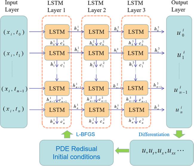
Figure 2. The general structure of the PIMNs. |
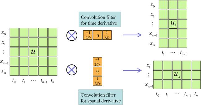
Figure 3. The convolution process of difference schemes. |
As shown in figure 3, the padding is not done to avoid unnecessary errors. This leads to the fact that ut at t = t0, t = tn and ux at x = x0, x = xm cannot be computed (in terms of the second-order central difference). In other words, fj i cannot be computed at t = t0 (i.e. the initial condition) due to the lack of ${u}_{-1}^{i}$. A similar problem arises with the boundary conditions. Therefore, fj i at t = t0, x = x0 and x = xm will not be used to compute the loss. When higher order derivative terms are included in fj i, the region in which losses are not computed is correspondingly enlarged. In fact, since the spatial and temporal intervals we obtain are usually small and the boundaries of the domain can be bounded by the initial and boundary conditions, the numerical solutions of the PDEs can be approximated even without computing fj i near the boundaries of the domain. And, the boundary conditions are not necessary, which will be tested in the numerical experiments. Correspondingly, the total loss excludes the boundary loss when the boundary condition is missing. In addition, the spatial derivatives at t0 are constructed by known initial conditions. Therefore, except for being the target for the initial loss, the initial conditions are also used indirectly for the PDEs residuals.
3. Numerical experiments
In this section, the PIMNs are applied to solve the KdV equation and the nonlinear Schrödinger equation. Specifically, the effects of different difference schemes on the solving ability of the PIMNs are discussed, and the network structure and mesh size that minimize the error are investigated. Moreover, the performance of the PIMNs and the PINNs are compared.
In the numerical experiments, the implementation of the PIMNs is based on Python 3.7 and Tensorflow 1.15. The loss function is chosen as the mean squared loss function, and L-BFGS is used to optimize the loss function. All numerical examples reported here are run on a Lenovo Y7000P 2020H computer with 2.60 GHz 6-core Intel(R) Core(TM) i7-10750H CPU and 16 GB memory. In addition, the relative L2 error is used to measure the difference between the predicted and true values and is calculated as follows:
$\begin{eqnarray}{\mathrm{Error}}_{{L}_{2}}=\frac{{\sum }_{i=1}^{m+1}{\sum }_{j=1}^{n+1}| {u}_{j}^{i}-u({x}_{i},{t}_{j}){| }^{2}}{{\sum }_{i=1}^{m+1}{\sum }_{j=1}^{n+1}| u({x}_{i},{t}_{j}){| }^{2}}.\end{eqnarray}$
Here, uji and u(xi, tj) are the numerical solution and exact solution for the grid points (xi, tj), respectively. Thus, the relative L2 error is obtained by calculating the numerical and exact solutions for all grid points.3.1. Case 1: The KdV equation
The KdV equation is a classical governing model for the propagation of shallow water waves and has important applications in many areas of physics, such as fluid dynamics, plasma [39–41]. In general, the KdV equation is given by14 ) can be referred to in the [42]. Here, the traveling wave solution is simulated:16 ) is reduced to
$\begin{eqnarray}\begin{array}{rcl}{q}_{t}+6{{qq}}_{x}+{q}_{{xxx}} & = & 0,x\in [{x}_{0},{x}_{1}],t\in [{t}_{0},{t}_{1}],\\ q(x,{t}_{0}) & = & {q}_{0}(x),\\ q({x}_{0},t) & = & {q}_{1}(x),\\ q({x}_{1},t) & = & {q}_{2}(x),\end{array}\end{eqnarray}$
where q0(x) is an initial function, and q1(x) and q2(x) are boundary functions. x0 and x1 are arbitrary real constants. The PDEs residual f(x, t) corresponding to the KdV equation is: $\begin{eqnarray}f(x,t):= {q}_{t}+6{{qq}}_{x}+{q}_{{xxx}}.\end{eqnarray}$
And, the existence theory of equation ( $\begin{eqnarray}q(x,t)=a+2{k}^{2}{{\rm{sech}} }^{2}\left\{k[x-(4{k}^{2}+6{u}_{0})t+{x}_{0}]\right\},\end{eqnarray}$
where ${k}^{2}=\tfrac{1}{2}(c-a)$, a, c are real constants and c > a. Taking a = 0.1, c = 0.8, x0 = 0, equation ( $\begin{eqnarray}q(x,t)=0.1+0.7{{\rm{sech}} }^{2}\left[\displaystyle \frac{\sqrt{7}}{2\sqrt{5}}(x-2t)\right].\end{eqnarray}$
Taking [x0, x1] and [t0, t1] as [−10, 10] and [0, 1], the corresponding initial and boundary functions are obtained.3.1.1. Comparison of different difference schemes for solving the KdV equation
In section 2.2 , we constructed the PDEs residuals by the second-order central difference. However, it is important to discuss which difference scheme is suitable for constructing time derivatives for establishing the long-term dependence of PDEs. Here, forward difference, backward difference and central difference are used to computer the temporal derivatives, respectively. The space [−10, 10] is divided into 1000 points and the time [0, 1] is divided into 100 points. Two LSTM layers are used with the number of nodes 30 and 1, respectively. Since the initialization of the network parameters is based on random number seeds, 4 sets of experiments based on different random number seeds (i.e. 1, 2, 3, 4 in table 1) were set up in order to avoid the influence of chance. The relative errors for four sets of numerical experiments are given in table 1.
Table 1. The KdV equation: relative L2 errors for different difference schemes. |
| Difference schemes | Forward difference | Backward difference | Central difference |
|---|---|---|---|
| 1 | 4.355 988 × 10−3 | 4.638 906 × 10−3 | 2.034 928 × 10−3 |
| 2 | 4.058 963 × 10−3 | 4.640 369 × 10−3 | 1.317 186 × 10−3 |
| 3 | 4.884 505 × 10−3 | 4.459 566 × 10−3 | 1.124 485 × 10−3 |
| 4 | 4.580 123 × 10−3 | 4.348 073 × 10−3 | 9.399 773 × 10−4 |
From the data in table 1, the PIMNs can solve the KdV equation with very high accuracy for all three difference methods. The bolded data are the lowest relative L2 errors produced by the same random number. It can be clearly seen that the relative L2 errors produced by the central difference is significantly lower than that of the forward and backward difference when using the same network architecture and training data. This indicates that the temporal structure constructed by the central difference is most suitable for solving the KdV equation.
3.1.2. The effect of boundary conditions on solving the KdV equation
In the PIMNs, the boundary conditions are not necessary due to the establishment of long-term dependencies. Next, we analyze the influence of boundary conditions on the training and results. The experimental setup are consistent with the previous subsection. And, four sets of experiments with different seeds of random numbers were also set up.
Figure 4 shows the loss curve, and subplots a–d and e–h correspond to the cases without boundary conditions and with boundary conditions, respectively. From figure 4, it can be seen that the total loss with and without boundary conditions can converge to the same level. Although the boundary loss without boundary conditions is more curved than the boundary loss with boundary conditions, the difference is not significant. Meanwhile, the red line shows that the influence of boundary loss is limited. In terms of the number of iterations, the boundary conditions do not accelerate the convergence of the network, but rather lead to a certain increase in iterations.
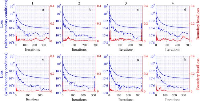
Figure 4. The loss curve: a–d are the loss curves without boundary conditions and e–h are the loss curves with boundary conditions. The blue solid line and the blue dashed line are MSE and MSEB (the left y-axis), respectively, and the red line is the ratio of MSEB to MSE (the right y-axis). |
Table 2 gives the relative errors for the four sets of numerical experiments with and without boundary condition losses corresponding to figure 4. These two cases have very similar errors. the accuracy of the solution is not affected by boundary conditions. In general, since the influence of boundary conditions on both the training process and the relative L2 errors is limited, the PIMNs is insensitive to the boundary conditions. But this does not mean that the boundary conditions are not important for solving PDEs, it only shows that the PIMNs can solve initial value problems for PDEs.
Table 2. The KdV equation: relative L2 errors with and without boundary conditions. |
| Relative L2 errors | Relative L2 errors | |
|---|---|---|
| (without boundary conditions) | (with boundary conditions) | |
| 1 | 1.690 036 × 10−3 | 9.738 059 × 10−4 |
| 2 | 8.357 186 × 10−4 | 1.799 449 × 10−3 |
| 3 | 1.661 154 × 10−3 | 1.724 861 × 10−3 |
| 4 | 1.835 814 × 10−3 | 1.678 390 × 10−3 |
3.1.3. The effect of network structure for solving the KdV equation
In this part, based on the same training data, we investigated the effect of network structure on solving the KdV equation by setting different numbers of LSTM layers and hidden nodes. Complex networks tend to be more expressive, but also more difficult to train. The relative L2 errors for different network structures are given in table 3. Among them, the number of hidden nodes does not include the last LSTM layer (the last LSTM hidden node is 1).
Table 3. The KdV equation: relative L2 errors for different network structures. |
| Neurons /layers | 2 | 3 | 4 | 5 |
|---|---|---|---|---|
| 10 | 1.795 948 × 10−3 | 1.375 186 × 10−3 | 1.483 687 × 10−3 | 1.562 139 × 10−3 |
| 30 | 9.063 210 × 10−4 | 1.149 931 × 10−3 | 1.229 779 × 10−3 | 1.364 718 × 10−3 |
| 50 | 1.162 169 × 10−3 | 5.524 451 × 10−4 | 1.071 582 × 10−3 | 1.361 776 × 10−3 |
| 70 | 1.129 416 × 10−3 | 1.078 128 × 10−3 | 1.045 698 × 10−3 | 8.195 887 × 10−4 |
Table 3 shows experimental results of different network structures. When increasing the number of LSTM layers and hidden nodes, the error shows a tendency to decrease. Although not all data fit this trend, it can still be argued that a complex network structure is beneficial to increase accuracy.
3.1.4. The effect of mesh size on solving the KdV equation
In this part, the impact of mesh size on errors is studied when the region is fixed as [−10, 10] × [0, 1]. More temporal and spatial points represent smaller temporal and spatial steps and finer grids. In general, a finer grid produces a smaller truncation error in the difference schemes. This means numerical solutions with smaller errors. But, a fine grid also represents a large amount of training data, which is more demanding to train the model. The number of spatial points is set to 500, 1000, 1500 and 2000. The number of time points is set to 50, 100, 150 and 200. The network structure is chosen with 3 LSTM layers and the first 2 layers have 50 hidden nodes.
The errors at different mesh sizes are given in table 4. It can be observed that in the case of all time nodes, the error is minimum when the spatial node is 500. However, the change of time node does not have a regular effect on the error. To sum up, excessively increasing the grid number and decreasing grid size does not improve the accuracy of the solution for a fixed region.
Table 4. The KdV equation: relative L2 errors for different mesh size. |
| Spatial points /time points | 50 | 100 | 150 | 200 |
|---|---|---|---|---|
| 500 | 9.534 459 × 10−4 | 5.069 412 × 10−4 | 5.014 334 × 10−4 | 5.628 230 × 10−4 |
| 1000 | 7.947 627 × 10−4 | 8.739 067 × 10−4 | 1.447 893 × 10−3 | 8.306 117 × 10−3 |
| 1500 | 1.884 557 × 10−3 | 2.239 517 × 10−3 | 1.932 972 × 10−3 | 3.545 602 × 10−3 |
| 2000 | 1.442 287 × 10−2 | 9.473 998 × 10−3 | 1.581 677 × 10−2 | 1.531 911 × 10−2 |
Figure 5 shows the dynamic behavior of learned solution and the error density diagram when the time points are 150 and the spatial points are 500. The number of iterations is 622 and the training time is 91 s. The error density diagram shows that the error has remained very low and has not changed significantly over time. Therefore, PIMNs can still solve the KdV equation with high accuracy when only the initial conditions are available.
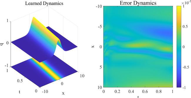
Figure 5. The traveling wave solution of the KdV equation: the dynamic behavior of learned solution and the error density diagram. |
3.1.5. Comparison of the PINNs and the PIMNs for the KdV equation
In this part, the KdV equation is solved by the PINNs and the PIMNs with and without boundary conditions, respectively. To effectively compare these two methods, three sets of comparison experiments were set up and the number of parameters of the three cases is set close to each other. The number of hidden layers of the PINNs are 5, 7, 9 and the single layer neuron is 50. The numbers of parameters are 10 401, 15 501, 20 601. The number of initial and boundary points and collocations points are 100, 10 000, respectively. The structure of the PIMNs is two LSTM layers, and the first layer is 50, 60, 70 nodes, respectively. The numbers of parameters are 10 808, 15 368, 20 728. Table 5 shows the relative errors and number of parameters for the PINNs with boundary condition losses and the PIMNs with and without boundary condition losses.
Table 5. The KdV equation: relative L2 errors for the PINNs and the PIMNs. |
| PINNs | PIMNs without boundary conditions | PIMNs with boundary conditions | ||||
|---|---|---|---|---|---|---|
| Relative L2 error | Parameters | Relative L2 error | Parameters | Relative L2 error | Parameters | |
| 1 | 1.977 253 × 10−3 | 10 401 | 7.569 623 × 10−4 | 10 808 | 5.168 963 × 10−4 | 10 808 |
| 2 | 2.700 721 × 10−3 | 15 501 | 6.007 163 × 10−4 | 15 368 | 6.046 472 × 10−4 | 15 368 |
| 3 | 1.685 079 × 10−3 | 20 601 | 5.175 313 × 10−4 | 20 728 | 5.448 766 × 10−4 | 20 728 |
In terms of the relative errors, all three cases are able to solve the KdV equation with high accuracy. Both the errors of the PIMNs with and without boundary conditions is lower than that of the PINNs when the number of parameters is close. This indicates that the structure of the PIMNs is more advantageous when reconstructing the solutions of the KdV equation. Also, consistent with the 3.1.2 subsection, the PIMNs with boundary conditions does not show a significant advantage over the PIMNs without boundary conditions. In summary, the PIMNs can simulate the solution of the KdV equation with only initial conditions, and even have higher accuracy than the PINNs.
3.2. Case 2: Nonlinear Schrödinger equation
To test the ability of the PIMNs to handle complex PDEs, the nonlinear Schrödinger equation is solved. The nonlinear Schrödinger equation is often used to describe quantum behavior in quantum mechanics and plays an important role in the physical fields such as plasma, fluid mechanics, and Bose–Einstein condensates [43, 44]. The nonlinear Schrödinger equation is given by18 ) can be referred to in the [45]. The complex value solution q is formulated as q = u + iv, and u(x, t) and v(x, t) are real-valued functions of x, t. The equation (18 ) can be converted into18 ) can be defined as21 ) is reduced to
$\begin{eqnarray}\begin{array}{rcl}{\rm{i}}{q}_{t}={q}_{{xx}}+2| q{| }^{2}q,x & \in & [{x}_{0},{x}_{1}],t\in [{t}_{0},{t}_{1}],\\ q(x,{t}_{0}) & = & {q}_{0}(x),\\ q({x}_{0},t) & = & {q}_{1}(t),\\ q({x}_{1},t) & = & {q}_{2}(t),\end{array}\end{eqnarray}$
where q are complex-valued solutions, q0(x) is an initial function, and q1(x) and q2(x) are boundary functions. The existence theory of equation ( $\begin{eqnarray}\begin{array}{rcl}{u}_{t} & = & {v}_{{xx}}+2| {u}^{2}+{v}^{2}| v,\\ {v}_{t} & = & -{u}_{{xx}}-2| {u}^{2}+{v}^{2}| u.\end{array}\end{eqnarray}$
The residuals of equation ( $\begin{eqnarray}\begin{array}{rcl}{f}_{u} & := & {u}_{t}-{v}_{{xx}}-2| {u}^{2}+{v}^{2}| v,\\ {f}_{v} & := & {v}_{t}+{u}_{{xx}}+2| {u}^{2}+{v}^{2}| u.\end{array}\end{eqnarray}$
Here, the traveling wave solution is simulated by the PIMNs and formed as $\begin{eqnarray}q(x,t)=\sqrt{c}{\rm{sech}} (\sqrt{c}(x-{vt})){{\rm{e}}}^{{\rm{i}}(-\frac{v}{2})(x-{vt})+{\rm{i}}\omega t},\end{eqnarray}$
where c = −ω − v2/4 > 0. Taking c = 0.8, v = 1.5, the traveling wave solution equation ( $\begin{eqnarray}q(x,t)=\frac{2\sqrt{5}}{5}{\rm{sech}} \left(\frac{2\sqrt{5}}{5}(x-t)\right){{\rm{e}}}^{-\tfrac{3}{4}{\rm{i}}x-\frac{49}{80}{\rm{i}}t}.\end{eqnarray}$
Taking [x0, x1], [t0, t1] as [–10, 10], [0, 1], the corresponding initial and boundary functions are obtained.3.2.1. Comparison of different difference schemes for solving the nonlinear Schrödinger equation
Similar to the KdV equation, it is first discussed that which difference schemes should be used to calculate the temporal derivatives of the solution q. The space [−10, 10] is divided into 1000 points and the time [0, 1] is divided into 100 points. Two LSTM layers are used, and the number of nodes is 30 and 2, respectively. Table 6 shows the results generated by the four sets of random numbers.
Table 6. The nonlinear Schrödinger equation: relative L2 errors for different difference schemes. |
| Difference schemes | Forward difference | Backward difference | Central difference |
|---|---|---|---|
| 1 | 2.604 364 × 10−3 | 3.259 175 × 10−3 | 1.330 293 × 10−2 |
| 2 | 3.527 666 × 10−3 | 3.842 570 × 10−3 | 2.265 705 × 10−3 |
| 3 | 2.735 975 × 10−3 | 1.453 902 × 10−2 | 2.476 216 × 10−3 |
| 4 | 1.529 878 × 10−2 | 4.381 561 × 10−3 | 1.333 741 × 10−2 |
In table 6, the bolded data are the lowest relative L2 errors produced by the same random number. It can be seen that the temporal derivatives constructed by all three difference schemes can successfully solve the nonlinear Schrödinger equation with very small relative L2 errors. And, result generated by the central difference performs better compared to the other two ways. Therefore, the central difference is used to calculate the time derivative in the subsequent subsections.
3.2.2. The effect of boundary conditions on solving the nonlinear Schrödinger equation
To investigate the effect of boundary conditions on the solution in the nonlinear Schrödinger equation, the training process and experimental results with and without boundary conditions are compared. The network structure and training data continue the previous setup. Four sets of experiments were also set up.
Figure 6 shows the loss curve of the training process. Subplots a–d show the loss curves without boundary conditions, and subplots e–h show the loss curves with boundary conditions. It is clear that the total loss convergence levels are close for the top and bottom. Although e–h have more iterations than a–d under the influence of the boundary conditions, all ratio are very low, less than 0.01. Therefore, the boundary conditions do not positively influence the training process.
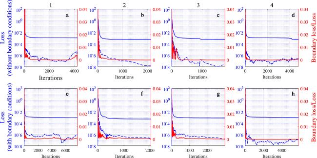
Figure 6. The loss curve: a–d are the loss curves without boundary conditions and e–h are the loss curves with boundary conditions. The blue solid line and the blue dashed line are MSE and MSEB (the left y-axis), respectively, and the red line is the ratio of MSEB to MSE (the right y-axis). |
Table 7 demonstrates the relative L2 errors with and without boundary conditions corresponding to figure 6. After adding the boundary loss to the total loss, the error is kept at the original level. The influence of the boundary conditions on the errors remains limited. Since the boundary conditions do not positively affect either the training process or the results, they are not necessary for the PIMNs.
Table 7. The nonlinear Schrödinger equation: relative L2 errors with and without boundary conditions. |
| Relative L2 errors | Relative L2 errors | |
|---|---|---|
| (without boundary conditions) | (with boundary conditions) | |
| 1 | 1.352 908 × 10−2 | 1.012 920 × 10−1 |
| 2 | 2.350 028 × 10−3 | 2.357 040 × 10−3 |
| 3 | 2.757 807 × 10−3 | 2.894 889 × 10−3 |
| 4 | 2.364 573 × 10−3 | 8.701 724 × 10−2 |
3.2.3. The effect of network structure for solving the nonlinear Schrödinger equation
In this part, we set different numbers of network layers and neurons to study that how the network structure affects the errors. The data are the same as those used before. Table 8 shows results of numerical experiments with different network structures. Note that the structures in the table 8 do not include the final LSTM layer.
Table 8. The nonlinear Schrödinger equation: relative L2 errors for different network structures. |
| Neurons/Layers | 2 | 3 | 4 | 5 |
|---|---|---|---|---|
| 10 | 2.548 948 × 10−3 | 9.138 814 × 10−4 | 1.605 489 × 10−3 | 1.609 296 × 10−3 |
| 30 | 2.434 387 × 10−3 | 2.285 506 × 10−3 | 7.020 965 × 10−4 | 2.375 666 × 10−3 |
| 50 | 2.686 936 × 10−3 | 5.575 241 × 10−4 | 5.776 256 × 10−4 | 2.827 150 × 10−3 |
| 70 | 2.246 318 × 10−3 | 6.590 603 × 10−3 | 2.362 953 × 10−3 | 2.365 898 × 10−3 |
From table 8, the error usually decreases as the number of neuron nodes and LSTM layers increases. Due to some chance factors, not all errors satisfy this law. In summary, complex structure of the PIMNs is more advantageous for solving differential equations.
3.2.4. Effect of mesh size on solving the nonlinear Schrödinger equation
In this part, we set different spatial and temporal points to study that how the mesh size affects the errors. The region remains [−10, 10] × [0, 1]. The number of spatial points is set to 500, 1000, 1500 and 2000, and the number of time points is set to 50, 100, 150 and 200. The network structure is 3 LSTM layers, and the nodes of the first two layers are 50. The relative L2 errors for different mesh sizes are given in table 9.
Table 9. The nonlinear Schrödinger equation: relative L2 errors for different mesh sizes. |
| Spatial points\Time points | 50 | 100 | 150 | 200 |
|---|---|---|---|---|
| 500 | 1.082 217 × 10−3 | 1.035 790 × 10−3 | 1.109 075 × 10−3 | 1.281 616 × 10−3 |
| 1000 | 8.084 908 × 10−3 | 8.685 522 × 10−4 | 1.072 378 × 10−3 | 8.839 646 × 10−4 |
| 1500 | 6.154 895 × 10−4 | 8.865 785 × 10−4 | 9.732 668 × 10−4 | 6.674 587 × 10−4 |
| 2000 | 6.780 904 × 10−4 | 6.010 067 × 10−4 | 7.655 602 × 10−3 | 9.272 919 × 10−3 |
As can be seen from table 9, the relative error reduces as the grid size decreases. However, the error is not minimal at a grid number of 2000 × 200. This indicates that the grid determines the relative L2 error to some extent, and moderate adjustment of the mesh size can improve the accuracy of the solution.
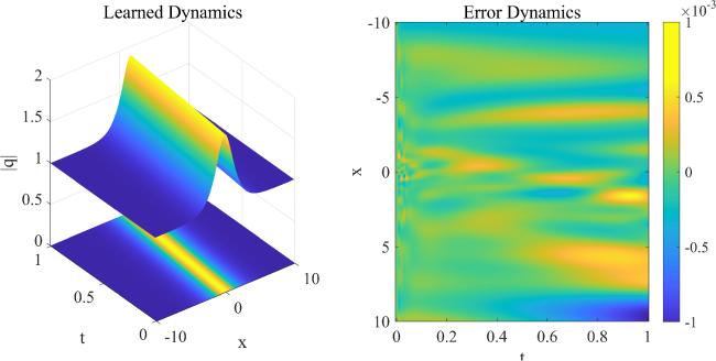
Figure 7 shows the dynamic behavior of learned solution and the error density diagram when the time points are 100 and the spatial points are 2000. The iterations are 2013 and the training time is 225 s. From the error density, although the overall level of error is low, it also demonstrates an increasing trend over time. In general, the PIMNs can solve the nonlinear Schrödinger equation with high speed and quality.
Figure 7. The traveling wave solution of the nonlinear Schrödinger equation: the dynamic behavior of learned solution and the error density diagram. |
3.2.5. Comparison of the PINNs and the PIMNs for nonlinear Schrödinger equation
In this part, the nonliner Schrödinger equation is solved using the PINNs and the PIMNs with and without boundary conditions, respectively. And the differences between the two models are discussed by comparing the relative errors. Similarly to 3.1.5, the parameters of the two models are set specifically. The PINNs has 5, 7, 9 layers with 50 nodes in each layer. The initial boundary points and the collocations points are 100 and 10 000, respectively. The PIMNs have two LSTM layers and the first layer has 50, 60, 70 nodes. Table 10 gives all the relative errors and the number of parameters.
Table 10. The nonlinear Schrödinger equation: relative L2 errors for the PINNs and the PIMNs. |
| PINNs | PIMNs without boundary conditions | PIMNs with boundary conditions | ||||
|---|---|---|---|---|---|---|
| Relative L2 error | Parameters | Relative L2 error | Parameters | Relative L2 error | Parameters | |
| 1 | 1.037 740 × 10−3 | 10 452 | 2.203 071 × 10−3 | 11 024 | 2.994 355 × 10−3 | 11 024 |
| 2 | 1.794 310 × 10−3 | 15 552 | 5.195 681 × 10−4 | 15 624 | 3.743 909 × 10−1 | 15 624 |
| 3 | 1.440 035 × 10−3 | 20 652 | 2.324 897 × 10−3 | 21 024 | 2.287 124 × 10−3 | 21 024 |
From the data of table 10, both the PINNs and PIMNs can solve the nonlinear Schrödinger equation with very low error. All errors are very close except for individual experiments. The PINNs are more advantageous at the number of parameters around 10 000 and 20 000, and the PIMNs without boundary conditions have lower errors at the number of parameters around 15 000. That is, the PIMNs without boundary conditions can obtain similar results to the PIMNs with boundary conditions. This demonstrates the powerful generalization ability of the PIMNs when there is no boundary condition.
4. Conclusion
In this paper, the PIMNs are proposed to solve PDEs by physical laws and temporal structures. Differently from the PINNs, the framework of the PIMNs is based on LSTM, which can establish the long-term dependence of the PDEs’ dynamic behavior. Moreover, the physical residuals are constructed using difference schemes, which are similar to finite difference method and bring better physical interpretation. To accelerate the network training, the difference schemes are implemented using the convolutional filter. The convolution filter is not involved in the model training and is only used to calculate the physical residuals. The performance and effectiveness of the PIMNs are demonstrated by two sets of numerical experiments. Numerical experiments show that the PIMNs have excellent prediction accuracy even when only the initial conditions are available.
However, the PIMNs use only second-order central differences and do not use higher-order difference schemes. And, solving higher-order PDEs is worth investigating. In addition, most physical information deep learning methods construct numerical solutions of PDEs. In the [46], a neural network model based on generalized bilinear differential operators is proposed to solve PDEs [46]. The method obtains a new exact network model solutions of PDEs by setting the network neurons as different functions. This proves that it is feasible to construct new exact analytical solutions of PDEs using neural networks. And how to construct new analytical solutions based on the PIMNs is a very worthwhile research problem. Compared with the fully connected structure, it is difficult to set the LSTM units in the same layer as different functions. These are the main research directions for the future.