


1. Introduction
At the scale of nuclear physics with MeV energies, atomic nuclei are always considered as finite-sized strongly correlated nucleon systems. The Hamiltonian of such many-body quantum systems is exceedingly complex and remains unknown to an extent. Fortunately, nuclei can communicate with us through some observables (nuclear data), which allow us to understand nuclear properties by comparing them with the results of some theoretical models. Of course, the direct theoretical description of nuclear properties from first principles is still rather difficult, especially for heavy nuclei. As two fundamental observables of an atomic nucleus, mass and shape play a very important role in understanding many issues in nuclear physics and astrophysics [1, 2]. The steady growth over the years in the number of nuclides whose masses have been measured has contributed immensely to our understanding of several branches of fundamental physics, cf [3]. In the processes of not only studying nuclear reaction and decay but also mapping the evolution of nuclear structure across the nuclear landscape, the effects may be most apparent in the important role that masses play [4–6]. In addition, masses are always crucial for understanding the fundamental interaction and serve as the critical inputs in the theoretical prediction of astrophysical phenomena and processes, such as the composition of neutron star crusts, x-ray burst light curves, γ-process nucleosynthesis and heavy-element synthesis [7–9]. Further experimental progress is being made in international laboratories using most performant instrumentation, and various methods of modeling applied to broader areas of the nuclear mass table are also being addressed from the aspects of theory applications.
Nuclear interaction, primarily governing the nucleon systems, has short-range properties which allow one to introduce the notion of a closed nuclear surface [10]. Outside of such a surface, the nuclear interaction rapidly dies off. Therefore, one can further define the shape with the help of the nuclear surface. It is well known that much of our understanding of the low-energy structure of nuclei hinges on such a definition [2], which plays an important role in the study of various nuclear phenomena. For instance, both the ground-state and dynamical properties of nuclei are shape dependent. Numerous experiments have indicated that the vast majority of nuclei possess either spherical or ellipsoidal (prolate or oblate) ground-state shapes. Indeed, the mechanism of spontaneous symmetry breaking allows one to represent nuclei as non-spherical shapes; although, according to the rotational symmetry of the nuclear interactions, the form of the nuclear Hamiltonians is scalar. In some special regions, other shapes, e.g. triaxial or pear-like ones, may be exhibited due to the breaking of intrinsically axial or reflection symmetries. Experimental evidence for such shapes comes from the characteristic properties of nuclear spectra, nuclear moments and electromagnetic matrix elements [11]. For instance, considerable effort has been devoted to the investigation of nuclear chirality and wobbling motion as direct evidence for triaxiality [12]. The existence of reflection asymmetry, due to the occurrence of a pear-like shape, has been established since the first identification of alternate-parity bands with enhanced E1 transitions, parity doublets and collective E3 transitions [11, 13, 14].
Theoretically, the main methods related to the calculations of nuclear masses and shapes can be roughly divided into macroscopic–microscopic (MM) models and microscopic theory, e.g. cf [15–17]. The representatives of the microscopic theories are based on the self-consistent mean-field theory, such as the energy density functional method. We adopt the MM model to perform the present investigation. In practical calculations, a critical issue will be how to select an appropriate shape parameterization, which should be both accurate and simple so as to reduce the computation to a reasonable size. Actually, the complexity of a realistic parameterization will involve a trade-off between model accuracy and computational feasibility [18]. There is no doubt that the accessibility of the corresponding parameterization will be inhibited to a large extent once the computational cost, brought by considering excessive degrees of freedom, is strongly increased. So far, several popular parameterizations are available, such as spherical harmonics [15, 19], the Cassinian ovals [20], the funny-Hills parameterization [21], the matched quadratic surfaces [22] and the generalized Lawrence shapes [12, 23, 24]. In this work, see equation (10 ) in section 2 , we define the nuclear surface with the help of the spherical-harmonic functions and introduce some ‘deformation parameters’ to express nuclear shapes [25]. These deformation parameters play an important role in reliably describing many nuclear properties, such as nuclear mass, charge radii and moments of inertia. Some deformation parameters of a deformed nucleus can be determined by scattering measurements, cf [26, 27] and references therein.
For many years, the availability of abundant experimentally measured deformation data inspired searches for some interesting systematics on nuclear shapes. More than 50 years ago, the hexadecapole deformation β4 was accurately measured by α-scattering at energies well above the Coulomb barrier for rare-earth nuclei, showing that the β4 deformations systematically evolute from positive in the light rare-earth nuclei to negative in the heavy nuclei [28]. In the lanthanide and actinide regions, the existence and importance of the hexadecapole deformation was also revealed [29, 30]. Furthermore, it is found that the β4 deformation changes from large positive values around +0.1 to large negative values around −0.1 with increasing mass number A from 152 to 180 in the lanthanide region [30]. Nowadays, the β4 measurements are still attracting considerable interest in nuclear-physics research. For instance, more recently, the importance of hexadecapole deformation in 238U was confirmed at the relativistic heavy ion collider [2] and, in the light-mass nucleus 24Mg, the hexadecapole β4 deformation was determined using quasi-elastic scattering measurements [26]. In 2022, we performed a systematic investigation on the shapes of even–even nuclei across the nuclear chart, focusing on the evolution of the β2, γ and β4 deformations under rotation [31]. Several typical β4 deformation regions were presented, agreeing with the calculations by Möller et al [15] at the ground states. Following such an investigation, we further studied the effects of hexadecapole deformations on the shapes of atomic nuclei around 230U [27]—one of the prominent β4 regions. In another recent project [32], we refitted a set of macroscopic model parameters which can improve the description of nuclear binding energies. Keeping the above facts in mind, we revisit the island of hexadecapole-deformation nuclei in the A ≈ 150 mass region of the nuclear landscape and perform an extended investigation using MM calculations, primarily paying attention to the effects of hexadecapole-deformation components on nuclear shapes and masses (nuclear binding energies). Note that, due to their simplicity and high predictive power, the MM models are still widely used; although, the self-consistent mean-field theories (e.g. Hartree–Fock and relativistic mean fields) have been well developed in past decades. Moreover, the MM models never stop developing, including the microscopic and macroscopic parts, e.g. cf [25, 32–35]. Part of the aims in this work are listed below: (1) to reproduce nuclear quadrupole deformations with two sets of Woods–Saxon (WS) parameters, and provide a comparison with experimental data and other theoretical results; (2) to improve the description of nuclear masses, by comparing with the results with and without consideration of the hexadecapole deformation; (3) to test the WS parameter sets and the present MM method to some extent.
The paper is organised as follows: in section 2 , we outline the theoretical method adopted in the present project. The results of our calculation for 148−152Ce, 150−154Nd and 152−156Sm nuclei are discussed in section 3 . Special attention is focused on nuclear shapes and masses. The effects of the hexadecapole deformation on single-particle structures and binding energy are presented and analyzed. Finally, a summary is given in section 4 .
2. Theoretical method
In this section, we will summarize the leading lines and basic definitions related to the adopted theoretical method as follows. The present calculations are performed with the help of the MM method of Strutinsky [21, 36, 37], employing phenomenological realization of the nuclear mean-field Hamiltonian with the deformed WS potential.
Within the framework of the MM model, the nuclear potential energies are usually calculated, e.g. cf [37, 38] and references therein, as4 ) respectively represent the volume energy, surface energy, symmetry energy, surface symmetry energy, Coulomb energy and correction to the Coulomb energy from surface diffuseness of the charge distribution. We adopted the new coefficients: av = −15.725, as = 18.403, asym = 118.228, aasyms = −165.496 , C = 0.719 and C4 = −0.919, in units of MeV, cf [32]. It may be worth mentioning that in the literature, the available macroscopic models generally include the standard liquid-drop model [42], finite-range droplet model [15], Lublin–Strasbourg drop model [45] and so on.
$\begin{eqnarray}{E}_{\mathrm{total}}(Z,N,\beta )={E}_{\mathrm{macro}}(Z,N,\beta )+{E}_{\mathrm{micro}}(Z,N,\beta ).\end{eqnarray}$
In general, the first term on the right-hand side represents the macroscopic liquid-drop model contribution, whereas the second one is microscopic shell corrections and pairing contributions, including the components of protons and neutrons. It should be noted that slightly different definitions for the macroscopic and microscopic energies exist, cf [15, 38–40]. In this project, we follow the definition of microscopic correction in [15, 41], $\begin{eqnarray}\begin{array}{l}{E}_{\mathrm{micro}}(Z,N,\beta )={E}_{\mathrm{def}}(Z,N,\beta )\\ \quad +{E}_{\mathrm{shell}}(Z,N,\beta )\\ \quad +{E}_{\mathrm{pair}}(Z,N,\beta ),\end{array}\end{eqnarray}$
where Edef(Z, N, β) denotes the correction, [Emacro(Z, N, β ≠ 0) − Emacro(Z, N, β = 0)], due to the deformed shape. The deformation correction energy is written as [39, 42, 43] $\begin{eqnarray}\begin{array}{l}{E}_{\mathrm{def}}(Z,N,\beta )=\{[{B}_{{\rm{S}}}(\beta )-1]\\ \quad +2\chi [{B}_{{\rm{C}}}(\beta )-1]\}{E}_{{\rm{S}}}^{(0)},\end{array}\end{eqnarray}$
where the spherical surface energy ${E}_{{\rm{S}}}^{(0)}$ and the fissility parameter χ are Z and N dependent, cf [42, 43]. The relative surface and Coulomb energies BS and BC are only functions of nuclear shape. The spherical macroscopic energy is chosen to be [33, 44] $\begin{eqnarray}\begin{array}{l}{E}_{\mathrm{macro}}(Z,N,\beta =0)={a}_{v}A+{a}_{{\rm{s}}}{A}^{2/3}\\ \quad +{a}_{\mathrm{sym}}T(T+1)/A\\ \quad +{a}_{\mathrm{syms}}T(T+1)/{A}^{4/3}+C\displaystyle \frac{{Z}^{2}}{{A}^{1/3}}\\ \quad +{C}_{4}\displaystyle \frac{{Z}^{2}}{A}.\end{array}\end{eqnarray}$
These terms of the right-hand side of equation (As seen on the right-hand side of equation (2), the last two terms Eshell(Z, N, β) and Epair(Z, N, β) can be determined solely from the single-particle levels at the corresponding nuclear shape using a shell-correction method and a pairing model. So far, several methods have been developed for calculating microscopic shell correction, such as the Strutinsky method [43], the semiclassical Wigner–Kirkwood expansion method [46, 47] and the Green’s function method [48]. In this work, we adopt the widely used Strutinsky method, in which the shell correction Eshell is defined as $\sum {e}_{k}-{\tilde{E}}_{\mathrm{Strut}}$. This can be considered as a standard method (for more details, see, e.g. [43]), though its known problems appear for mean-field potentials of finite depth as well as for nuclei close to the proton or neutron drip lines.
Since the mean field cannot adequately cover the short-range components of the nucleon–nucleon interactions, the pairing force usually becomes the most dominating residual interaction in the mean-field theory. Indeed, in the MM models, besides the shell correction, another important quantum correction is the pairing-energy contribution. Let us be reminded, as shown in [49], that various variants of the pairing-energy contribution exist in the microscopic energy calculations. For instance, several kinds of the phenomenological pairing-energy expressions are widely adopted in the applications of the MM approach [49], such as pairing correlation and pairing-correction energies, employing or not employing the particle number projection technique. In the present work, the contribution ${E}_{\mathrm{pair}}(Z,N,\hat{\beta })$ in equation (2 ) is the pairing correlation energy employing the approximately particle number projection technique, namely, the Lipkin–Nogami (LN) method [50, 51]. Such a pairing treatment can help to avoid not only the spurious pairing phase transition but also particle number fluctuation encountered in the simpler Bardeen–Cooper–Schrieffer (BCS) calculation. The LN pairing energy for the system of even–even nuclei in the “paired solution” (pairing gap Δ ≠ 0) is given by [15, 50]
$\begin{eqnarray}\begin{array}{rcl}{E}_{\mathrm{LN}} & = & \displaystyle \sum _{{\rm{k}}}2{{v}_{k}}^{2}{e}_{k}-\displaystyle \frac{{{\rm{\Delta }}}^{2}}{G}-G\displaystyle \sum _{k}{{v}_{k}}^{4}\\ & & -4{\lambda }_{2}\displaystyle \sum _{k}{{u}_{k}}^{2}{{v}_{k}}^{2},\end{array}\end{eqnarray}$
where ${{v}_{k}}^{2}$, ek, Δ and λ2 represent the occupation probabilities, single-particle energies, pairing gap and number-fluctuation constant, respectively. Correspondingly, the partner expression in the ‘no-pairing solution’ (Δ = 0) reads $\begin{eqnarray}{E}_{\mathrm{LN}}({\rm{\Delta }}=0)=\displaystyle \sum _{k}2{e}_{k}-G\displaystyle \frac{N}{2}.\end{eqnarray}$
The pairing correlation is defined as the difference between the paired solution ${E}_{\mathrm{LN}}$ and the no-pairing solution ${E}_{\mathrm{LN}}$(Δ = 0), that is, $\begin{eqnarray}\begin{array}{rcl}{E}_{\mathrm{pair}} & = & \displaystyle \sum _{k}2{{v}_{k}}^{2}{e}_{k}-\displaystyle \frac{{{\rm{\Delta }}}^{2}}{G}-G\displaystyle \sum _{k}{{v}_{k}}^{4}\\ & & -4{\lambda }_{2}\displaystyle \sum _{k}{{u}_{k}}^{2}{{v}_{k}}^{2}+G\displaystyle \frac{N}{2}-\displaystyle \sum _{k}2{e}_{k}.\end{array}\end{eqnarray}$
To clarify some confusing points, it is worth noting that in the literature, e.g. cf [52, 53], the quantum shell correction and pairing contribution are sometime merged as the ‘shell correction’ δEshell (cf equation (1) in [52], $\equiv {E}_{\mathrm{LN}}-{\tilde{E}}_{\mathrm{Strut}}$), where the definition of ${E}_{\mathrm{LN}}$ is somewhat different, including the term $G\tfrac{N}{2};$ however, the present summation Eshell + Epair agrees with the so-called ‘shell correction’ δEshell. Actually, some basic concepts, such as shell correction, pairing correlation and pairing correction, are worth paying attention to in the practical work.The single-particle levels are obtained by solving the Schrödinger equation with a self-consistent or phenomenological mean field. As is known, the applications of the three-dimensional harmonic oscillator potential, e.g. in Cartesian, cylindrical or spherical coordinates, are myriad, ranging from the usual problems in classical mechanics to more sophisticated treatments in quantum mechanics, field theory and group theory [54]. One can usually use the oscillator to obtain closed-form expressions that illustrate the general properties of a particular physical system. In nuclear physics, the harmonic oscillator has been quite successful, e.g. the important application in representing the nuclear shapes in light nuclei. However, relative to the harmonic oscillator (HO) potential, the WS mean field in a nucleus is more realistic due to its flat-bottomed and short-range properties. In this project, we numerically solve the Schrödinger equation with a phenomenological WS Hamiltonian [39, 55], which is written as,6 ) due to the different radius parameter rso. Also, the spin–orbit diffusivity parameter aso is usually updated. With the realistic WS potential modeling (e.g. considering the saturation and short-range properties of nuclear force) and model parameters (taken from [47, 56]), the WS Hamiltonian matrix can be calculated by, e.g. the numerical integral with the aid of a set of orthogonal complete bases (note that, in this case, the analytic solution to the Schrödinger equation does not exist). Then, the corresponding energy levels (eigenvalues) and wave functions (eigenvectors) are obtained using the standard diagonalization methods.
$\begin{eqnarray}{\hat{H}}_{\mathrm{WS}}=\hat{T}+{\hat{V}}_{\mathrm{cent}}+{\hat{V}}_{\mathrm{so}}+{\hat{V}}_{\mathrm{Coul}},\end{eqnarray}$
where the Coulomb potential VCoul, defined as a classical electrostatic potential of a uniformly charged drop, is added for protons. The central part of the WS potential reads $\begin{eqnarray}{\hat{V}}_{\mathrm{cent}}(\vec{r},\beta ;{V}_{0},{r}_{0},{a}_{0})=\displaystyle \frac{{V}_{0}[1\pm \kappa (N-Z)/(N+Z)]}{1+\exp [{\mathrm{dist}}_{{\rm{\Sigma }}}(\vec{r},\hat{\beta };{r}_{0})/{a}_{0}]},\end{eqnarray}$
where the plus and minus signs hold for protons and neutrons, respectively, and the parameter a0 denotes the diffuseness of the nuclear surface, which is parametrized in terms of the multipole expansion of spherical harmonics, Yλμ(θ, φ). The parameters V0 and r0 represent, respectively, the central potential depth and central potential radius parameters. The term ${\mathrm{dist}}_{{\rm{\Sigma }}}(\vec{r},\beta ;{r}_{0})$ represents the distance of a point $\vec{r}$ from the nuclear surface Σ. In principle, one can obtain the surface via different shape parameterizations. Here, we adopt the standard form of the surface definition, $\begin{eqnarray}\begin{array}{l}{\rm{\Sigma }}:R(\theta ,\phi )={r}_{0}{A}^{1/3}c(\beta )\\ \quad \times \left[1+\displaystyle \sum _{\lambda }\displaystyle \sum _{\mu =-\lambda }^{+\lambda }{\alpha }_{\lambda \mu }{Y}_{\lambda \mu }(\theta ,\phi )\right],\end{array}\end{eqnarray}$
where the function c(β) ensures the conservation of the nuclear volume, and β denotes the set of all the deformation parameters {αλμ}. The mean-field spin–orbit potential, which can strongly affect the level order and depends on the gradient of the central potential with new parameters, is defined by $\begin{eqnarray}\begin{array}{l}{\hat{V}}_{\mathrm{so}}(\vec{r},\hat{p},\hat{s},\beta ;\lambda ,{r}_{\mathrm{so}},{a}_{\mathrm{so}})\\ \quad =-\lambda {\left[\displaystyle \frac{{\hslash }}{2{mc}}\right]}^{2}{\rm{\nabla }}{V}^{\mathrm{so}}\times \hat{p}\cdot \hat{s},\end{array}\end{eqnarray}$
where $\begin{eqnarray}\begin{array}{l}{V}^{\mathrm{so}}(\vec{r},\beta ;{r}_{\mathrm{so}},{a}_{\mathrm{so}})\\ \quad =\displaystyle \frac{{V}_{0}[1\pm \kappa (N-Z)/(N+Z)]}{1+\exp [{\mathrm{dist}}_{{{\rm{\Sigma }}}_{\mathrm{so}}}(\vec{r},\beta ;{r}_{\mathrm{so}})/{a}_{\mathrm{so}}]}.\end{array}\end{eqnarray}$
The parameter λ denotes the strength of the effective spin–orbit force acting on the individual nucleons. It should be stressed that the new surface Σso is different from the one in equation (In this work, we use the eigenfunctions of the axially deformed harmonic oscillator potential in the cylindrical coordinate system as the basis function, as seen below,
$\begin{eqnarray}| {n}_{\rho }{n}_{z}{\rm{\Lambda }}{\rm{\Sigma }}\rangle ={\psi }_{{n}_{\rho }}^{{\rm{\Lambda }}}(\rho ){\psi }_{{n}_{z}}(z){\psi }_{{\rm{\Lambda }}}(\varphi )\chi ({\rm{\Sigma }}).\end{eqnarray}$
Specifically, with a set of quantum numbers {nρ, nz, Λ, Σ}, the HO wave functions can be given and used for the Hamiltonian matrix calculations (for more details, one can see, e.g. [39]). As known, the principal quantum number N meets the relationship N = 2nρ + nz + ∣Λ∣ so that the wave function ∣nρnzΛΣ > is equivalent to the notation ∣NnzΛΩ > , which is frequently used as the famous Nilsson quantum numbers. During the calculation, the eigenfunctions with N ≤ 12 and 14 are chosen as the basis set for protons and neutrons, respectively. It is found that, via such a basis cutoff, the results are sufficiently stable with respect to a possible enlargement of the basis space, indicating the completeness to some extent. In addition, the time reversal (resulting in the Kramers degeneracy) and spatial symmetries (e.g. the existence of three symmetry planes mentioned above) are used to simplify the calculations of the Hamiltonian matrix. To evaluate the effects of different deformation degrees of freedom on WS wave functions, the transformation coefficients between harmonic oscillator wave functions in different coordinate representations are derived and the corresponding codes are implanted, see the details in [54, 57]. For instance, we express the WS wave functions, calculated by the cylindrical HO basis, in the spherical HO basis ∣NljΩ > by the Moshinsky transformation (e.g. <NljΩ∣NnzΛΩ > ) instead of directly calculating them in terms of the spherical basis [54]. The notation ∣NljΩ > is equivalent to ∣nljΩ > (due to the constraint relation N = 2(n − 1) + l), which can directly run off the HO wave functions in the spherical coordinate system. Nevertheless, the WS wave functions expanded by the HO basis ∣NljΩ > , e.g. see tables 1 and 2 in the next section, are convenient for evaluating the mixing of wave functions due to the multipole interaction.Table 1. The calculated single-particle levels near the Fermi surface at β2 = 0.30, γ = 0° and β4 = 0.00 for protons and neutrons in the selected nucleus ${}_{60}^{152}$Nd92, together with their wave-function components expanded in the cylindrical basis ∣NnzΛΩ⟩ and spherical basis ∣NljΩ⟩. The calculations are performed using the WS Hamiltonian with the cranking parameters [47, 56]. The proton and neutron Fermi levels correspond to the energies −9.89 MeV and −6.37 MeV, respectively. |
| ϵ(MeV) | The former six main components in terms of ∣NnzΛΩ⟩ (upper) and ∣NljΩ⟩ (lower) | |
|---|---|---|
| Proton | −11.15 | 67.3% $| 420\tfrac{1}{2}\rangle $ + 8.9% $| 440\tfrac{1}{2}\rangle $ + 7.6% $| 431\tfrac{1}{2}\rangle $ + 4.6% $| 220\tfrac{1}{2}\rangle $ + 3.0% $| 411\tfrac{1}{2}\rangle $ + 2.4% $| 400\tfrac{1}{2}\rangle $ |
| 28.9% $| 4{d}_{5/2}\tfrac{1}{2}\rangle $ + 19.7% $| 4{g}_{7/2}\tfrac{1}{2}\rangle $ + 17.1% $| 4{s}_{1/2}\tfrac{1}{2}\rangle $ + 14.6% $| 4{g}_{9/2}\tfrac{1}{2}\rangle $ + 5.8% $| 2{s}_{1/2}\tfrac{1}{2}\rangle $ + 3.5% $| 6{d}_{5/2}\tfrac{1}{2}\rangle $ | ||
| −10.58 | 33.9% $| 550\tfrac{1}{2}\rangle $ + 28.3% $| 541\tfrac{1}{2}\rangle $ + 24.6% $| 530\tfrac{1}{2}\rangle $ + 6.7% $| 521\tfrac{1}{2}\rangle $ + 1.5% $| 510\tfrac{1}{2}\rangle $ + 1.1% $| 330\tfrac{1}{2}\rangle $ | |
| 58.4% $| 5{h}_{11/2}\tfrac{1}{2}\rangle $ + 15.2% $| 5{f}_{7/2}\tfrac{1}{2}\rangle $ + 10.7% $| 3{f}_{7/2}\tfrac{1}{2}\rangle $ + 4.9% $| 7{j}_{15/2}\tfrac{1}{2}\rangle $ + 3.6% $| 7{h}_{11/2}\tfrac{1}{2}\rangle $ + 3.1% $| 7{f}_{7/2}\tfrac{1}{2}\rangle $ | ||
| −10.37 | 98.6% $| 404\tfrac{9}{2}\rangle $ + 0.6% $| 624\tfrac{9}{2}\rangle $ + 0.5% $| 804\tfrac{9}{2}\rangle $ + 0.3% $| 604\tfrac{9}{2}\rangle $ + 0.1% $| 824\tfrac{9}{2}\rangle $ + 0.0% $| 844\tfrac{9}{2}\rangle $ | |
| 97.1% $| 4{g}_{9/2}\tfrac{9}{2}\rangle $ + 1.8% $| 6{i}_{13/2}\tfrac{9}{2}\rangle $ + 0.5% $| 6{i}_{11/2}\tfrac{9}{2}\rangle $ + 0.3% $| 8{g}_{9/2}\tfrac{9}{2}\rangle $ + 0.2% $| 10{g}_{9/2}\tfrac{9}{2}\rangle $ + 0.0% $| 6{g}_{9/2}\tfrac{9}{2}\rangle $ | ||
| −9.89 | 60.6% $| 541\tfrac{3}{2}\rangle $ + 19.4% $| 532\tfrac{3}{2}\rangle $ + 14.2% $| 521\tfrac{3}{2}\rangle $ + 1.6% $| 512\tfrac{3}{2}\rangle $ + 1.4% $| 321\tfrac{3}{2}\rangle $ + 0.7% $| 981\tfrac{3}{2}\rangle $ | |
| 64.9% $| 5{h}_{11/2}\tfrac{3}{2}\rangle $ + 13.0% $| 5{f}_{7/2}\tfrac{3}{2}\rangle $ + 8.8% $| 3{f}_{7/2}\tfrac{3}{2}\rangle $ + 5.0% $| 7{j}_{15/2}\tfrac{3}{2}\rangle $ + 2.9% $| 7{h}_{11/2}\tfrac{3}{2}\rangle $ + 2.0% $| 7{f}_{7/2}\tfrac{3}{2}\rangle $ | ||
| −8.63 | 90.5% $| 413\tfrac{5}{2}\rangle $ + 7.6% $| 422\tfrac{5}{2}\rangle $ + 0.5% $| 402\tfrac{5}{2}\rangle $ + 0.4% $| 202\tfrac{5}{2}\rangle $ + 0.4% $| 633\tfrac{5}{2}\rangle $ + 0.1% $| 813\tfrac{5}{2}\rangle $ | |
| 85.6% $| 4{g}_{7/2}\tfrac{5}{2}\rangle $ + 6.0% $| 4{g}_{9/2}\tfrac{5}{2}\rangle $ + 3.7% $| 6{i}_{11/2}\tfrac{5}{2}\rangle $ + 3.0% $| 4{d}_{5/2}\tfrac{5}{2}\rangle $ + 0.6% $| 2{d}_{5/2}\tfrac{5}{2}\rangle $ + 0.6% $| 6{i}_{13/2}\tfrac{5}{2}\rangle $ | ||
| −8.61 | 78.3% $| 532\tfrac{5}{2}\rangle $ + 12.2% $| 523\tfrac{5}{2}\rangle $ + 6.3% $| 512\tfrac{5}{2}\rangle $ + 1.2% $| 312\tfrac{5}{2}\rangle $ + 0.6% $| 752\tfrac{5}{2}\rangle $ + 0.5% $| 972\tfrac{5}{2}\rangle $ | |
| 74.5% $| 5{h}_{11/2}\tfrac{5}{2}\rangle $ + 8.9% $| 5{f}_{7/2}\tfrac{5}{2}\rangle $ + 5.7% $| 3{f}_{7/2}\tfrac{5}{2}\rangle $ + 5.0% $| 7{j}_{15/2}\tfrac{5}{2}\rangle $ + 1.9% $| 5{h}_{9/2}\tfrac{5}{2}\rangle $ + 1.6% $| 7{h}_{11/2}\tfrac{5}{2}\rangle $ | ||
| −8.16 | 83.1% $| 411\tfrac{3}{2}\rangle $ + 4.4% $| 211\tfrac{3}{2}\rangle $ + 3.5% $| 431\tfrac{3}{2}\rangle $ + 3.2% $| 422\tfrac{3}{2}\rangle $ + 2.0% $| 631\tfrac{3}{2}\rangle $ + 1.7% $| 402\tfrac{3}{2}\rangle $ | |
| 63.6% $| 4{d}_{5/2}\tfrac{3}{2}\rangle $ + 12.8% $| 4{g}_{7/2}\tfrac{3}{2}\rangle $ + 10.1% $| 4{g}_{9/2}\tfrac{3}{2}\rangle $ + 3.3% $| 4{d}_{3/2}\tfrac{3}{2}\rangle $ + 3.2% $| 2{d}_{5/2}\tfrac{3}{2}\rangle $ + 2.3% $| 6{d}_{5/2}\tfrac{3}{2}\rangle $ | ||
| Neutron | −7.31 | 83.2% $| 402\tfrac{3}{2}\rangle $ + 5.6% $| 602\tfrac{3}{2}\rangle $ + 5.1% $| 202\tfrac{3}{2}\rangle $ + 3.0% $| 411\tfrac{3}{2}\rangle $ + 2.0% $| 622\tfrac{3}{2}\rangle $ + 0.5% $| 422\tfrac{3}{2}\rangle $ |
| 74.2% $| 4{d}_{3/2}\tfrac{3}{2}\rangle $ + 8.9% $| 4{g}_{7/2}\tfrac{3}{2}\rangle $ + 7.4% $| 4{d}_{5/2}\tfrac{3}{2}\rangle $ + 3.6% $| 6{d}_{3/2}\tfrac{3}{2}\rangle $ + 2.2% $| 2{d}_{3/2}\tfrac{3}{2}\rangle $ + 0.7% $| 4{g}_{9/2}\tfrac{3}{2}\rangle $ | ||
| −6.94 | 27.0% $| 640\tfrac{1}{2}\rangle $ + 26.1% $| 651\tfrac{1}{2}\rangle $ + 24.0% $| 660\tfrac{1}{2}\rangle $ + 10.7% $| 631\tfrac{1}{2}\rangle $ + 3.2% $| 620\tfrac{1}{2}\rangle $ + 2.0% $| 880\tfrac{1}{2}\rangle $ | |
| 51.1% $| 6{i}_{13/2}\tfrac{1}{2}\rangle $ + 12.7% $| 6{g}_{9/2}\tfrac{1}{2}\rangle $ + 12.5% $| 4{g}_{9/2}\tfrac{1}{2}\rangle $ + 7.8% $| 8{i}_{13/2}\tfrac{1}{2}\rangle $ + 6.0% $| 8{g}_{9/2}\tfrac{1}{2}\rangle $ + 4.3% $| 8{k}_{17/2}\tfrac{1}{2}\rangle $ | ||
| −6.45 | 46.9% $| 651\tfrac{3}{2}\rangle $ + 22.0% $| 642\tfrac{3}{2}\rangle $ + 19.2% $| 631\tfrac{3}{2}\rangle $ + 3.5% $| 622\tfrac{3}{2}\rangle $ + 2.6% $| 871\tfrac{3}{2}\rangle $ + 1.3% $| 431\tfrac{3}{2}\rangle $ | |
| 56.3% $| 6{i}_{13/2}\tfrac{3}{2}\rangle $ + 11.7% $| 6{g}_{9/2}\tfrac{3}{2}\rangle $ + 11.2% $| 4{g}_{9/2}\tfrac{3}{2}\rangle $ + 7.4% $| 8{i}_{13/2}\tfrac{3}{2}\rangle $ + 4.8% $| 8{g}_{9/2}\tfrac{3}{2}\rangle $ + 4.5% $| 8{k}_{17/2}\tfrac{3}{2}\rangle $ | ||
| −6.37 | 96.2% $| 505\tfrac{11}{2}\rangle $ + 2.9% $| 705\tfrac{11}{2}\rangle $ + 0.8% $| 725\tfrac{11}{2}\rangle $ + 0.1% $| 905\tfrac{11}{2}\rangle $ + 0.0% $| 716\tfrac{11}{2}\rangle $ + 0.0% $| 925\tfrac{11}{2}\rangle $ | |
| 96.9% $| 5{h}_{11/2}\tfrac{11}{2}\rangle $ + 1.4% $| 7{j}_{15/2}\tfrac{11}{2}\rangle $ + 0.9% $| 7{h}_{11/2}\tfrac{11}{2}\rangle $ + 0.4% $| 7{j}_{13/2}\tfrac{11}{2}\rangle $ + 0.3% $| 11{h}_{11/2}\tfrac{11}{2}\rangle $ + 0.1% $| 9{h}_{11/2}\tfrac{11}{2}\rangle $ | ||
| −6.20 | 60.0% $| 521\tfrac{3}{2}\rangle $ + 20.1% $| 532\tfrac{3}{2}\rangle $ + 4.0% $| 741\tfrac{3}{2}\rangle $ + 3.8% $| 321\tfrac{3}{2}\rangle $ + 2.6% $| 512\tfrac{3}{2}\rangle $ + 2.3% $| 721\tfrac{3}{2}\rangle $ | |
| 32.8% $| 5{f}_{7/2}\tfrac{3}{2}\rangle $ + 28.2% $| 5{h}_{9/2}\tfrac{3}{2}\rangle $ + 9.1% $| 5{h}_{11/2}\tfrac{3}{2}\rangle $ + 7.3% $| 7{f}_{7/2}\tfrac{3}{2}\rangle $ + 7.1% $| 5{p}_{3/2}\tfrac{3}{2}\rangle $ + 3.1% $| 3{p}_{3/2}\tfrac{3}{2}\rangle $ | ||
| −5.55 | 65.4% $| 642\tfrac{5}{2}\rangle $ + 16.3% $| 633\tfrac{5}{2}\rangle $ + 11.0% $| 622\tfrac{5}{2}\rangle $ + 2.6% $| 862\tfrac{5}{2}\rangle $ + 1.2% $| 422\tfrac{5}{2}\rangle $ + 1.1% $| 613\tfrac{5}{2}\rangle $ | |
| 52.5% $| 5{h}_{9/2}\tfrac{5}{2}\rangle $ + 14.9% $| 5{f}_{7/2}\tfrac{5}{2}\rangle $ + 9.5% $| 5{f}_{5/2}\tfrac{5}{2}\rangle $ + 9.4% $| 5{h}_{11/2}\tfrac{5}{2}\rangle $ + 2.9% $| 3{f}_{5/2}\tfrac{5}{2}\rangle $ + 2.6% $| 7{j}_{13/2}\tfrac{5}{2}\rangle $ | ||
| −5.54 | 67.4% $| 523\tfrac{5}{2}\rangle $ + 16.0% $| 532\tfrac{5}{2}\rangle $ + 8.2% $| 512\tfrac{5}{2}\rangle $ + 2.8% $| 312\tfrac{5}{2}\rangle $ + 1.8% $| 503\tfrac{5}{2}\rangle $ + 1.2% $| 712\tfrac{5}{2}\rangle $ | |
| 64.8% $| 6{i}_{13/2}\tfrac{5}{2}\rangle $ + 9.7% $| 6{g}_{9/2}\tfrac{5}{2}\rangle $ + 8.6% $| 4{g}_{9/2}\tfrac{5}{2}\rangle $ + 6.5% $| 8{i}_{13/2}\tfrac{5}{2}\rangle $ + 4.6% $| 8{k}_{17/2}\tfrac{5}{2}\rangle $ + 3.0% $| 8{g}_{9/2}\tfrac{5}{2}\rangle $ |
Table 2. The same as table 1, but β4 = 0.10 and the proton and neutron Fermi levels correspond to the energies −10.50 MeV and −6.89 MeV, respectively. |
| ϵ (MeV) | The former six main components in terms of ∣NnzΛΩ⟩ (upper) and ∣NljΩ⟩ (lower) | |
|---|---|---|
| Proton | −10.99 | 82.9% $| 422\tfrac{3}{2}\rangle $ + 10.6% $| 431\tfrac{3}{2}\rangle $ + 4.1% $| 402\tfrac{3}{2}\rangle $ + 0.8% $| 211\tfrac{3}{2}\rangle $ + 0.4% $| 411\tfrac{3}{2}\rangle $ + 0.3% $| 842\tfrac{3}{2}\rangle $ |
| 67.9% $| 4{g}_{7/2}\tfrac{3}{2}\rangle $ + 13.9% $| 4{g}_{9/2}\tfrac{3}{2}\rangle $ + 6.3% $| 4{d}_{3/2}\tfrac{3}{2}\rangle $ + 4.7% $| 6{i}_{11/2}\tfrac{3}{2}\rangle $ + 2.5% $| 4{d}_{5/2}\tfrac{3}{2}\rangle $ + 1.7% $| 2{d}_{3/2}\tfrac{3}{2}\rangle $ | ||
| −10.87 | 98.4% $| 404\tfrac{9}{2}\rangle $ + 0.9% $| 604\tfrac{9}{2}\rangle $ + 0.4% $| 804\tfrac{9}{2}\rangle $ + 0.2% $| 824\tfrac{9}{2}\rangle $ + 0.0% $| 624\tfrac{9}{2}\rangle $ + 0.0% $| 1044\tfrac{9}{2}\rangle $ | |
| 99.0% $| 4{g}_{9/2}\tfrac{9}{2}\rangle $ + 0.4% $| 8{g}_{9/2}\tfrac{9}{2}\rangle $ + 0.3% $| 6{i}_{13/2}\tfrac{9}{2}\rangle $ + 0.2% $| 10{g}_{9/2}\tfrac{9}{2}\rangle $ + 0.1% $| 6{i}_{11/2}\tfrac{9}{2}\rangle $ + 0.0% $| 8{k}_{17/2}\tfrac{9}{2}\rangle $ | ||
| −10.66 | 73.3% $| 420\tfrac{1}{2}\rangle $ + 6.0% $| 431\tfrac{1}{2}\rangle $ + 5.3% $| 400\tfrac{1}{2}\rangle $ + 4.8% $| 440\tfrac{1}{2}\rangle $ + 2.9% $| 220\tfrac{1}{2}\rangle $ + 2.5% $| 411\tfrac{1}{2}\rangle $ | |
| 26.0% $| 4{d}_{5/2}\tfrac{1}{2}\rangle $ + 24.5% $| 4{g}_{7/2}\tfrac{1}{2}\rangle $ + 22.5% $| 4{g}_{9/2}\tfrac{1}{2}\rangle $ + 11.2% $| 4{s}_{1/2}\tfrac{1}{2}\rangle $ + 3.5% $| 6{d}_{5/2}\tfrac{1}{2}\rangle $ + 2.3% $| 2{s}_{1/2}\tfrac{1}{2}\rangle $ | ||
| −10.50 | 66.2% $| 541\tfrac{3}{2}\rangle $ + 12.7% $| 532\tfrac{3}{2}\rangle $ + 12.2% $| 521\tfrac{3}{2}\rangle $ + 3.4% $| 321\tfrac{3}{2}\rangle $ + 1.8% $| 761\tfrac{3}{2}\rangle $ + 1.3% $| 512\tfrac{3}{2}\rangle $ | |
| 55.0% $| 5{h}_{11/2}\tfrac{3}{2}\rangle $ + 12.2% $| 5{f}_{7/2}\tfrac{3}{2}\rangle $ + 7.9% $| 3{f}_{7/2}\tfrac{3}{2}\rangle $ + 6.5% $| 7{j}_{15/2}\tfrac{3}{2}\rangle $ + 4.3% $| 3{p}_{3/2}\tfrac{3}{2}\rangle $ + 3.9% $| 7{h}_{11/2}\tfrac{3}{2}\rangle $ | ||
| −8.30 | 80.9% $| 532\tfrac{5}{2}\rangle $ + 8.8% $| 523\tfrac{5}{2}\rangle $ + 7.6% $| 512\tfrac{5}{2}\rangle $ + 0.7% $| 752\tfrac{5}{2}\rangle $ + 0.6% $| 312\tfrac{5}{2}\rangle $ + 0.5% $| 952\tfrac{5}{2}\rangle $ | |
| 73.9% $| 5{h}_{11/2}\tfrac{5}{2}\rangle $ + 7.3% $| 5{f}_{7/2}\tfrac{5}{2}\rangle $ + 5.8% $| 7{j}_{15/2}\tfrac{5}{2}\rangle $ + 4.0% $| 3{f}_{7/2}\tfrac{5}{2}\rangle $ + 3.1% $| 5{h}_{9/2}\tfrac{5}{2}\rangle $ + 1.5% $| 7{h}_{11/2}\tfrac{5}{2}\rangle $ | ||
| −7.39 | 90.6% $| 413\tfrac{5}{2}\rangle $ + 7.3% $| 422\tfrac{5}{2}\rangle $ + 1.0% $| 402\tfrac{5}{2}\rangle $ + 0.2% $| 202\tfrac{5}{2}\rangle $ + 0.2% $| 833\tfrac{5}{2}\rangle $ + 0.2% $| 602\tfrac{5}{2}\rangle $ | |
| 84.8% $| 4{g}_{7/2}\tfrac{5}{2}\rangle $ + 7.5% $| 4{g}_{9/2}\tfrac{5}{2}\rangle $ + 4.0% $| 4{d}_{5/2}\tfrac{5}{2}\rangle $ + 2.5% $| 6{i}_{11/2}\tfrac{5}{2}\rangle $ + 0.4% $| 2{d}_{5/2}\tfrac{5}{2}\rangle $ + 0.2% $| 8{k}_{15/2}\tfrac{5}{2}\rangle $ | ||
| −7.23 | 80.9% $| 411\tfrac{3}{2}\rangle $ + 3.8% $| 422\tfrac{3}{2}\rangle $ + 3.4% $| 211\tfrac{3}{2}\rangle $ + 3.3% $| 402\tfrac{3}{2}\rangle $ + 3.3% $| 431\tfrac{3}{2}\rangle $ + 2.7% $| 651\tfrac{3}{2}\rangle $ | |
| 64.0% $| 4{d}_{5/2}\tfrac{3}{2}\rangle $ + 12.9% $| 4{g}_{7/2}\tfrac{3}{2}\rangle $ + 12.6% $| 4{g}_{9/2}\tfrac{3}{2}\rangle $ + 2.2% $| 2{d}_{5/2}\tfrac{3}{2}\rangle $ + 2.1% $| 6{g}_{9/2}\tfrac{3}{2}\rangle $ + 1.9% $| 6{d}_{5/2}\tfrac{3}{2}\rangle $ | ||
| Neutron | −7.72 | 73.0% $| 402\tfrac{3}{2}\rangle $ + 7.1% $| 602\tfrac{3}{2}\rangle $ + 5.7% $| 411\tfrac{3}{2}\rangle $ + 5.6% $| 202\tfrac{3}{2}\rangle $ + 2.3% $| 642\tfrac{3}{2}\rangle $ + 1.9% $| 651\tfrac{3}{2}\rangle $ |
| 78.2% $| 4{d}_{3/2}\tfrac{3}{2}\rangle $ + 6.4% $| 4{g}_{7/2}\tfrac{3}{2}\rangle $ + 3.6% $| 6{d}_{3/2}\tfrac{3}{2}\rangle $ + 3.0% $| 4{d}_{5/2}\tfrac{3}{2}\rangle $ + 2.9% $| 2{d}_{3/2}\tfrac{3}{2}\rangle $ + 2.5% $| 6{i}_{13/2}\tfrac{3}{2}\rangle $ | ||
| −7.64 | 62.5% $| 532\tfrac{3}{2}\rangle $ + 18.9% $| 541\tfrac{3}{2}\rangle $ + 7.4% $| 512\tfrac{3}{2}\rangle $ + 3.7% $| 521\tfrac{3}{2}\rangle $ + 3.0% $| 321\tfrac{3}{2}\rangle $ + 1.2% $| 752\tfrac{3}{2}\rangle $ | |
| 39.0% $| 5{h}_{9/2}\tfrac{3}{2}\rangle $ + 17.5% $| 5{h}_{11/2}\tfrac{3}{2}\rangle $ + 15.1% $| 5{f}_{5/2}\tfrac{3}{2}\rangle $ + 5.3% $| 3{f}_{5/2}\tfrac{3}{2}\rangle $ + 5.2% $| 5{f}_{7/2}\tfrac{3}{2}\rangle $ + 3.9% $| 7{h}_{9/2}\tfrac{3}{2}\rangle $ | ||
| −7.22 | 51.3% $| 651\tfrac{3}{2}\rangle $ + 15.0% $| 631\tfrac{3}{2}\rangle $ + 14.0% $| 642\tfrac{3}{2}\rangle $ + 5.0% $| 871\tfrac{3}{2}\rangle $ + 4.8% $| 402\tfrac{3}{2}\rangle $ + 3.5% $| 431\tfrac{3}{2}\rangle $ | |
| 43.0% $| 6{i}_{13/2}\tfrac{3}{2}\rangle $ + 10.5% $| 6{g}_{9/2}\tfrac{3}{2}\rangle $ + 9.3% $| 4{g}_{9/2}\tfrac{3}{2}\rangle $ + 8.0% $| 8{i}_{13/2}\tfrac{3}{2}\rangle $ + 7.6% $| 4{d}_{5/2}\tfrac{3}{2}\rangle $ + 5.7% $| 8{g}_{9/2}\tfrac{3}{2}\rangle $ | ||
| −6.89 | 95.4% $| 505\tfrac{11}{2}\rangle $ + 4.5% $| 705\tfrac{11}{2}\rangle $ + 0.1% $| 925\tfrac{11}{2}\rangle $ + 0.0% $| 905\tfrac{11}{2}\rangle $ + 0.0% $| 725\tfrac{11}{2}\rangle $ + 0.0% $| 716\tfrac{11}{2}\rangle $ | |
| 98.3% $| 5{h}_{11/2}\tfrac{11}{2}\rangle $ + 1.1% $| 7{h}_{11/2}\tfrac{11}{2}\rangle $ + 0.2% $| 11{h}_{11/2}\tfrac{11}{2}\rangle $ + 0.2% $| 7{j}_{15/2}\tfrac{11}{2}\rangle $ + 0.1% $| 9{h}_{11/2}\tfrac{11}{2}\rangle $ + 0.0% $| 7{j}_{13/2}\tfrac{11}{2}\rangle $ | ||
| −5.62 | 69.0% $| 642\tfrac{5}{2}\rangle $ + 12.1% $| 633\tfrac{5}{2}\rangle $ + 11.0% $| 622\tfrac{5}{2}\rangle $ + 3.6% $| 862\tfrac{5}{2}\rangle $ + 1.9% $| 422\tfrac{5}{2}\rangle $ + 1.1% $| 613\tfrac{5}{2}\rangle $ | |
| 60.7% $| 6{i}_{13/2}\tfrac{5}{2}\rangle $ + 9.0% $| 6{g}_{9/2}\tfrac{5}{2}\rangle $ + 7.1% $| 4{g}_{9/2}\tfrac{5}{2}\rangle $ + 6.7% $| 8{i}_{13/2}\tfrac{5}{2}\rangle $ + 5.7% $| 8{k}_{17/2}\tfrac{5}{2}\rangle $ + 3.0% $| 8{g}_{9/2}\tfrac{5}{2}\rangle $ | ||
| −5.50 | 63.4% $| 521\tfrac{3}{2}\rangle $ + 16.0% $| 532\tfrac{3}{2}\rangle $ + 3.7% $| 501\tfrac{3}{2}\rangle $ + 3.0% $| 321\tfrac{3}{2}\rangle $ + 2.6% $| 512\tfrac{3}{2}\rangle $ + 2.5% $| 721\tfrac{3}{2}\rangle $ | |
| 36.2% $| 5{f}_{7/2}\tfrac{3}{2}\rangle $ + 26.6% $| 5{h}_{9/2}\tfrac{3}{2}\rangle $ + 13.2% $| 5{h}_{11/2}\tfrac{3}{2}\rangle $ + 7.9% $| 7{f}_{7/2}\tfrac{3}{2}\rangle $ + 4.9% $| 5{p}_{3/2}\tfrac{3}{2}\rangle $ + 2.4% $| 3{f}_{7/2}\tfrac{3}{2}\rangle $ | ||
| −4.52 | 61.9% $| 523\tfrac{5}{2}\rangle $ + 13.9% $| 532\tfrac{5}{2}\rangle $ + 12.5% $| 512\tfrac{5}{2}\rangle $ + 5.2% $| 503\tfrac{5}{2}\rangle $ + 2.5% $| 312\tfrac{5}{2}\rangle $ + 2.0% $| 712\tfrac{5}{2}\rangle $ | |
| 47.2% $| 5{h}_{9/2}\tfrac{5}{2}\rangle $ + 22.2% $| 5{f}_{7/2}\tfrac{5}{2}\rangle $ + 14.8% $| 5{h}_{11/2}\tfrac{5}{2}\rangle $ + 4.9% $| 5{f}_{5/2}\tfrac{5}{2}\rangle $ + 2.5% $| 7{j}_{13/2}\tfrac{5}{2}\rangle $ + 2.4% $| 7{f}_{7/2}\tfrac{5}{2}\rangle $ |
In principle, after performing the above calculations of the standard several steps (as summarized in, e.g. [32, 58, 59]), the total potential energy can be obtained at each sampling grid in the selected deformation space. Then, with the aid of the interpolation (e.g. a spline function) and projection techniques, the smoothly two-dimensional potential-energy surfaces/maps in any two deformation coordinates can be obtained using the available grid data. Note that one can conveniently search the global minimum and evaluate the properties of the nuclear potential landscape based on the smooth potential-energy surfaces. Further, the equilibrium deformations, shape co-existance, fission path and other physical quantities/processes can be investigated.
3. Results and discussion
During the practical calculations of potential-energy surfaces, which are very helpful for understanding nuclear structure properties from different deformation degrees of freedom, one has to select a limited deformation space, usually 3–5 dimensions for the general computational conditions. The nuclei generally prefer to possess x − y, y − z and x − z plane-symmetries, which practically determine that nonvanishing multipole moments have λ and μ both even, e.g. cf equation (10 ). Accordingly, we impose a few symmetry restrictions on the nuclear shape in the present work. Based on the adopted shape parametrization, the quadrupole and hexadecapole-deformation degrees of freedom, including nonaxial deformations (i.e. β ≡ (α20, α2±2, α40, α4±2, α4±4)), are taken into account. In addition, according to the well-known Bohr’s (β2, γ) parametrization [60], the collective coordinates {α20, α2±2} meet the following relation
$\begin{eqnarray}\left\{\begin{array}{l}{\alpha }_{20}={\beta }_{2}\cos \gamma \\ {\alpha }_{22}={\alpha }_{2-2}=-\displaystyle \frac{1}{\sqrt{2}}{\beta }_{2}\sin \gamma .\end{array}\right.\end{eqnarray}$
By considering the Lund convention [61], we have $\begin{eqnarray}\left\{\begin{array}{l}X={\beta }_{2}\sin (\gamma +30^\circ )\\ Y={\beta }_{2}\cos (\gamma +30^\circ ).\end{array}\right.\end{eqnarray}$
As typical examples, in figure 1, the potential-energy surfaces calculated on the (X, Y), (β2, γ) and (α20, α22) planes are illustrated for the selected central nucleus ${}_{60}^{152}$Nd92. These three kinds of energy maps are all widely used in the literature. Figure 1(a) adopts the transformed quadrupole coordinates (X, Y), which are more convenient for illustrating the cranking energy surface. Under rotation, the parameter γ covers [−120°, 60°] and is divided into three sectors ([−120°, −60°], [−60°, 0°], [0°, 60°]), which respectively denotes rotation about the long intermediate and short axes, cf, e.g. [62, 63]. Figure 1(b) directly takes the β2 and γ deformation variables as the horizontal and vertical coordinates in a Cartesion coordinate system, instead of the (β2, γ) plane in the polar coordinate system. For the static energy surfaces, the γ domain [−60°, 60°] is adopted to guiding eyes, though, in principle, half is enough. These two maps are equivalent but the later can display the triaxial effect better, especially at the weak β2 deformation. Note that the proportion between β2 and γ is arbitrary due to their different ‘dimensions’ (β2 and γ respectively specify the magnitude of the quadrupole deformation and the asymmetry of the shape). In figure 1(c), the direct quadrupole deformation parameters (α20, α22) are adopted as the horizontal and vertical coordinates of the energy surface, which are widely used in the literature, cf e.g. [25, 49]. It is further worth noting that, in figure 1, the three minima possess the same energies (for display purposes, the energies at each map are respectively normalized to their minima) and equilibrium shapes, though the adopted ‘coordinates’ are somewhat different (but equivalent). Of course, one may notice that the calculated result (e.g. β2 = 0.22) in the two-dimensional deformation subspace is not in agreement with the data (experimental β2 = 0.34 [64]). The test of an extended deformation subspace, generally, including other low-order (e.g. hexadecapole) deformations, should be necessary.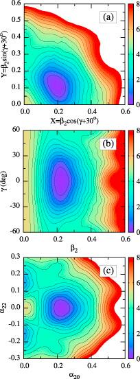
Figure 1. Illustrations of calculated two-dimensional energy surfaces, with contour-line separations of 0.5 MeV, based on quadrupole (or generalized quadrupole)-deformation coordinates (X, Y) (a), (β2, γ) (b) and (α20, α22) (c) planes in Cartesian coordinate systems for the selected nucleus ${}_{60}^{152}$Nd192. Note that the energy has already been subtracted from the minimum value (the same value in each subplot). Let us note that, in (a), (b) and (c), the equilibrium deformations (X = 0.20; Y = 0.12), (β2 = 0.22; γ = 0°) and (α20 = 0.22; α22 = 0.00) are equivalent, as expected. See the text for more details. |
Since the nucleus ${}_{60}^{152}$Nd92 has no prominent triaxiality, as seen in figure 1, to check whether the different hexadecapole-deformation degrees of freedom have an important influence on nuclear potential energies, figure 2 presents the two-dimensional energy surfaces, taking the quadrupole α20 and hexadecapole α4μ=0,2,4 deformation parameters as the coordinate axes. For simplicity, other deformation parameters are ignored during the energy calculations. It can be seen that the non-zero axially hexadecapole deformation α40(≈ 0.1) appears and the nonaxial α42 and α44 deformations prefer to zero. Furthermore, the energy minimum in figure 2(a) is about 2.7 MeV lower than those in figures 2(b) and (c), indicating that the α40 deformation may cause a large reduction in energy. The β2 deformation increases from 0.22 to 0.26, which is more close to the data. Indeed, figure 2 illustrates the hexadecapole deformations become non-negligible, especially the axial one, α40.
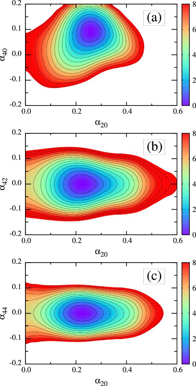
Figure 2. Similar to the preceding illustration in figure 1, but based on quadrupole and hexadecapole-deformation degrees of freedom (α20, α40) (a), (α20, α42) (b) and (α20, α44) (c) for ${}_{60}^{152}$Nd92. |
In fact, the complexity of the nuclear shape (equivalently, the intrinsic body-frame multipole moments) is associated with nuclear interaction. It is impossible to calculate in the full space expanded by the spherical harmonics, as seen in equation (10 ), which is, in principle, infinite. The reasonable selection of the deformation subspace in different mass regions and/or different spin and excitation conditions is worth exploring besides depending on experience. Following, e.g. [47], we introduce the deformation parameter β4, which obeys the relationship
$\begin{eqnarray}\left\{\begin{array}{l}{\alpha }_{40}=\displaystyle \frac{1}{6}{\beta }_{4}(5{\cos }^{2}\gamma +1)\\ {\alpha }_{42}={\alpha }_{4-2}=-\displaystyle \frac{1}{12}\sqrt{30}{\beta }_{4}\sin 2\gamma \\ {\alpha }_{44}={\alpha }_{4-4}=\displaystyle \frac{1}{12}\sqrt{70}{\beta }_{4}{\sin }^{2}\gamma .\end{array}\right.\end{eqnarray}$
The βλ is the total deformation at order λ (here λ = 4) which can, as described in [2], be defined by ${\beta }_{\lambda }=\sqrt{{\sum }_{\mu =-\lambda }^{\mu =+\lambda }{\alpha }_{\lambda \mu }^{2}}$. Under strict assumptions, one can infer the deformation of an even–even nucleus from ground-state electric transition rates, B(Eλ), by ${\beta }_{\lambda }=\tfrac{4\pi }{(2\lambda +1){{ZR}}_{0}^{\lambda }}\sqrt{B(E\lambda )/{e}^{2}}$ (see, e.g. [2]). To synthetically consider the different hexadecapole deformation degrees of freedom, we performed the realistic total energy calculations using the deformed WS mean-field Hamiltonian in the deformation space (β2, γ, β4), which is widely used in the literature. Any two-dimensional map in such a space has been illustrated in figure 3. In each subfigure, the energy is minimized over the remaining deformation degree of freedom (for instance, on the β2-vs-γ plane, the energy is minimized over β4). Similar to figure 1, the three minima on the (β2,γ), (β4,γ) and (β2,β4) planes have the same energies and correspond to the same shape. However, by comparing figure 3(a) with figure 1(b), and figure 3(c) with figure 2(a), we find that the minimization over the third deformation can modify the energy surface.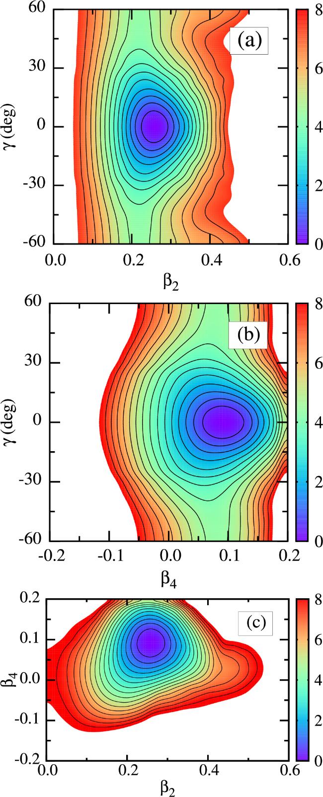
Figure 3. Projections of total energy on the (β2,γ) (a), (β4,γ) (b) and (β2,β4) (c) planes, minimized respectively at each deformation point over the remaining deformations, β4, β2 and γ. Note that the total energy is calculated in the three-dimensional deformation space (β2,γ, β4), and normalization is specified by setting the energy equal to zero at the minimum position. |
The single-particle levels determine the nuclear internal structure and microscopic shell- and pairing-correction energies. To examine the single-particle spectrum in the vicinity of the Fermi surfaces, we have calculated proton and neutron levels, which correspond to the eigenstates of the one-body WS Hamiltonian, as shown in figure 4. In the spherical case, e.g. at β2 = 0.0 in figure 4 (a) and (c), the principal quantum number n, the orbital angular momentum l and the total angular momentum j are adopted as the labels of the single-particle states. Note that, following the notations in atomic spectroscopy, the symbols s, p, d, ⋯respectively correspond to l = 0, 1, 2, ⋯. The strong spin–orbit interaction splits the l orbital into two j levels (namely, j = l ± 1/2), and each j orbital has 2j + 1 degenerate states. The high-j orbital often appears in the neighboring lower-N shell as the intruder state, e.g. cf the 1h11/2 or 1i13/2 orbital in figure 4. As expected, it can be seen that the spherical shell gaps, e.g. Z = 50 and N = 82, are reproduced at β2 = 0.0. When the spherical symmetry breaks, the orbital labeled by nlj splits into j + 1/2 components and each one is typically double degenerate due to Kramers degeneracy [27]. Let us remind ourselves that the virtual crossings of single-particle levels with the same symmetries are not removed [65], but this will not prevent the level identification. Figure 4 indicates that β4 deformation plays a critical role during the shell evolution. For example, the shell gap does not evolve at β2 ≈ 0.30 near the Fermi surface for both protons and neutrons but clearly appears at, e.g. β4 ≈ 0.10, agreeing with the calculated deformations (e.g. cf table 3).
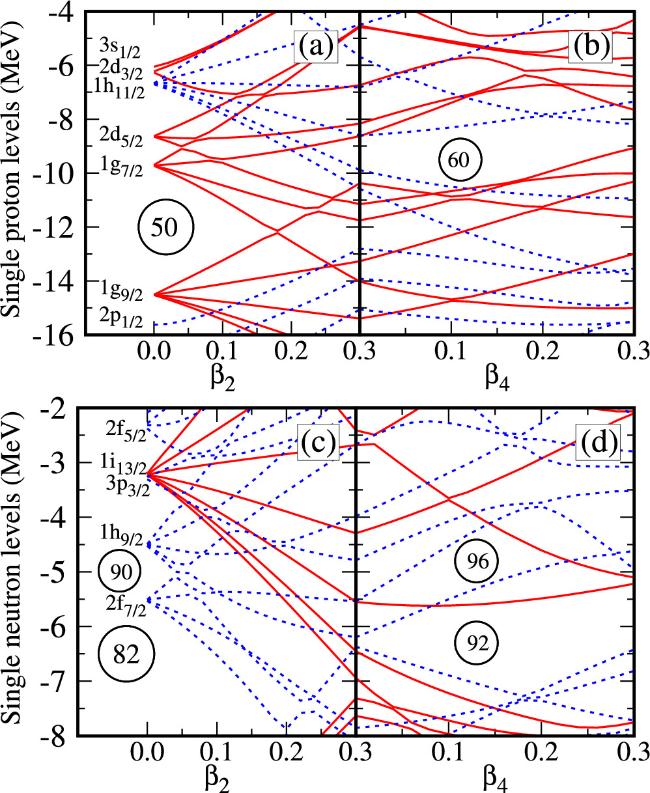
Figure 4. Calculated proton (top) and neutron (bottom) single-particle energies (in the window of interest) as functions of the quadrupole deformation β2 (left) and hexadecapole deformation β4 for ${}_{60}^{152}$Nd92, focusing on the domain near the Fermi surface. Red solid (blue dotted) lines refer to positive and negative parity. The single-particle orbitals at β2=0.0 are labelled by the spherical quantum numbers nlj; for further details, e.g. see tables 1 and 2. |
Table 3. The calculated (Cal.) equilibrium deformation parameters β2 and β4 at ground states for even–even nuclei 148−152Ce, 150−154Nd and 152−156Sm, together with the FY+FRDM (FF) [15], HFBCS [66], and ETFSI [67] calculations and partial experimental (Exp.) β2 values [64] for comparison. |
| Nuclei | β2 | β4 | |||||||||
|---|---|---|---|---|---|---|---|---|---|---|---|
| Cal.1a | Cal.2 | FF | HFBCS | ETFSI | Exp. | Cal.1 | Cal.2 | FF | HFBCS | ETFSI | |
| ${}_{58}^{148}$Ce90 | 0.212 | 0.209 | 0.216 | 0.22 | 0.24 | 0.255 | 0.076 | 0.067 | 0.109 | 0.02 | 0.06 |
| ${}_{58}^{150}$Ce92 | 0.242 | 0.235 | 0.252 | 0.25 | 0.26 | 0.317 | 0.092 | 0.082 | 0.126 | 0.02 | 0.07 |
| ${}_{58}^{152}$Ce94 | 0.255 | 0.251 | 0.261 | 0.27 | 0.28 | 0.429 | 0.086 | 0.079 | 0.111 | 0.02 | 0.06 |
| ${}_{60}^{150}$Nd90 | 0.240 | 0.235 | 0.243 | 0.25 | 0.26 | 0.283 | 0.085 | 0.076 | 0.107 | 0.02 | 0.07 |
| ${}_{60}^{152}$Nd92 | 0.262 | 0.256 | 0.262 | 0.27 | 0.29 | 0.348 | 0.095 | 0.085 | 0.128 | 0.02 | 0.07 |
| ${}_{60}^{154}$Nd94 | 0.271 | 0.268 | 0.270 | 0.29 | 0.29 | 0.258 | 0.085 | 0.080 | 0.114 | 0.02 | 0.07 |
| ${}_{62}^{152}$Sm90 | 0.242 | 0.238 | 0.243 | 0.23 | 0.26 | 0.306 | 0.071 | 0.066 | 0.090 | 0.01 | 0.05 |
| ${}_{62}^{154}$Sm92 | 0.266 | 0.262 | 0.270 | 0.27 | 0.28 | 0.340 | 0.081 | 0.074 | 0.113 | 0.01 | 0.06 |
| ${}_{62}^{156}$Sm94 | 0.276 | 0.274 | 0.279 | 0.29 | 0.30 | — | 0.077 | 0.071 | 0.098 | 0.01 | 0.05 |
aCal.1 and Cal.2 respectively indicate that the corresponding deformation parameters are calculated using the cranking and universal WS parameter sets. |
As is known, a set of conserved quantum numbers, which are associated with a complete set of commuting observables, can be used to label the corresponding single-particle levels and wave functions. As mentioned in section 2 , the WS wave functions are finally expressed by a set of HO bases. The maximum HO component is usually taken as the label of the corresponding single-particle level. In a quadrupole-deformed nucleus, the asymptotic Nilsson quantum numbers Ωπ[NnzΛ] are often adopted, where N, nz, Λ and Ω respectively stand for the total oscillator shell quantum number, the number of oscillator quanta in the z direction (the direction of the symmetry axis), the projection of orbital angular momentum along the symmetry axis and the projection of total angular momentum (cf, e.g. [27]). It needs to be stressed that once the shape becomes somewhat complicated, the so-called main component of the wave function may not be prominent any more and the label will be meaningless in principle. To understand the single-particle states and the mechanism of nuclear deformations, at two selected shapes (namely, (β2, γ, β4) = (0.3,0°, 0.0) and (0.3,0°, 0.1)), tables 1 and 2 present the calculated single-particle levels and corresponding wave functions expanded on the cylindrical and spherical HO bases, including the proton and neutron states near the Fermi surfaces. The latter is convenient for evaluating the multiple interactions which lead to the mixing of wave functions. For instance, the octupole–octupole interaction mixes the states with ΔN = 1 and Δl = Δj = 3 [11]. By combining figure 4 and these two tables, one can easily identify the asymptotic Nilsson quantum numbers of these levels at the given deformations. By comparing tables 1 and 2, one can find that the hexadecapole deformation β4 ≈ 0.1, corresponding to the hexadecapole–hexadecapole interaction, leads to the mixing of the single-particle states with Δl = Δj = 4. As expected, from these two tables, we can see that the parity and Ω are conserved due to the existence of space-reflection and axial symmetries.
Figure 5 illustrates the further evolution information on the calculated microscopic energy and its different components in functions of β2, γ and β4 for the example nucleus ${}_{60}^{152}$Nd92, primarily aiming at seeing the impact of triaxial γ and hexadecapole β4 deformations on these energies. Note that during the calculation of the corresponding energy along one deformation degree of freedom, the other two are fixed at the positions of, e.g. the equilibrium deformations, as seen in figure 5. One can see that the deformation energy smoothly increases with increasing β2 deformation and is not sensitive to triaxial deformation γ. In the β4 direction, the deformation energy seems to be more stiff. The shell correction, exhibiting a large change, determines the equilibrium position (minimum) of the microscopic energy to a large extent. As defined in section 2 , one can observe that the spherical macroscopic energy has nothing to do with the shape of the potential-energy surface. The pairing correlation energy is always negative and has a slight staggering characteristic.
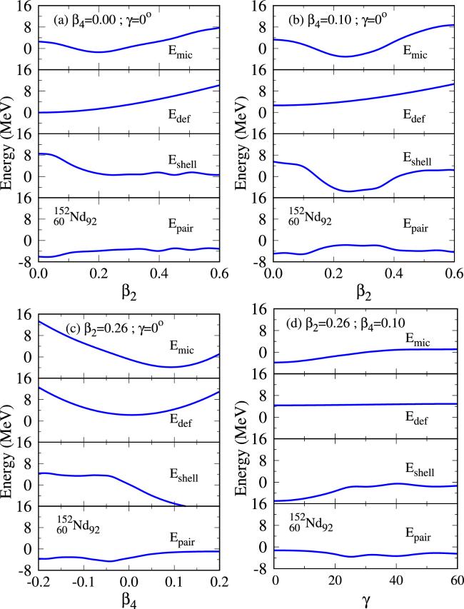
Figure 5. Calculated microscopic energies Emic, following the definition in [15, 41], in functions of different deformation degrees of freedom, together with their deformation energy Edef, quantum shell correction Eshell and pairing-energy contribution Epair, for the selected nucleus ${}_{60}^{152}$Nd92; see the text for further comments. |
To investigate the minimum properties (e.g. the depth and stiffness) near the equilibrium deformations at the selected space, figure 6 shows four types of microscopic energy curves in functions of β2 for the nuclei 148,150,152Ce, 150,152,154Nd and 152,154,156Sm. In figures 6(a) and (b), the cranking and universal WS parameter sets [39, 47, 56] are adopted, respectively. It should be noted that the energies on the black lines are minimized over both γ and β4 deformations, certainly occupying the lowest positions in each subfigure. In contrast, the highest red lines include neither γ nor β4 minimization. In addition, for the lines in other colors, the energy minimizations are performed along either the γ (blue) or β4 (green) directions. From these curves, we can adequately evaluate the effects of γ and/or β4 on nuclear potential-energy surfaces. Near the minima, one can systematically find that the black and red lines respectively overlap with the green and blue lines, indicating the neglectable (non-neglectable) effects of the triaxial γ (hexadecapole β4) deformation. Relative to the curves with β4 = 0.0, the minimum energies decrease by 1-3 MeV, and the quadrupole β2 deformations have a systematic increase due to the β4 minimization. The point with β4 ≈ 0.4 looks to be critical, where these four curves cross one another. Furthermore, after this, the triaxial γ deformation plays an important role instead of β4 (e.g. driving the energy to decrease).
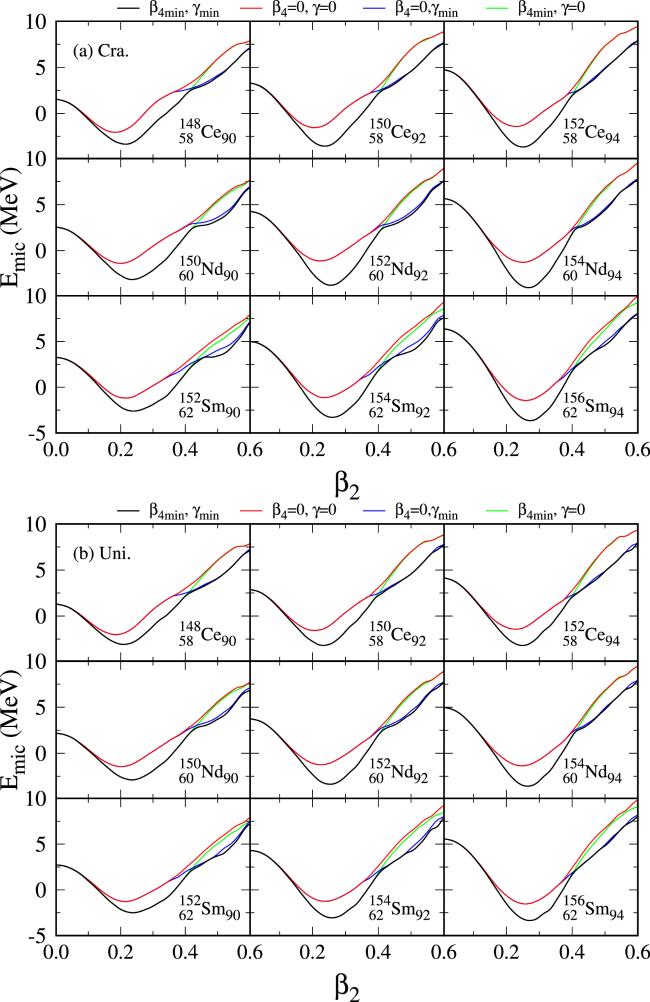
Figure 6. Four types of deformation energy curves, calculated by ‘cranking’ (top) and ‘universal’ (bottom) WS parameters [39, 47, 56], as the function of quadrupole deformation β2 for 9 nuclei 148,150,152Ce, 150,152,154Nd and 152,154,156Sm. Let us note that the lines with different colors, as denoted by the legends, represent whether or not the total energy at each β2 grid is minimized over other deformation parameter(s). For more details, see the text. |
By considering two sets of frequently used WS potential parameters, we present the calculated quadrupole deformation β2 and hexadecapole deformation β4 in table 3 for nine even–even nuclei on the selected β4 deformation island (see figure 3 in [34] for a systematic comparision with more data). As seen above, e.g. in figure 6, we see that the inclusion of β4 deformation is actually very necessary to reproduce the experimental β2 value and/or other theoretical results. For comparison, the available experimental data [64] and/or the results given by other accepted theories, such as the fold-Yukawa (FY) single-particle potential and the finite-range droplet model (FRDM) [15], the Hartree–Fock-BCS (HFBCS) [66] and the extended Thomas–Fermi plus Strutinsky integral (ETFSI) methods [67], are shown as well. It seems that these calculated results are somewhat parameter- and model-dependent but in basic agreement with one another. From this table, we can see that all the theoretical results, including both the phenomenological and the self-consistent mean-field calculations, underestimated the experimental data. Our calculated results with the cranking parameters are slightly larger than those with the universal parameters. Relatively, the ETFSI and HFBCS calculations respectively give the largest β2 and the smallest β4 values. The underestimated quadrupole deformation β2 was discussed, and the empirically modified formula, 1.10β2-$0.03{\left({\beta }_{2}\right)}^{3}$, was suggested in [68]. In addition, the β2 underestimations, especially in the soft nuclei, may to some extent originate from the dynamical effects (e.g. the vibrating coupling, cf [32, 58] for a recent discussion).
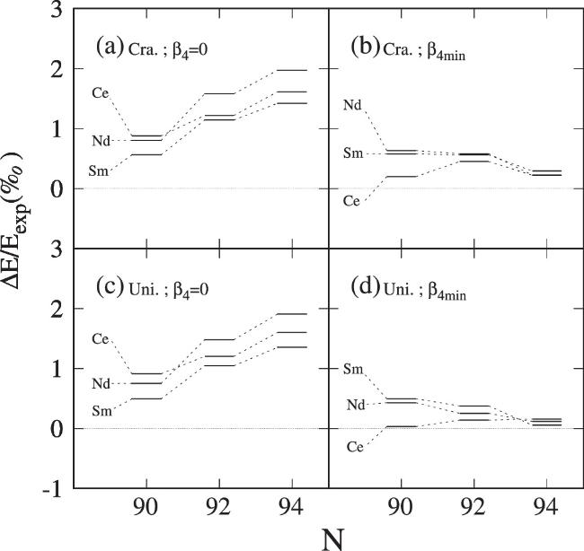
Besides the nuclear shapes, we also investigate the mass (equivalently, the binding energy, defined as negative) of the selected nuclei, as shown in table 4, in terms of the updated model parameters of the spherical macroscopic energy [32]. To quantitatively evaluate the dependence of mass on β4 deformation and WS parameter sets [39, 47, 56], we calculate the macroscopic, microscopic, total energies and the deviations between theory and experiment of four combinations based on two sets of widely used potential parameters with and without the inclusion of β4 minimization. The mass deviations obviously decrease after taking the β4 minimization into account. Relatively, the results obtained from the universal parameter set exhibit smaller mass deviations. In figure 7, the calculated permillage error of nuclear masses between theory and experiment are illustrated. One can see that the inclusion of β4 is important for reproducing the experimental data; for example, the relative errors decrease to no more than 0.1%. For these three isotopic chains, the relative mass-derivations increase (decrease) with increasing neutron number N before(after) considering the minimization over β4. The missing octupole–octupole correlation in the present calculation may affect the mass accurancy in the N = 90 (close to the octupole magic number [11]) isotones. Further study may be meaningful in an extended deformation space (e.g. including the reflection asymmetric deformation β3).
Figure 7. The calculated relative mass deviation (e.g. permillage error) between theory and experiment, with (b, d)/without (a, c) the inclusion of hexadecapole deformation β4, based on the cranking (a, b) and universal (c, d) parameter sets for 148,150,152Ce, 150,152,154Nd and 152,154,156Sm. See the text for more details. |
Table 4. The calculated macroscopic energy Emac, microscopic energy Emic, total energy Etot, experimental binding energy [3] ${E}_{\exp }$ and the deviation ΔE ($\equiv | {E}_{\mathrm{tot}}-{E}_{\exp }| $) between theory and experiment. The quantities with the superscripts a and b respectively correspond to the calculated results with cranking and universal WS parameter sets [39, 47, 56]. The italic denotes that the corresponding value is calculated without the inclusion of β4 deformation. All energies are in units of MeV. |
| Nuclear | Emac | ${E}_{\mathrm{mic}}^{a}$ | ${E}_{\mathrm{mic}}^{b}$ | ${E}_{\mathrm{tot}}^{a}$ | ${E}_{\mathrm{tot}}^{b}$ | ${E}_{\exp }$ | ΔEa | ΔEb |
|---|---|---|---|---|---|---|---|---|
| ${}_{58}^{148}$Ce90 | −1216.659 | −3.4065 | −3.1218 | −1220.066 | −1219.781 | −1219.577 | 0.489 | 0.204 |
| −2.0900 | −2.0509 | −1218.749 | −1218.710 | 0.828 | 0.867 | |||
| ${}_{58}^{150}$Ce92 | −1227.382 | −3.6231 | −3.2431 | −1231.005 | −1230.625 | −1230.168 | 0.837 | 0.457 |
| −1.5689 | −1.5888 | −1228.951 | −1228.971 | 1.217 | 1.197 | |||
| ${}_{58}^{152}$Ce94 | −1237.363 | −3.7043 | −3.2320 | −1241.067 | −1240.595 | −1240.472 | 0.595 | 0.123 |
| −1.4279 | −1.4396 | −1238.791 | −1238.803 | 1.681 | 1.669 | |||
| ${}_{60}^{150}$Nd90 | −1235.230 | −3.1964 | −2.9452 | −1238.426 | −1238.175 | −1237.437 | 0.989 | 0.738 |
| −1.4168 | −1.4805 | −1236.647 | −1236.711 | 0.790 | 0.726 | |||
| ${}_{60}^{152}$Nd92 | −1247.183 | −3.8363 | −3.4281 | −1251.019 | −1250.611 | −1250.049 | 0.970 | 0.562 |
| −1.1339 | −1.2594 | −1248.317 | −1248.442 | 1.732 | 1.607 | |||
| ${}_{60}^{154}$Nd94 | −1258.374 | −4.0602 | −3.6251 | −1262.434 | −1261.999 | −1261.867 | 0.567 | 0.132 |
| −1.2854 | −1.3667 | −1259.659 | −1259.741 | 2.208 | 2.126 | |||
| ${}_{62}^{152}$Sm90 | −1251.384 | −2.6054 | −2.5019 | −1253.989 | −1253.886 | −1253.097 | 0.892 | 0.789 |
| −1.1745 | −1.2600 | −1252.559 | −1252.644 | 0.538 | 0.453 | |||
| ${}_{62}^{154}$Sm92 | −1264.560 | −3.2883 | −3.0573 | −1267.848 | −1267.617 | −1266.933 | 0.915 | 0.684 |
| −1.1295 | −1.2517 | −1265.690 | −1265.812 | 1.243 | 1.121 | |||
| ${}_{62}^{156}$Sm94 | −1276.957 | −3.6424 | −3.3380 | −1280.599 | −1280.295 | −1279.980 | 0.619 | 0.315 |
| −1.4474 | −1.5342 | −1278.404 | −1278.491 | 1.576 | 1.489 |
4. Summary
In this work, the effects of hexadecapole deformations on nuclear properties are investigated for nine even–even nuclei around 152Nd in terms of the pairing self-consistent Woods–Saxon–Strutinsky calculations within the framework of MM models. As mentioned above, we carried out the present calculations in the selected multidimensional-deformation spaces, including the important low-order quadrupole and hexadecapole deformations with reflection symmetries. The theoretical conclusions for the current project are summarized as follows: (a) it is found that the axially hexadecapole deformation strongly affects nuclear equilibrium shapes by modifying the nuclear potential landscrapes in these nuclei located on the hexadecapole-deformation island. (b) The hexadecapole deformation β4 results in large single-particle shell gaps for both protons and neutrons near their Fermi surfaces, which are responsible for providing the correspondingly large shell corrections. (c) The tests with two sets of widely used WS parameters illustrate the necessity of the inclusion of β4 deformation in the reproduction of experimental data (e.g. masses and shapes) and the robustness of the model. (d) In these nuclei, it seems that critical deformation-points (β2 ≈ 0.4) exist, distinguishing the importance of triaxial and hexadecapole deformations. Specifically, once the nuclei, for instance, in the collision processes, are elongated along the evolution path formed by the energy minima in the selected deformation space, the different deformation degrees of freedom (e.g. the hexadecapole and triaxial deformations in the present case) may play an important role alternately. There is no doubt, to consider these deformations simultaneously may be of importance during the theoretical investigations on, e.g. the nuclear fission yields and synthesis cross-sections. Indeed, one can say that, both experimentally and theoretically, it is still interesting and meaningful to further study hexadecapole deformations, especially, based on some new observations (e.g. the low-lying 4+ excited state, indicating the hexadecapole collectivity [69]), in nuclei.