Welcome to visit Communications in Theoretical Physics,
Gravitation Theory, Astrophysics and Cosmology

Conformally symmetric wormhole solutions supported by non-commutative geometry in $f({ \mathcal Q },{ \mathcal T })$ gravity

  • Chaitra Chooda Chalavadi , 1, * ,
  • V Venkatesha , 1, * ,
  • N S Kavya , 1, * ,
  • S V Divya Rashmi , 2, *
Expand
  • 1Department of P.G. Studies and Research in Mathematics, Kuvempu University, Shankaraghatta, Shivamogga 577451, Karnataka, India
  • 2Department of Mathematics, Vidyavardhaka College of Engineering, Mysuru—570002, India

*Authors to whom any correspondence should be addressed.

Received date: 2023-09-14

  Revised date: 2023-11-23

  Accepted date: 2023-12-15

  Online published: 2024-01-31

Copyright

© 2024 Institute of Theoretical Physics CAS, Chinese Physical Society and IOP Publishing

Abstract

This paper investigates wormhole solutions within the framework of extended symmetric teleparallel gravity, incorporating non-commutative geometry, and conformal symmetries. To achieve this, we examine the linear wormhole model with anisotropic fluid under Gaussian and Lorentzian distributions. The primary objective is to derive wormhole solutions while considering the influence of the shape function on model parameters under Gaussian and Lorentzian distributions. The resulting shape function satisfies all the necessary conditions for a traversable wormhole. Furthermore, we analyze the characteristics of the energy conditions and provide a detailed graphical discussion of the matter contents via energy conditions. Additionally, we explore the effect of anisotropy under Gaussian and Lorentzian distributions. Finally, we present our conclusions based on the obtained results.

Cite this article

Chaitra Chooda Chalavadi , V Venkatesha , N S Kavya , S V Divya Rashmi . Conformally symmetric wormhole solutions supported by non-commutative geometry in $f({ \mathcal Q },{ \mathcal T })$ gravity[J]. Communications in Theoretical Physics, 2024 , 76(2) : 025403 . DOI: 10.1088/1572-9494/ad15fa

1. Introduction

Wormholes are dual-mouthed hypothetical structures connecting distinct sectors in the same universe or different universes. Initially, Flamm [1] introduced the notion of a wormhole by constructing the isometric embedding of the Schwarzschild solution. Einstein and Rosen [2] employed Flamm’s concept to create a bridge, commonly known as the Einstein–Rosen bridge. Later, Thorne and his student Morris [3] conducted pioneering research on the concept of traversable wormholes. They meticulously examined static and spherically symmetric wormholes, revealing that the exotic matter inside them possesses negative energy, thus violating the null energy condition. Furthermore, in order to establish a physically feasible model, it is necessary to repudiate the existence of the hypothetical matter. Although within the framework of general relativity [4, 5], it was not possible to definitively rule out the presence of such a substance, an alternative approach was supported to reduce or eliminate the reliance on exotic matter [68]. Numerous studies have been conducted to explore wormhole solutions within the background of modified theories [936].
In the context of string theory, non-commutative geometry is one of the most intriguing concepts. The idea of non-commutativity arises from the notion that coordinates on a D-brane can be treated as non-commutative operators. This property holds great significance in mathematically explored fundamental concepts of quantum gravity [3739]. Non-commutative geometry aims to unify space-time gravitational forces with weak and strong forces on a single platform. Within this framework, it becomes possible to replace point-like structures with smeared objects, leading to the discretization of space-time. This discretization arises from the commutator [xa, xb] = iθab where θab is an antisymmetric second-order matrix [4042]. To simulate this smearing effect, the Gaussian distribution and Lorentzian distribution with a minimum length of $\sqrt{\theta }$ are incorporated instead of the Dirac delta function. This non-commutative geometry is an intrinsic property of space-time and independent of the behavior of curvature.
Non-commutative geometry plays a crucial role in examining the properties of space-time geometry under different conditions. Jamil et al, [43] explored some new exact solutions of static wormholes under non-commutative geometry. They utilized the power-law approach to analyze these solutions and discuss their properties. Rahaman et al [4446] conducted an extensive investigation into various studies in non-commutative geometry. They studied fluids in different dimensions influenced by non-commutative geometry, which exhibited conformal symmetry. Additionally, they derived specific solutions of a wormhole within the context of $f({ \mathcal R })$ gravity. In the realm of non-commutative geometry, Zubair et al [47] examined wormhole solutions that permit conformal motion within the context of $f({ \mathcal R },{ \mathcal T })$ theory. The study employed conformal killing vectors to analyze the properties and characteristics of these wormhole solutions. Kuhfitting [48] investigated the stable wormhole solutions utilizing conformal killing vectors within the framework of a non-commutative geometry that incorporates a minimal length. The study focused on exploring the properties and characteristics of these stable wormholes within this specific theoretical framework. In [49], the authors studied the non-commutative wormhole solution in $f({ \mathcal R })$ gravity. Moreover, the concept of non-commutative geometry has been gaining attention from researchers, and numerous intriguing aspects of this theory have been extensively explored and deliberated upon in the literature [5064]. Inspired by the aforementioned attempts in modified gravity and non-commutative geometry, we now delve into the study of wormhole solutions in $f({ \mathcal Q },{ \mathcal T })$ gravity. We consider Gaussian and Lorentzian non-commutative geometries with conformal killing vectors to explore their implications.
The paper is structured following the subsequent pattern: In section 2, we discuss the traversability condition for a wormhole. We shall construct the mathematical formalism of $f({ \mathcal Q },{ \mathcal T })$ gravity in 3. In the same section, we briefly explain the energy condition and the basic formalism of conformal killing vectors. In section 4, we conduct a detailed analysis of the wormhole model under Gaussian and Lorentzian distributions. Within this section, we derive the shape function and explore the impact of model parameters on these functions, as well as the energy conditions. In section 5, we investigate the effect of anisotropy on both distributions. Finally, in section 6, we finalize the conclusive remarks and summarize the key findings of the study.

2. Traversability conditions for wormhole

The Morris–Thorne metric for the traversable wormhole is described as
$\begin{eqnarray}{{\rm{d}}s}^{2}={{\rm{e}}}^{\left.2{\rm{\Phi }}(r\right)}{{\rm{d}}t}^{2}-\displaystyle \frac{{{\rm{d}}r}^{2}}{1-\tfrac{\left.{\rm{\Psi }}(r\right)}{r}}-{r}^{2}\left({\rm{d}}{\theta }^{2}+{\sin }^{2}\theta \,{\rm{d}}{\phi }^{2}\right).\end{eqnarray}$
In this scenario, we have two functions, namely Φ(r) and $\Psi$(r) which are referred to as the redshift and shape functions respectively. Both of these functions depend on the radial coordinate r.
1.

1. Redshift function: The redshift function Φ(r) needs to have a finite value across the entire space-time. Additionally, the redshift function must adhere to the constraint of having no event horizon, which allows for a two-way journey through the wormhole.

2.

2. Shape function: The shape function $\Psi$(r) characterizes the geometry of the traversable wormhole. Therefore, $\Psi$(r) must satisfy the following conditions:

Throat condition: The value of the function $\Psi$(r) at the throat is r0 and hence $1-\tfrac{{\rm{\Psi }}(r)}{r}\gt 0$ for r > r0.

Flaring-out condition: The radial differential of the shape function, ${\rm{\Psi }}^{\prime} (r)$ at the throat should satisfy, ${\rm{\Psi }}^{\prime} ({r}_{0})\lt 1.$

Asymptotic Flatness condition: As r → ∞ , $\tfrac{{\rm{\Psi }}(r)}{r}\to 0$.

3.

3. Proper radial distance function: This function should be finite everywhere in the domain. In magnitude, it decreases from the upper universe to the throat and then increases from the throat to the lower universe. The proper radial distance function is expressed as,

$\begin{eqnarray}l(r)=\pm {\int }_{{r}_{0}}^{r}\displaystyle \frac{{\rm{d}}{r}}{\sqrt{\tfrac{r-{\rm{\Psi }}(r)}{r}}}.\end{eqnarray}$

3. Mathematical formulations of $f({ \mathcal Q },{ \mathcal T })$ gravity

In this article, we are particularly interested in $f({ \mathcal Q },{ \mathcal T })$ gravity, where the Lagrangian is an arbitrary function of non-metricity scalar and the trace of the energy-momentum tensor. Yixin et al, [15] introduced $f({ \mathcal Q },{ \mathcal T })$ gravity, which is referred to as extended symmetric teleparallel gravity. This was developed within the metric-affine formalism framework. $f({ \mathcal Q },{ \mathcal T })$ gravity theory has been employed to explain both matter-antimatter asymmetry and late-time acceleration. Furthermore, recent investigations suggest that $f({ \mathcal Q },{ \mathcal T })$ gravity may provide a feasible explanation of various cosmological and astrophysical phenomena [26, 6567]. Nevertheless, no further studies on wormholes were conducted based on this theory, which is still in its early stages of development. These considerations motivate us to select $f({ \mathcal Q },{ \mathcal T })$ gravity to derive wormhole solutions.
The Einstein–Hilbert action for $f({ \mathcal Q },{ \mathcal T })$ gravity is given by
$\begin{eqnarray}S=\int \displaystyle \frac{1}{16\pi }\,f({ \mathcal Q },{ \mathcal T })\sqrt{-g}\,{{\rm{d}}}^{4}x+\int {{\mathscr{L}}}_{{\rm{m}}}\sqrt{-g}\,{{\rm{d}}}^{4}x,\end{eqnarray}$
where $f({ \mathcal Q },{ \mathcal T })$ is an arbitrary function that couples the non-metricity ${ \mathcal Q }$ and the trace ${ \mathcal T }$ of the energy momentum tensor, ${{\mathscr{L}}}_{{\rm{m}}}$ is the Lagrangian density corresponding to matter and g denotes the determinant of the metric gμν.
The non-metricity tensor is defined as
$\begin{eqnarray}{{ \mathcal Q }}_{\lambda \mu \nu }={{\rm{\nabla }}}_{\lambda }{g}_{\mu \nu },\end{eqnarray}$
and its traces are
$\begin{eqnarray}{{ \mathcal Q }}_{\alpha }={{ \mathcal Q }}_{\alpha \,\,\mu }^{\,\mu },\quad {\tilde{{ \mathcal Q }}}_{\alpha }={ \mathcal Q }{{}^{\mu }}_{\alpha \mu }.\end{eqnarray}$
Further, we can define a super-potential associated with the non-metricity tensor as
$\begin{eqnarray}{P}_{\mu \nu }^{\alpha }=\displaystyle \frac{1}{4}\left[-{{ \mathcal Q }}_{\mu \nu }^{\alpha }+2{{ \mathcal Q }}_{\left(\mu \,\,\nu \right)}^{\alpha }+{{ \mathcal Q }}^{\alpha }{g}_{\mu \nu }-{\tilde{{ \mathcal Q }}}^{\alpha }{g}_{\mu \nu }-{\delta }_{(\mu }^{\alpha }{{ \mathcal Q }}_{\nu )}\right],\end{eqnarray}$
The non-metricity scalar is represented as
$\begin{eqnarray}{ \mathcal Q }=-{{ \mathcal Q }}_{\alpha \mu \nu }{P}^{\alpha \mu \nu }.\end{eqnarray}$
Besides, the energy-momentum tensor for the fluid depiction of space-time can be expressed as
$\begin{eqnarray}{{ \mathcal T }}_{\mu \nu }=\displaystyle \frac{-2}{\sqrt{-}g}\displaystyle \frac{\delta (\sqrt{-}g{{\mathscr{L}}}_{{\rm{m}}})}{\delta {g}^{\mu \nu }},\end{eqnarray}$
and
$\begin{eqnarray}{{\rm{\Theta }}}_{\mu \nu }={g}^{\alpha \beta }\displaystyle \frac{\delta {{ \mathcal T }}_{\alpha \beta }}{\delta {g}^{\mu \nu }}.\end{eqnarray}$
The variation of the action (3) with respect to the fundamental metric, gives the metric field equation
$\begin{eqnarray}\begin{array}{l}\displaystyle \frac{-2}{\sqrt{-}g}{{\rm{\nabla }}}_{\alpha }\left(\sqrt{-}{{gf}}_{{ \mathcal Q }}{P}_{\mu \nu }^{\alpha }\right)-\displaystyle \frac{1}{2}{g}_{\mu \nu }f\\ +{f}_{{ \mathcal T }}\left({{ \mathcal T }}_{\mu \nu }+{{\rm{\Theta }}}_{\mu \nu }\right)-{f}_{{ \mathcal Q }}\left({P}_{\mu \alpha \beta }{{ \mathcal Q }}_{\nu }^{\alpha \beta }-2{{ \mathcal Q }}_{\mu }^{\alpha \beta }{P}_{\alpha \beta \nu }\right)\\ =8\pi {{ \mathcal T }}_{\mu \nu }.\end{array}\end{eqnarray}$
where ${f}_{{ \mathcal Q }}=\tfrac{{\rm{d}}{f}}{{\rm{d}}{ \mathcal Q }}$ and ${f}_{{ \mathcal T }}=\tfrac{{\rm{d}}{f}}{{\rm{d}}{ \mathcal T }}$.
We presume that the matter distribution is an anisotropic stress-energy tensor, which can be written as
$\begin{eqnarray}{{ \mathcal T }}_{\mu \nu }=(\rho +{p}_{{\rm{t}}}){\eta }_{\mu }{\eta }_{\nu }-{p}_{{\rm{t}}}\,{g}_{\mu \nu }+({p}_{{\rm{r}}}-{p}_{{\rm{t}}}){{\mathfrak{x}}}_{\mu }{{\mathfrak{x}}}_{\nu },\end{eqnarray}$
where ρ, pr, pt are the energy density, radial and tangential pressures respectively. Here, ημ refers to a four-velocity vector with a magnitude of one, while ${{\mathfrak{x}}}_{\mu }$ represents a space-like unit vector. Additionally, in this scenario, the tangential pressure will be orthogonal to the unit vector, and the radial pressure will be along the four-velocity vector.
The expression for the trace of the energy-momentum tensor is determined as ${ \mathcal T }=\rho -{p}_{{\rm{r}}}-2{p}_{{\rm{t}}}$ and equation (9) can be read as
$\begin{eqnarray}{{\rm{\Theta }}}_{\mu \nu }=-{g}_{\mu \nu }\,\displaystyle \frac{{p}_{{\rm{r}}}+2{p}_{{\rm{t}}}}{3}-2\,{{ \mathcal T }}_{\mu \nu }.\end{eqnarray}$
Using the wormhole metric (1), the trace of the non-metricity scalar ${ \mathcal Q }$ can be written as,
$\begin{eqnarray}{ \mathcal Q }=-\displaystyle \frac{{\rm{\Psi }}}{{r}^{2}}\left[\displaystyle \frac{r{\rm{\Psi }}^{\prime} -{\rm{\Psi }}}{r(r-{\rm{\Psi }})}+2{\rm{\Phi }}^{\prime} \right].\end{eqnarray}$
Now, substituting the wormhole metric (1) and anisotropic matter distribution (11) into the motion equation (10), we found the following expressions:
$\begin{eqnarray}\begin{array}{l}\rho =-\displaystyle \frac{1}{48\pi {r}^{3}(r-{\rm{\Psi }})\left({f}_{{ \mathcal T }}+8\pi \right)}\\ \,\times \left[{f}_{{ \mathcal Q }}{f}_{{ \mathcal T }}\left(-r{\rm{\Psi }}^{\prime} \left(2r(r-{\rm{\Psi }}){\rm{\Phi }}^{\prime} +{\rm{\Psi }}+2r\right)+3{{\rm{\Psi }}}^{2}\right.\right.\\ \,\left.+4r({\rm{\Psi }}-r)\left(r({\rm{\Psi }}-r){\rm{\Phi }}^{\prime\prime} +{\rm{\Phi }}^{\prime} \left(r({\rm{\Psi }}-r){\rm{\Phi }}^{\prime} +3{\rm{\Psi }}-2r\right)\right)\right)\\ \,\left.+24\pi {f}_{{ \mathcal Q }}\left({\rm{\Psi }}\left(2r({\rm{\Psi }}-r){\rm{\Phi }}^{\prime} +{\rm{\Psi }}\right)+r({\rm{\Psi }}-2r){\rm{\Psi }}^{\prime} \right)\\ \,+r({\rm{\Psi }}-r)\left({f}_{{ \mathcal T }}\left(2{f}_{{ \mathcal Q }{ \mathcal Q }}{ \mathcal Q }^{\prime} \left(2r({\rm{\Psi }}-r){\rm{\Phi }}^{\prime} +{\rm{\Psi }}\right)+3{{fr}}^{2}\right)\right.\\ \,+\left.48\pi {\rm{\Psi }}{f}_{{ \mathcal Q }{ \mathcal Q }}{ \mathcal Q }^{\prime} +24\pi {{fr}}^{2}\right)\right],\end{array}\end{eqnarray}$
$\begin{eqnarray}\begin{array}{l}{p}_{r}=\displaystyle \frac{1}{48\pi {r}^{3}(r-{\rm{\Psi }})\left({f}_{{ \mathcal T }}+8\pi \right)}\\ \,\,\times \left[{f}_{{ \mathcal Q }}{f}_{{ \mathcal T }}\left(r{\rm{\Psi }}^{\prime} \left(2r(r-{\rm{\Psi }}){\rm{\Phi }}^{\prime} +{\rm{\Psi }}+2r\right)-3{{\rm{\Psi }}}^{2}\right.\right.\\ \,\left.-4r({\rm{\Psi }}-r)\left(r({\rm{\Psi }}-r){\rm{\Phi }}^{\prime\prime} +{\rm{\Phi }}^{\prime} \left(r({\rm{\Psi }}-r){\rm{\Phi }}^{\prime} +3{\rm{\Psi }}-2r\right)\right)\right)\\ \,\left.+24\pi {f}_{{ \mathcal Q }}\left({\rm{\Psi }}r{\rm{\Psi }}^{\prime} -(3{\rm{\Psi }}-2r)\left(2r({\rm{\Psi }}-r){\rm{\Phi }}^{\prime} +{\rm{\Psi }}\right)\right)\\ \,-r({\rm{\Psi }}-r)\left({f}_{{ \mathcal T }}\left(2{f}_{{ \mathcal Q }{ \mathcal Q }}{ \mathcal Q }^{\prime} \left(2r({\rm{\Psi }}-r){\rm{\Phi }}^{\prime} +{\rm{\Psi }}\right)+3{{fr}}^{2}\right)\right.\\ \left.+48\pi {\rm{\Psi }}{f}_{{ \mathcal Q }{ \mathcal Q }}{ \mathcal Q }^{\prime} +24\pi {{fr}}^{2}\right)\right],\end{array}\end{eqnarray}$
$\begin{eqnarray}\begin{array}{l}{p}_{t}=-\displaystyle \frac{1}{48\pi {r}^{3}(r-{\rm{\Psi }})\left({f}_{{ \mathcal T }}+8\pi \right)}\\ \,\times \left[{f}_{{ \mathcal Q }}{f}_{{ \mathcal T }}\left(-r{\rm{\Psi }}^{\prime} \left(2r(r-{\rm{\Psi }}){\rm{\Phi }}^{\prime} +{\rm{\Psi }}+2r\right)+3{{\rm{\Psi }}}^{2}\right.\\ \left.+4r({\rm{\Psi }}-r)\left(r({\rm{\Psi }}-r){\rm{\Phi }}^{\prime\prime} +{\rm{\Phi }}^{\prime} \left(r({\rm{\Psi }}-r){\rm{\Phi }}^{\prime} +3{\rm{\Psi }}-2r\right)\right)\right)\\ \,+24\pi {{rf}}_{{ \mathcal Q }}\left(r\left(2{\left({\rm{\Psi }}-r\right)}^{2}\left({\rm{\Phi }}^{\prime\prime} +{\left({\rm{\Phi }}^{\prime} \right)}^{2}\right)+(2r-5{\rm{\Psi }}){\rm{\Phi }}^{\prime} \right.\\ \left.+{\rm{\Psi }}^{\prime} \left({\rm{\Phi }}^{\prime} ({\rm{\Psi }}-r)-1\right)\right)+{\rm{\Psi }}(3{\rm{\Psi }}{\rm{\Phi }}^{\prime} +1)\right)\\ \,\,+r({\rm{\Psi }}-r)\left({f}_{{ \mathcal T }}\left(2{\rm{\Psi }}{f}_{{ \mathcal Q }{ \mathcal Q }}{ \mathcal Q }^{\prime} +3{{fr}}^{2}\right)+4r({\rm{\Psi }}-r){f}_{{ \mathcal Q }{ \mathcal Q }}\right.\\ \left.\times \left({f}_{{ \mathcal T }}+12\pi \right){ \mathcal Q }^{\prime} {\rm{\Phi }}^{\prime} +24\pi {{fr}}^{2}\right)\right].\end{array}\end{eqnarray}$

3.1. Energy condition

Energy conditions provide interpretations for the physical phenomena associated with the motion of energy and matter, which are derived from the Raychaudhuri equation. To evaluate the geodesic behavior, we shall consider the criterion for different energy conditions. With the anisotropic matter distribution for ρ, pr and pt being energy density, radial pressure and tangential pressure, we have the following:

Null Energy Conditions: ρ + pt ≥ 0 and ρ + pr ≥ 0.

Weak Energy Conditions: ρ ≥ 0 ⇒ ρ + pt ≥ 0 and ρ + pr ≥ 0.

Strong Energy Conditions: ρ + pj ≥ 0 ⇒ ρ + ∑jpj ≥ 0 j.

Dominant Energy Conditions: ρ ≥ 0 ⇒ ρ − ∣pr∣ ≥ 0 and ρ − ∣pt∣ ≥ 0.

3.2. Conformal killing vectors

Conformal killing vectors play a significant role in establishing the mathematical connection between the geometry of space-time and the matter it contains through Einstein’s field equations. These vectors are derived from the killing equations, utilizing the principles of Lie algebra [47, 68]. Conformal killing vectors are an essential tool for reducing the non-linearity order of field equations in various modified theories. In the context of general relativity, conformal killing vectors find numerous applications in geometric configurations, kinematics, and dynamics based on the structure theory. We employ an inheritance symmetry of space-time characterized by conformal killing vectors, which are defined as [44, 69]
$\begin{eqnarray}{{ \mathcal L }}_{\eta }{g}_{{ij}}={g}_{{ki}}{\eta }_{;j}^{k}+{g}_{{ik}}{\eta }_{;j}^{k}=\zeta (r){g}_{{ij}},\end{eqnarray}$
where ζ, ηk and gij represent the conformal factor, conformal killing vectors and metric tensor respectively. It is supposed that the vector η generates the conformal symmetry and the metric g is conformally mapped onto itself along η. The conformal factor, which characterizes the scaling of the metric, influences the geometry of the wormhole. By inserting the equation ${{ \mathcal L }}_{\eta }{g}_{{ij}}=\zeta (r){g}_{{ij}}$ from equation (17) into equation (1), we get the following equations:
$\begin{eqnarray}{\eta }^{1}{\rm{\Phi }}^{\prime} (r)=\displaystyle \frac{\zeta (r)}{2},\end{eqnarray}$
$\begin{eqnarray}{\eta }^{1}=\displaystyle \frac{r\zeta (r)}{2},\end{eqnarray}$
$\begin{eqnarray}{\eta }^{1}\left(-\displaystyle \frac{{\rm{\Psi }}(r)-r{\rm{\Psi }}^{\prime} (r)}{{r}^{2}-r{\rm{\Psi }}(r)}\right)+2{\eta }_{,1}^{1}=\zeta (r).\end{eqnarray}$
On solving the aforementioned expressions, we obtain the following two relationships for the metric components:
$\begin{eqnarray}{{\rm{e}}}^{\left.2{\rm{\Phi }}(r\right)}={{ \mathcal C }}_{1}{r}^{2},\,{\rm{and}}\,{\left(1-\displaystyle \frac{\left.{\rm{\Psi }}(r\right)}{r}\right)}^{-1}=\displaystyle \frac{{{ \mathcal C }}_{2}}{\left.{\zeta }^{2}(r\right)},\end{eqnarray}$
where ${{ \mathcal C }}_{1}$ and ${{ \mathcal C }}_{2}$ are the integrating constants. For the simplification, we assume A(r) = ζ2(r). Consequently, the expression for the shape function can be obtained as
$\begin{eqnarray}{\rm{\Psi }}(r)=r\left(1-\displaystyle \frac{A(r)}{{{ \mathcal C }}_{2}}\right).\end{eqnarray}$

4. Wormhole model in $f({ \mathcal Q },{ \mathcal T })$ gravity

In this section, we shall consider a feasible model to study the properties of wormhole geometry. In particular, we suppose the linear form given by
$\begin{eqnarray}f({ \mathcal Q },{ \mathcal T })=\alpha { \mathcal Q }+\beta { \mathcal T },\end{eqnarray}$
where α and β are the model parameters. For α = 1, β = 0, one can retain general relativity. By utilizing equations (21), (22) and adopting dimensionless parameters, the field equations (14)–(16) can be solved to obtain the following equations:
$\begin{eqnarray}\begin{array}{l}{\rho }_{* }\left(\displaystyle \frac{r}{\sqrt{\theta }}\right)\\ =\displaystyle \frac{\alpha \left((\beta +6)\tfrac{r}{\sqrt{\theta }}{\dot{A}}_{* }\left(\tfrac{r}{\sqrt{\theta }}\right)+2(8\beta +3){A}_{* }\left(\tfrac{r}{\sqrt{\theta }}\right)+2(2\beta -3){{ \mathcal C }}_{2}\right)}{6(\beta +1)(2\beta -1){{ \mathcal C }}_{2}\tfrac{{r}^{2}}{\theta }},\end{array}\end{eqnarray}$
$\begin{eqnarray}\begin{array}{l}{p}_{{r}_{* }}\left(\displaystyle \frac{r}{\sqrt{\theta }}\right)\\ =-\displaystyle \frac{\alpha \left(13\beta \tfrac{r}{\sqrt{\theta }}{\dot{A}}_{* }\left(\tfrac{r}{\sqrt{\theta }}\right)+(18-8\beta ){A}_{* }\left(\tfrac{r}{\sqrt{\theta }}\right)+4\beta {{ \mathcal C }}_{2}-6{{ \mathcal C }}_{2}\right)}{6(\beta +1)(2\beta -1){{ \mathcal C }}_{2}\tfrac{{r}^{2}}{\theta }},\end{array}\end{eqnarray}$
$\begin{eqnarray}\begin{array}{l}{p}_{{t}_{* }}\left(\displaystyle \frac{r}{\sqrt{\theta }}\right)\\ =\displaystyle \frac{\alpha \left(-(\beta +6)\tfrac{r}{\sqrt{\theta }}{\dot{A}}_{* }\left(\tfrac{r}{\sqrt{\theta }}\right)-2(8\beta +3){A}_{* }\left(\tfrac{r}{\sqrt{\theta }}\right)+8\beta {{ \mathcal C }}_{2}\right)}{6(\beta +1)(2\beta -1){{ \mathcal C }}_{2}\tfrac{{r}^{2}}{\theta }}.\end{array}\end{eqnarray}$
Here, the subscript ‘*’ denotes corresponding adimensional quantities and the overhead dot is the derivative of the function with respect to $\tfrac{r}{\sqrt{\theta }}$. Further, non-dimensionalization is a powerful tool in theoretical physics. It enables researchers to simplify equations, comprehend the scaling behavior of physical systems, and gain insights into the essential features of complex phenomena such as wormholes.
Now, we shall discuss the physical analysis of wormhole solutions with the help of equations (2426) under non-commutative distributions. For this purpose, we consider the Gaussian and Lorentzian energy densities of the static and spherically symmetric particle-like gravitational source with a total mass of the form [58, 70]
$\begin{eqnarray}\rho =\displaystyle \frac{{{Me}}^{-\tfrac{{r}^{2}}{4\theta }}}{8{\pi }^{\tfrac{3}{2}}{\theta }^{\tfrac{3}{2}}},\end{eqnarray}$
and
$\begin{eqnarray}\rho =\displaystyle \frac{\sqrt{\theta }M}{{\pi }^{2}{\left(\theta +{r}^{2}\right)}^{2}}.\end{eqnarray}$
.

4.1. Gaussian energy density

In this subsection, our attention will be directed towards exploring non-commutative geometry under Gaussian distribution. When we substitute the Gaussian energy density (27) into equation (24), we obtain the resulting differential equation:
$\begin{eqnarray}\begin{array}{l}\displaystyle \frac{{M}_{* }{e}^{\left(-\tfrac{{r}^{2}}{4\theta }\right)}}{8{\pi }^{3/2}}\\ =\displaystyle \frac{\alpha \left((\beta +6)\tfrac{r}{\sqrt{\theta }}{\dot{A}}_{* }\left(\tfrac{r}{\sqrt{\theta }}\right)+2(8\beta +3){A}_{* }\left(\tfrac{r}{\sqrt{\theta }}\right)+2(2\beta -3){{ \mathcal C }}_{2}\right)}{6(\beta +1)(2\beta -1){{ \mathcal C }}_{2}\tfrac{{r}^{2}}{\theta }},\end{array}\end{eqnarray}$
where M* has the dimension of $\tfrac{r}{\sqrt{\theta }}$ and can be expressed as $\tfrac{M}{\sqrt{\theta }}$. An observation is that to have the shape function $\Psi$* fulfill the throat condition, we enforce the initial condition ${A}_{* }\left(\tfrac{{r}_{0}}{\sqrt{\theta }}\right)=0$ utilizing the relation (22). Then we have the particular solution,
$\begin{eqnarray}\begin{array}{l}{A}_{* }\left(\displaystyle \frac{r}{\sqrt{\theta }}\right)=\displaystyle \frac{{{ \mathcal C }}_{2}{\left(\tfrac{r}{\sqrt{\theta }}\right)}^{\tfrac{90}{\beta +6}-16}}{{\pi }^{3/2}\alpha (\beta +6)(8\beta +3)}\\ \,\times \left[-\displaystyle \frac{3}{8}(\beta +1)(2\beta -1)(8\beta +3){M}_{* }\right.\\ \left({\left(\displaystyle \frac{r}{\sqrt{\theta }}\right)}^{\tfrac{18(\beta +1)}{\beta +6}}{E}_{\tfrac{45}{\beta +6}-8}\left(\displaystyle \frac{{r}^{2}}{4\theta }\right)-{\left(\displaystyle \frac{{r}_{0}}{\sqrt{\theta }}\right)}^{\tfrac{18(\beta +1)}{\beta +6}}{E}_{\tfrac{45}{\beta +6}-8}\left(\displaystyle \frac{{r}_{0}^{2}}{4\theta }\right)\right)\\ \,\left.-{\pi }^{3/2}\alpha (\beta +6)(2\beta -3)\left({\left(\displaystyle \frac{r}{\sqrt{\theta }}\right)}^{\tfrac{15\beta }{\beta +6}+1}-{\left(\displaystyle \frac{{r}_{0}}{\sqrt{\theta }}\right)}^{\tfrac{15\beta }{\beta +6}+1}\right)\right].\end{array}\end{eqnarray}$
Here, E is a special function defined as ${E}_{n}(x)=-{\int }_{-x}^{\infty }\tfrac{{e}^{-t}}{{t}^{n}}{dt}$. Consequently, the corresponding shape function is obtained as,
$\begin{eqnarray}\begin{array}{rcl}{{\rm{\Psi }}}_{* }\left(\displaystyle \frac{r}{\sqrt{\theta }}\right) & = & \displaystyle \frac{3\left(2{\beta }^{2}+\beta -1\right){M}_{* }{\left(\tfrac{r}{\sqrt{\theta }}\right)}^{-\tfrac{15\beta }{\beta +6}}\left({\left(\tfrac{r}{\sqrt{\theta }}\right)}^{\tfrac{18(\beta +1)}{\beta +6}}{E}_{\tfrac{45}{\beta +6}-8}\left(\tfrac{{r}^{2}}{4\theta }\right)-{\left(\tfrac{{r}_{0}}{\sqrt{\theta }}\right)}^{\tfrac{18(\beta +1)}{\beta +6}}{E}_{\tfrac{45}{\beta +6}-8}\left(\tfrac{{r}_{0}^{2}}{4\theta }\right)\right)}{8{\pi }^{3/2}\alpha (\beta +6)}\\ & & +\displaystyle \frac{(3-2\beta ){\left(\tfrac{r}{\sqrt{\theta }}\right)}^{-\tfrac{15\beta }{\beta +6}}{\left(\tfrac{{r}_{0}}{\sqrt{\theta }}\right)}^{\tfrac{15\beta }{\beta +6}+1}+10\beta \left(\tfrac{r}{\sqrt{\theta }}\right)}{8\beta +3}.\end{array}\end{eqnarray}$
We can easily verify the satisfaction of the throat condition by performing a simple calculation of ${{\rm{\Psi }}}_{* }\left(\tfrac{{r}_{0}}{\sqrt{\theta }}\right)$. Furthermore, by evaluating the derivative of the shape function (31) at the throat, we derive the following relation:
$\begin{eqnarray}\begin{array}{l}{\dot{{\rm{\Psi }}}}_{* }\left(\displaystyle \frac{{r}_{0}}{\sqrt{\theta }}\right)=\displaystyle \frac{5\beta }{\beta +6}+\displaystyle \frac{3(\beta +1)(2\beta -1){M}_{* }\tfrac{{r}_{0}^{2}}{\theta }\left(36(\beta +1){E}_{\tfrac{45}{\beta +6}-8}\left(\tfrac{{r}_{0}^{2}}{4\theta }\right)-(\beta +6)\tfrac{{r}_{0}^{2}}{\theta }{E}_{-\tfrac{9(\beta +1)}{\beta +6}}\left(\tfrac{{r}_{0}^{2}}{4\theta }\right)\right)}{16{\pi }^{3/2}\alpha {\left(\beta +6\right)}^{2}}.\end{array}\end{eqnarray}$
For the present scenario, we explain some properties of the obtained shape function in the background of Gaussian distribution. It can be seen that the shape function ${{\rm{\Psi }}}_{* }\left(\displaystyle \frac{r}{\sqrt{\theta }}\right)$ depends on the non-commutative parameters and the coupling parameters. Initially, we select the different values of β ∈ [0, 0.5) and analyze the results depending on the choice of other parameters. In this case, we pick the suitable values of parameters M* = 7.25, α = 0.45 and ${{ \mathcal C }}_{2}=2$. Further, the throat of the wormhole is located at $\tfrac{{r}_{0}}{\sqrt{\theta }}=1.6$. Figure 1 shows the characteristics of ${{\rm{\Psi }}}_{* }\left(\displaystyle \frac{r}{\sqrt{\theta }}\right)$ with different values of coupling constant β. Clearly, the obtained shape function ${{\rm{\Psi }}}_{* }\left(\tfrac{r}{\sqrt{\theta }}\right)\gt 0$ is a monotonically increasing function $\forall \,\tfrac{r}{\sqrt{\theta }}\gt \tfrac{{r}_{0}}{\sqrt{\theta }}$ [figure 1(a)]. Figures 1(b) and (c) indicate that $\tfrac{{{\rm{\Psi }}}_{* }\left(\tfrac{r}{\sqrt{\theta }}\right)-\tfrac{r}{\sqrt{\theta }}{\dot{{\rm{\Psi }}}}_{* }\left(\tfrac{r}{\sqrt{\theta }}\right)}{{{\rm{\Psi }}}_{* }{\left(\tfrac{r}{\sqrt{\theta }}\right)}^{2}}\gt 0$ and the derivative of the shape function is less than one, which confirms that the flaring-out condition is satisfied for a linear model. The satisfaction of the asymptotic condition for our model is depicted in figure 1(d), when the ratio $\displaystyle \frac{{{\rm{\Psi }}}_{* }\left(\tfrac{r}{\sqrt{\theta }}\right)}{\tfrac{r}{\sqrt{\theta }}}\to 0$ for the value of the radial coordinates $\tfrac{r}{\sqrt{\theta }}$ is extremely large.
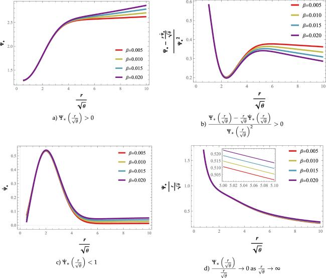
Figure 1. The graphical behavior of shape function $\Psi$* for Gaussian non-commutative geometry with ${M}_{* }=7.25,\alpha =0.45,{{ \mathcal C }}_{2}=2$ and $\tfrac{{r}_{0}}{\sqrt{\theta }}=1.6$.
Now, by substituting the A* function into (25) and (26), we get the following pressure elements:
$\begin{eqnarray}\begin{array}{l}{p}_{{{\rm{r}}}_{* }}=-\displaystyle \frac{\alpha }{32(\beta +1){\left(\beta +6\right)}^{2}\left(\tfrac{{{r}}^{18}}{{\theta }^{9}}\right)}\\ \times \left[\Space{0ex}{3em}{0ex}\displaystyle \frac{(\beta +1){M}_{* }}{{\pi }^{3/2}\alpha }\left(13\beta (\beta +6)\left(\displaystyle \frac{{{r}}^{20}}{{\theta }^{10}}\right){E}_{-\tfrac{9(\beta +1)}{\beta +6}}\left(\displaystyle \frac{{{r}}^{2}}{4\theta }\right)\right.\right.\\ \left.\,+36(\beta +1)\left(-6(2\beta -1){\left(\displaystyle \frac{{r}}{\sqrt{\theta }}\right)}^{\tfrac{90}{\beta +6}}{\left(\displaystyle \frac{{{r}}_{0}}{\sqrt{\theta }}\right)}^{\tfrac{18(\beta +1)}{\beta +6}}{E}_{\tfrac{45}{\beta +6}-8}\left(\displaystyle \frac{{{r}}_{0}^{2}}{4\theta }\right)\right.\\ \left.\,-(\beta +6)\left(\displaystyle \frac{{{r}}^{18}}{{\theta }^{9}}\right){E}_{\tfrac{45}{\beta +6}-8}\left(\displaystyle \frac{{{r}}^{2}}{4\theta }\right)\right)\right)\\ \left.\,+\displaystyle \frac{64(\beta +6)(2\beta -3)\left((\beta +6)\left(\tfrac{{{r}}^{16}}{{\theta }^{8}}\right)-9(\beta +1){\left(\tfrac{{r}}{\sqrt{\theta }}\right)}^{\tfrac{90}{\beta +6}}{\left(\tfrac{{{r}}_{0}}{\sqrt{\theta }}\right)}^{\tfrac{15\beta }{\beta +6}+1}\right)}{8\beta +3}\right],\end{array}\end{eqnarray}$
$\begin{eqnarray}\begin{array}{l}{p}_{{{\rm{t}}}_{* }}\\ =\displaystyle \frac{{M}_{* }\left(36(\beta +1){E}_{\tfrac{45}{\beta +6}-8}\left(\tfrac{{r}^{2}}{4\theta }\right)-(\beta +6)\left(\tfrac{{r}^{2}}{4\theta }\right){E}_{-\tfrac{9(\beta +1)}{\beta +6}}\left(\tfrac{{r}^{2}}{4\theta }\right)\right)}{32{\pi }^{3/2}(\beta +6)}\\ +\displaystyle \frac{\alpha }{(\beta +1)\left(\tfrac{{r}^{2}}{\theta }\right)}.\end{array}\end{eqnarray}$
In our study, the behavior of energy density and energy conditions are illustrated in figure 2. Both dominant energy conditions, radial null energy condition and strong energy condition are violated. However, the tangential null energy condition is satisfied.
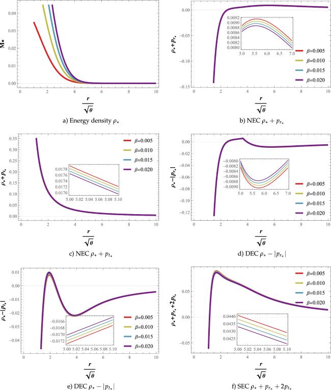
Figure 2. Gaussian Source: The profile of energy density and energy conditions with respect to $\tfrac{r}{\sqrt{\theta }}$ for different values of β with fixed parameters ${M}_{* }=7.25,\alpha =0.45,{{ \mathcal C }}_{2}=2$ and $\tfrac{{r}_{0}}{\sqrt{\theta }}=1.6$.

4.2. Lorentzian energy density

In this subsection, we focus on the scenario involving non-commutative geometry with the Lorentzian distribution. By substituting the Lorentzian energy density (28) into (24), we get
$\begin{eqnarray}\begin{array}{l}\displaystyle \frac{{M}_{* }}{{\pi }^{2}{\left(\tfrac{{r}^{2}}{\theta }+1\right)}^{2}}\\ =\displaystyle \frac{\alpha \left((\beta +6)\left(\tfrac{r}{\sqrt{\theta }}\right){\dot{A}}_{* }\left(\tfrac{r}{\sqrt{\theta }}\right)+2(8\beta +3){A}_{* }\left(\tfrac{r}{\sqrt{\theta }}\right)+2(2\beta -3){{ \mathcal C }}_{2}\right)}{6(\beta +1)(2\beta -1){{ \mathcal C }}_{2}\tfrac{{r}^{2}}{\theta }}.\end{array}\end{eqnarray}$
Solving the aforementioned differential equation while imposing the throat condition on the shape function, we can derive the following expression:
$\begin{eqnarray*}\begin{array}{l}{A}_{* }\left(\displaystyle \frac{r}{\sqrt{\theta }}\right)=\displaystyle \frac{{{ \mathcal C }}_{2}{\left(\tfrac{r}{\sqrt{\theta }}\right)}^{\tfrac{90}{\beta +6}-16}}{{\pi }^{2}\alpha (8\beta +3)}\left[3\left(2{\beta }^{2}+\beta -1\right){M}_{* }\left({\left(\displaystyle \frac{r}{\sqrt{\theta }}\right)}^{\tfrac{15\beta }{\beta +6}+1}\right.\right.\\ \,\times \left({}_{2}{F}_{1}\left(1,\displaystyle \frac{8\beta +3}{\beta +6};\displaystyle \frac{9(\beta +1)}{\beta +6};-\displaystyle \frac{{r}^{2}}{\theta }\right)\right.\\ \left.-{\,}_{2}{F}_{1}\left(2,\displaystyle \frac{8\beta +3}{\beta +6};\displaystyle \frac{9(\beta +1)}{\beta +6};-\displaystyle \frac{{r}^{2}}{\theta }\right)\right)\end{array}\end{eqnarray*}$
$\begin{eqnarray}\begin{array}{l}\,+{\left(\displaystyle \frac{{r}_{0}}{\sqrt{\theta }}\right)}^{\tfrac{15\beta }{\beta +6}+1}\left({}_{2}{F}_{1}\left(2,\displaystyle \frac{8\beta +3}{\beta +6};\displaystyle \frac{9(\beta +1)}{\beta +6};-\displaystyle \frac{{r}_{0}^{2}}{\theta }\right)\right.\\ \left.\left.{-}_{2}{F}_{1}\left(1,\displaystyle \frac{8\beta +3}{\beta +6};\displaystyle \frac{9(\beta +1)}{\beta +6};-\displaystyle \frac{{r}_{0}^{2}}{\theta }\right)\right)\right)\\ \left.-{\pi }^{2}\alpha (2\beta -3)\left({\left(\displaystyle \frac{r}{\sqrt{\theta }}\right)}^{\tfrac{15\beta }{\beta +6}+1}-{\left(\displaystyle \frac{{r}_{0}}{\sqrt{\theta }}\right)}^{\tfrac{15\beta }{\beta +6}+1}\right)\right],\end{array}\end{eqnarray}$
where 2F1(a, b; c; z) is the hypergeometric function. Hence, the resulting shape function can be expressed as follows:
$\begin{eqnarray}\begin{array}{l}{{\rm{\Psi }}}_{* }\left(\displaystyle \frac{r}{\sqrt{\theta }}\right)=\displaystyle \frac{1}{8\beta +3}\left[\displaystyle \frac{3\left(2{\beta }^{2}+\beta -1\right){M}_{* }{\left(\tfrac{r}{\sqrt{\theta }}\right)}^{-\tfrac{15\beta }{\beta +6}}}{{\pi }^{2}\alpha }\right.\\ \,\times \left({\left(\displaystyle \frac{r}{\sqrt{\theta }}\right)}^{\tfrac{15\beta }{\beta +6}+1}\left({\,}_{2}{F}_{1}\left(2,\displaystyle \frac{8\beta +3}{\beta +6};\displaystyle \frac{9(\beta +1)}{\beta +6};-\displaystyle \frac{{r}^{2}}{\theta }\right)\right.\right.\\ \left.-{\,}_{2}{F}_{1}\left(1,\displaystyle \frac{8\beta +3}{\beta +6};\displaystyle \frac{9(\beta +1)}{\beta +6};-\displaystyle \frac{{r}^{2}}{\theta }\right)\right)\\ +{\left(\displaystyle \frac{{r}_{0}}{\sqrt{\theta }}\right)}^{\tfrac{15\beta }{\beta +6}+1}\left({\,}_{2}{F}_{1}\left(1,\displaystyle \frac{8\beta +3}{\beta +6};\displaystyle \frac{9(\beta +1)}{\beta +6};-\displaystyle \frac{{r}_{0}^{2}}{\theta }\right)\right.\\ \left.\left.-{\,}_{2}{F}_{1}\left(2,\displaystyle \frac{8\beta +3}{\beta +6};\displaystyle \frac{9(\beta +1)}{\beta +6};-\displaystyle \frac{{r}_{0}^{2}}{\theta }\right)\right)\right)\\ \left.+(3-2\beta ){\left(\displaystyle \frac{r}{\sqrt{\theta }}\right)}^{-\tfrac{15\beta }{\beta +6}}{\left(\displaystyle \frac{{r}_{0}}{\sqrt{\theta }}\right)}^{\tfrac{15\beta }{\beta +6}+1}+10\beta \displaystyle \frac{r}{\sqrt{\theta }}\right],\end{array}\end{eqnarray}$
From the above expression, the derivative of the shape function is given by
$\begin{eqnarray}{\dot{{\rm{\Psi }}}}_{* }\left(\displaystyle \frac{{r}_{0}}{\sqrt{\theta }}\right)=\displaystyle \frac{5\beta -\tfrac{6\left(2{\beta }^{2}+\beta -1\right){M}_{* }\tfrac{{r}_{0}^{2}}{\theta }}{{\pi }^{2}\alpha {\left(\tfrac{{r}_{0}^{2}}{\theta }+1\right)}^{2}}}{\beta +6}.\end{eqnarray}$
Here, we will present the graphical representation of the obtained shape function as well as its criteria that must be fulfilled for the choice of the parameters ${M}_{* }=7.25,\alpha =0.4,{{ \mathcal C }}_{2}=2$ and $\tfrac{{r}_{0}}{\sqrt{\theta }}=1.6$ to analyze the results fruitfully. From figure 3(a), the positive and increased nature of shape function ${{\rm{\Psi }}}_{* }\left(\displaystyle \frac{r}{\sqrt{\theta }}\right)$ reveals that the Lorentzian distribution satisfied the wormhole geometry for conformal symmetry in the context of $f({ \mathcal Q },{ \mathcal T })$ gravity. Furthermore, the obtained shape function satisfies the flaring-out condition in figures 3(b), (c). For an infinitely large value of the radial coordinate $\displaystyle \frac{{{\rm{\Psi }}}_{* }\left(\tfrac{r}{\sqrt{\theta }}\right)}{\tfrac{r}{\sqrt{\theta }}}\to 0$ [figure 3(d)]. Therefore, we can assert that the obtained shape function fulfills all the necessary requirements of the wormhole.
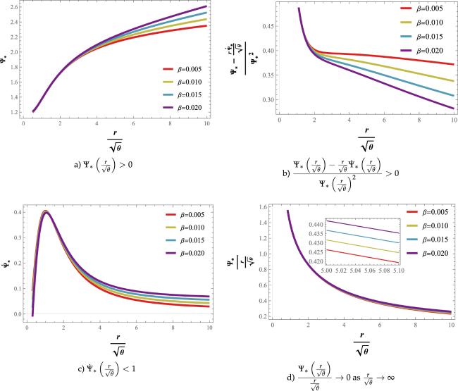
Figure 3. The graphical behavior of shape function $\Psi$* for Lorentzian non-commutative geometry with ${M}_{* }=7.25,\alpha =0.45,{{ \mathcal C }}_{2}=2$ and $\tfrac{{r}_{0}}{\sqrt{\theta }}=1.6$.
Now, substituting function (36) into (25) and (26), we get the pressure elements as
$\begin{eqnarray}\begin{array}{l}{p}_{r_{*}}=\displaystyle \frac{1}{\left(\tfrac{{{r}}^{18}}{{\theta }^{9}}\right)}\left[\displaystyle \frac{6(2\beta -1){M}_{* }{\rm{\Gamma }}\left(\tfrac{5(2\beta +3)}{\beta +6}\right)}{{\pi }^{2}(8\beta +3)}\right.\\ \times \left({\left(\displaystyle \frac{{r}}{\sqrt{\theta }}\right)}^{\tfrac{90}{\beta +6}}{\left(\displaystyle \frac{{{r}}_{0}}{\sqrt{\theta }}\right)}^{\tfrac{15\beta }{\beta +6}+1}\left({\,}_{2}{\tilde{F}}_{1}\left(2,\displaystyle \frac{8\beta +3}{\beta +6};\displaystyle \frac{9(\beta +1)}{\beta +6};-\displaystyle \frac{{{r}}_{0}^{2}}{\theta }\right)\right.\right.\\ \left.-{\,}_{2}{\tilde{F}}_{1}\left(1,\displaystyle \frac{8\beta +3}{\beta +6};\displaystyle \frac{9(\beta +1)}{\beta +6};-\displaystyle \frac{{{r}}_{0}^{2}}{\theta }\right)\right)\\ +\displaystyle \frac{{{r}}^{16}}{{\theta }^{8}}\left({\,}_{2}{\tilde{F}}_{1}\left(1,\displaystyle \frac{8\beta +3}{\beta +6};\displaystyle \frac{9(\beta +1)}{\beta +6};-\displaystyle \frac{{{r}}^{2}}{\theta }\right)\right.\\ \left.\left.\,-{\,}_{2}{\tilde{F}}_{1}\left(2,\displaystyle \frac{8\beta +3}{\beta +6};\displaystyle \frac{9(\beta +1)}{\beta +6};-\displaystyle \frac{{{r}}^{2}}{\theta }\right)\right)\right)+\displaystyle \frac{1}{\beta +6}\\ \,\times \left(\displaystyle \frac{2\alpha (2\beta -3)\left(9(\beta +1){\left(\tfrac{{r}}{\sqrt{\theta }}\right)}^{\tfrac{90}{\beta +6}}{\left(\tfrac{{{r}}_{0}}{\sqrt{\theta }}\right)}^{\tfrac{15\beta }{\beta +6}+1}-(\beta +6)\tfrac{{{r}}^{16}}{{\theta }^{8}}\right)}{(\beta +1)(8\beta +3)}\right.\\ \left.\left.-\displaystyle \frac{13\beta {M}_{* }\tfrac{{{r}}^{18}}{{\theta }^{9}}}{{\pi }^{2}{\left({x}^{2}+1\right)}^{2}}\right)\right],\end{array}\end{eqnarray}$
$\begin{eqnarray}{p}_{{{\rm{t}}}_{* }}=\displaystyle \frac{\alpha }{(\beta +1)\tfrac{{r}^{2}}{\theta }}-\displaystyle \frac{{M}_{* }}{{\pi }^{2}{\left(\tfrac{{r}^{2}}{\theta }+1\right)}^{2}}.\end{eqnarray}$
where Γ(a, z) is the gamma function.
Figure 4 illustrates the characteristics of the energy conditions and the corresponding energy density profile for Lorentzian distribution. It shows that in this scenario, the radial null energy condition [figure 4(b)] and dominant energy conditions [figure 4(d)] are violated. But, the tangential null energy condition [figure 4(c)] and strong energy condition [figure 4(f)] are obeyed.
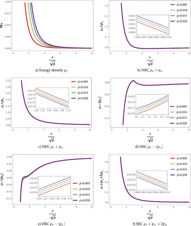
Figure 4. Lorentzian Source: The profile of energy density and energy conditions with respect to $\tfrac{r}{\sqrt{\theta }}$ for different values of β with fixed parameters ${M}_{* }=7.25,\alpha =0.45,{{ \mathcal C }}_{2}=2$ and $\tfrac{{r}_{0}}{\sqrt{\theta }}=1.6$.
Moreover, by investigating the existence of wormhole solutions and analyzing energy conditions in the late-time universe, we explore exotic matter and energy distributions that could enable the formation and stability of wormholes. The presence or absence of these solutions has significant implications for our understanding of the late-time universe’s evolution and the nature of exotic matter needed to support such structures.

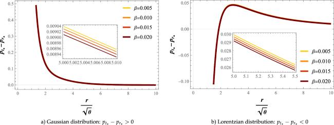
5. Effect of anisotropy

In this section, we explore the anisotropy of Gaussian and Lorentzian non-commutative geometry in order to understand the characteristics of the anisotropic pressure. The quantification of anisotropy plays a crucial role in revealing the internal geometry of a relativistic wormhole configuration. It is well known that the level of anisotropy within a wormhole can be measured using the following formula [20, 49, 62, 7173]:
$\begin{eqnarray}{\rm{\Delta }}={p}_{{{\rm{t}}}_{* }}-{p}_{{{\rm{r}}}_{* }}.\end{eqnarray}$
We can determine the geometry of the wormhole based on anisotropic factor. When the tangential pressure is greater than the radial pressure, it results in Δ > 0. This signifies that the structure of the wormhole is repulsive and anisotropic force is acting in an outward direction. Conversely, if the radial pressure is greater than the tangential pressure, it yields Δ < 0. This indicates an attractive geometry of the wormhole and force is directed inward. The anisotropy for both the Gaussian (ΔG) and Lorentzian (ΔL) distributions with the linear model is calculated as
$\begin{eqnarray}\begin{array}{l}{{\rm{\Delta }}}_{{\rm{G}}}=\displaystyle \frac{3{\left(\tfrac{r}{\sqrt{\theta }}\right)}^{-\tfrac{18(\beta +1)}{\beta +6}}}{4(\beta +1){\left(\beta +6\right)}^{2}}\left[\displaystyle \frac{4\alpha (\beta +6)\left((\beta +6)(4\beta -1){\left(\tfrac{r}{\sqrt{\theta }}\right)}^{\tfrac{16\beta +6}{\beta +6}}-6(\beta +1)(2\beta -3){\left(\tfrac{{r}_{0}}{\sqrt{\theta }}\right)}^{\tfrac{15\beta }{\beta +6}+1}\right)}{8\beta +3}\right.\\ \left.-\displaystyle \frac{9{\left(\beta +1\right)}^{2}(2\beta -1){M}_{* }{\left(\tfrac{{r}_{0}}{\sqrt{\theta }}\right)}^{\tfrac{18(\beta +1)}{\beta +6}}{E}_{\tfrac{45}{\beta +6}-8}\left(\tfrac{{r}_{0}^{2}/\theta }{4}\right)}{{\pi }^{3/2}}\right]+\displaystyle \frac{3(2\beta -1){M}_{* }\tfrac{{r}^{2}}{\theta }{E}_{-\tfrac{9(\beta +1)}{\beta +6}}\left(\tfrac{{r}^{2}/\theta }{4}\right)}{16{\pi }^{3/2}(\beta +6)},\end{array}\end{eqnarray}$
$\begin{eqnarray}\begin{array}{l}{{\rm{\Delta }}}_{{\rm{L}}}=\displaystyle \frac{\tfrac{\alpha \left(18(\beta +1)(2\beta -3){\left(\tfrac{r}{\sqrt{\theta }}\right)}^{\tfrac{90}{\beta +6}}{\left(\tfrac{{r}_{0}}{\sqrt{\theta }}\right)}^{\tfrac{15\beta }{\beta +6}+1}+(\beta +6)(4\beta +9)\tfrac{{r}^{16}}{{\theta }^{8}}\right)}{(\beta +1)(8\beta +3)\tfrac{{r}^{18}}{{\theta }^{9}}}-\tfrac{2(7\beta +3){M}_{* }}{{\pi }^{2}{\left(\tfrac{{r}^{2}}{\theta }+1\right)}^{2}}}{\beta +6}\\ +\displaystyle \frac{6(2\beta -1){M}_{* }{\rm{\Gamma }}\left(\tfrac{5(2\beta +3)}{\beta +6}\right)}{{\pi }^{2}(8\beta +3)\tfrac{{r}^{18}}{{\theta }^{9}}}\left[\displaystyle \frac{{r}^{16}}{{\theta }^{8}}\left({\,}_{2}{\tilde{F}}_{1}\left(1,\displaystyle \frac{8\beta +3}{\beta +6};\displaystyle \frac{9(\beta +1)}{\beta +6};-\displaystyle \frac{{r}^{2}}{\theta }\right)\right.\right.\\ \left.-{\,}_{2}{\tilde{F}}_{1}\left(2,\displaystyle \frac{8\beta +3}{\beta +6};\displaystyle \frac{9(\beta +1)}{\beta +6};-\displaystyle \frac{{r}^{2}}{\theta }\right)\right)\\ +{\left(\displaystyle \frac{r}{\sqrt{\theta }}\right)}^{\tfrac{90}{\beta +6}}{\left(\displaystyle \frac{{r}_{0}}{\sqrt{\theta }}\right)}^{\tfrac{15\beta }{\beta +6}+1}\left({\,}_{2}{\tilde{F}}_{1}\left(2,\displaystyle \frac{8\beta +3}{\beta +6};\displaystyle \frac{9(\beta +1)}{\beta +6};-\displaystyle \frac{{r}_{0}^{2}}{\theta }\right)\right.\\ \left.\left.-{\,}_{2}{\tilde{F}}_{1}\left(1,\displaystyle \frac{8\beta +3}{\beta +6};\displaystyle \frac{9(\beta +1)}{\beta +6};-\displaystyle \frac{{r}_{0}^{2}}{\theta }\right)\right)\right].\end{array}\end{eqnarray}$
Figure 5 depicts the effect of anisotropy for a viable wormhole model under Gaussian and Lorentzian distributions. The investigation reveals that our anisotropy factor Δ is positive (i.e., ${p}_{{{\rm{t}}}_{* }}\gt {p}_{{{\rm{r}}}_{* }}$) and the structure of the wormhole is repulsive in Gaussian distribution [figure 5(a)], whereas Δ is negative (i.e., ${p}_{{{\rm{t}}}_{* }}\lt {p}_{{{\rm{r}}}_{* }}$) which indicates an attractive geometry of the wormhole in Lorentzian distribution [figure 5(b)].
Figure 5. The graphical representation of anisotropy for both distributions.

6. Results and concluding remarks

In this article, we have explored the conformal symmetric wormhole solutions under non-commutative geometry in the background of $f({ \mathcal Q },{ \mathcal T })$ gravity. To achieve this, we have considered the presence of an anisotropic fluid in a spherically symmetric space-time. The concept of conformal symmetry and non-commutative geometry have already been used in literature within various contexts of modified theories of gravity [5060, 6264]. Non-commutative geometry is used to replace the particle-like structure to smeared objects in string theory. Furthermore, conformal killing vectors are derived from the killing equation, which is based on the Lie algebra. These vectors are used to reduce the nonlinearity order of the field equation. Conformal symmetry has proved to be effective in describing relativistic stellar-type objects. Furthermore, it has led to new solutions and provided insights into geometry and kinematics [74]. It influences the geometry and dynamics of the space-time, impacting key parameters such as throat size and stability.
In the framework of extended symmetric teleparallel gravity, we have derived some new exact solutions for wormholes by using both Gaussian and Lorentzian energy densities of non-commutative geometry. For this object, we presumed the linear wormhole model as $f({ \mathcal Q },{ \mathcal T })\,=\alpha { \mathcal Q }+\beta { \mathcal T }$, where α and β are model parameters. In both cases, we examined the wormhole scenario using Gaussian and Lorentzian distributions. By applying the throat condition in two distributions, we obtained different shape functions that obey all the criteria for a traversable wormhole. A similar result was presented in [63] where the authors explored wormhole solutions in curvature-matter coupling gravity supported by non-commutative geometry and conformal symmetry. Furthermore, we investigated the impact of model parameters on these two shape functions. Due to the conformal symmetry, the redshift function does not approach zero as r > r0 [8, 59, 60, 75].
Figures 1 and 3 show the graphical nature of the obtained shape functions with β ∈ [0, 0.5). Notably, a slight variation in the value of β can impact the nature of the shape function. Moreover, the graphical behavior of the energy conditions is shown in figures 2 and 4. The energy density is positive throughout the space-time. For all the wormhole solutions, the violation of the null energy conditions indicates the presence of hypothetical matter. Here, this nature of hypothetical fluid is presented in references [63, 76, 77]. Next, we studied the effect of anisotropy for both distributions. The geometry of the wormhole is repulsive in the Gaussian distribution, whereas it is attractive in the Lorentzian distribution [figure 5].
To conclude, this work validates the conformal symmetric wormhole solutions in $f({ \mathcal Q },{ \mathcal T })$ gravity under non-commutative geometry. The authors [78] have identified the possibility of a generalized wormhole formation in the galactic halo due to dark matter using observational data within the matter coupling gravity formalism. In the near future, we plan to investigate various wormhole scenarios in alternative theories of gravity, as discussed in references [7982].

CCC, VV and NSK acknowledge DST, New Delhi, India, for its financial support for research facilities under DST-FIST-2019.

1
Flamm L 1916 Beiträge zur Einsteinschen Gravitationstheorie Phys. Z 17 448

2
Einstein A Rosen N 1935 The particle problem in the general theory of relativity Phys. Rev. 48 73

DOI

3
Morris M S Thorne K S 1988 Wormholes in space-time and their use for interstellar travel: a tool for teaching general relativity AJP 6 395

DOI

4
González-Díaz P F 2003 Wormholes and ringholes in a dark-energy universe Phys. Rev. D 68 084016

DOI

5
Armendáriz-Picón C 2002 On a class of stable, traversable Lorentzian wormholes in classical general relativity Phys. Rev. D 65 104010

DOI

6
Visser M 1989 Traversable wormholes from surgically modified Schwarzschild space-times Nuclear Phys. B 328 203

DOI

7
Visser M 1989 Traversable wormholes: some simple examples Phys. Rev. D 39 3182

DOI

8
Kuhfittig P K F 1999 A wormhole with a special shape function Am. J. Phys. 67 125

DOI

9
Lobo F S N Oliveira M A 2009 Wormhole geometries in f(R) modified theories of gravity Phys. Rev. D 80 104012

DOI

10
Azizi T 2013 Wormhole Geometries in f(R, T) Gravity Int. J. Theor. Physc. 52 3486 3493

DOI

11
Böhmer C G Harko T Lobo F S N 2012 Wormhole geometries in modified teleparallel gravity and the energy conditions Phys. Rev. D 85 044033

DOI

12
Sharif M Rani S 2013 Wormhole solutions in f(T) gravity with noncommutative geometry Phys. Rev. D 88 123501

DOI

13
Singh K N 2020 Conformally symmetric traversable wormholes in modified teleparallel gravity Phys. Rev. D 101 084012

DOI

14
Jiménez J B Heisenberg L Koivisto T 2018 Coincident general relativity Phys. Rev. D 98 044048

DOI

15
Yixin X 2019 f(Q, T) gravity Eur. Phys. J. C 79 708

DOI

16
Rahaman F 2006 A theoretical construction of wormhole supported by phantom energy Phys. Lett. B 633 2 3

DOI

17
Zubair M Waheed S Ahmad Y 2016 Static spherically symmetric wormholes in f(R, T) gravity Eur. Phys. J. C 76 444

DOI

18
Maldacena J Milekhin A Popov F 2020 Traversable wormholes in four dimensions arXiv:1807.04726v3

19
Övgün A 2018 Light deflection by Damour-Solodukhin wormholes and Gauss-Bonnet theorem Phys. Rev. D 98 044033

DOI

20
Mustafa G 2021 Traversable wormholes in the extended teleparallel theory of gravity with matter coupling Fortschr. Phys. 69 2100048

DOI

21
Elizalde E Khurshudyan M 2019 Wormhole models in f(R, T) gravity Int. J. Mod. Phys. D 28 1950172

DOI

22
Anchordoqui L A Bergliaffa S E P 2000 Wormhole surgery and cosmology on the brane: the world is not enough Phys. Rev. D 62 067502

DOI

23
Lobo F S N Simpson A Visser M 2020 Dynamic thin-shell black-bounce traversable wormholes Phys. Rev. D 101 124035

DOI

24
Capozziello S Luongo O Mauro L 2021 Traversable wormholes with vanishing sound speed in f(R) gravity Eur. Phys. J. Plus 136 167

DOI

25
Capozziello S Godani Nisha 2022 Non-local gravity wormholes Phys. Lett. B 835 137572

DOI

26
Venkatesha V 2023 Wormhole geometry and three-dimensional embedding in extended symmetric teleparallel gravity New Astron. 105 102090

DOI

27
Naz T 2023 Evolving embedded traversable wormholes in f(R, G) gravity: a comparative study Phys. Dark Universe 42 101301

DOI

28
Malik A 2023 Investigation of traversable wormhole solutions in modified f(R) gravity with scalar potential Eur. Phys. J. C 83 522

DOI

29
Venkatesha V Kavya N S Sahoo P K 2023 Geometric structures of Morris-Thorne wormhole metric in f(R, Lm) gravity and energy conditions Phys. Scr. 98 065020

DOI

30
Malik A 2023 Embedding procedure and wormhole solutions in Rastall gravity utilizing the class I approach Int. J. of Geometric Methods Mod. Phys. 20 2350145

DOI

31
Malik A 2022 Traversable wormhole solutions in theories of gravity Via Karmarkar condition Chin. Phys. C 46 095104

DOI

32
Kavya N S 2023 Static traversable wormhole solutions in f(R, Lm) gravity Chin. J. Phys. 84 1 11

DOI

33
Malik A Nafees A 2021 Existence of Static Wormhole Solutions in Gravity New Astron. 89 101632

DOI

34
Shamir M F Malik A Mustafa G 2021 Wormhole Solutions in f(R, φ, X) Modified f(R, φ, X) Gravity Int. J. Mod. Phys. A 36 2150021

DOI

35
Zubair M 2017 Existence of stable wormholes on a non-commutative-geometric background in modified gravity Eur. Phys. J. C 77 1 13

DOI

36
Mustafa G Hussain I Shamir M F 2020 Stable wormholes in the background of an exponential f(R) gravity Universe 6 48

DOI

37
Doplicher S Fredenhagen K Roberts J E 1994 Space-time quantization induced by classical gravity Phys. Lett. B 331 39

DOI

38
Witten E 1996 Bound states of strings and p-branes Nucl. Phys. B 460 335

DOI

39
Seiberg N Witten E 1999 String theory and noncommutative geometry J. High Energy Phys. 09 JHEP09(1999)032

DOI

40
Kase H 2003 Lorentz-invariant non-commutative space-time based on DFR algebra Prog. Theor. Phys. 109 663

DOI

41
Smailagic A Spallucci E 2004 Lorentz invariance, unitarity and UV-finiteness of QFT on noncommutative space-time J. Phys. A 37 1

DOI

42
Nicolini P 2009 Noncommutative black holes, the final appeal to quantum gravity: a review Int. J. Mod. Phys. A 24 1229

DOI

43
Jamil M 2014 Nonommutative wormholes in f(R) gravity J. Korean Phys. Soc. 65 917

DOI

44
Rahaman F 2015 Fluid sphere: stability problem and dimensional constraint Int. J. Mod. Phys. D 24 1550049

DOI

45
Rahaman F 2014 Noncommutative wormholes in f(R) gravity with Lorentzian distribution Int. J. Theor. Phys. 53 1910 1919

DOI

46
Rahaman F 2012 Searching for higher-dimensional wormholes with noncommutative geometry Phys. Rev. D 86 106010

DOI

47
Zubair M 2019 Noncommutative inspired wormholes admitting conformal motion involving minimal coupling Int. J. Mod. Phys. D 28 1950067

DOI

48
Khufittig P K F 2016 Stable wormholes on a noncommutative-geometry background admitting a one-parameter group of conformal motions Indian J. Phys. 90 837 842

DOI

49
Shamir M F Malik A Mustafa G 2021 Noncommutative wormhole solutions in modified f(R) theory of gravity Chinese J. Phys. 73 634 648

DOI

50
Aschieri P 2006 Noncommutative geometry and gravity Class. Quant. Grav. 23 1883

DOI

51
Schneider M DeBenedictis A 2020 Noncommutative black holes of various genera in the connection formalism Phys. Rev. D 102 024030

DOI

52
Sushkov S 2005 Wormholes supported by a phantom energy Phys. Rev. D 71 043520

DOI

53
Kuhfittig P K F 2012 On the stability of thin-shell wormholes in noncommutative geometry Advances in High Energy Phys. 2012 462493

DOI

54
Lobo F S N Garattini R 2013 Linearized stability analysis of gravastars in noncommutative geometry J. High Energy Phys. JHEP12(2013)065

DOI

55
Nicolini P Spalluci E 2009 Noncommutative geometry-inspired dirty black holes Class. Quant. Grav. 27 015010

DOI

56
Kuhfittig P K F 2023 Macroscopic noncommutative-geometry wormholes as emergent phenomena Lett. High Energy Phys. 2023 3999

DOI

57
Kuhfittig P K F 2023 Noncommutative-geometry wormholes based on the Casimir effect JHEP Grav. Cosmol. 9 295

DOI

58
Smailagic A Spalluci E 2003 Feynman path integral on the non-commutative plane J. Phys. A Math. Gen. 36 L467

DOI

59
Rahaman F 2015 Wormhole inspired by non-commutative geometry Phys. Lett. B 746 73

DOI

60
Rahaman F 2015 Noncommutative geometry inspired wormholes with conformal motion Int. J. Theor. Phys. 54 699

DOI

61
Mustafa G Abbas G Xia T 2019 Wormhole solutions in F(T, TG) gravity under Gaussian and Lorentzian non-commutative distributions with conformal motions Chin. J. Phys. 60 362 378

DOI

62
Hassan Z Mustafa G Sahoo P K 2021 Wormhole solutions in symmetric teleparallel gravity with noncommutative geometry Symmetry 13 1260

DOI

63
Kavya N S Mustafa G Venkatesha V Sahoo P K 2024 Exploring wormhole solutions in curvature-matter coupling gravity supported by noncommutative geometry and conformal symmetry Chin. J. Phys. 87 751 765

DOI

64
Kavya N S 2023 On possible wormhole solutions supported by non-commutative geometry within f(R, Lm) gravity Ann. Phys. 455 169383

DOI

65
Bhattacharjee S Sahoo P K 2020 Baryogenesis in f(Q, T) gravity Eur. Phys. J. C 80 289

DOI

66
Arora S 2020 f(Q, T) gravity models with observational constraints Phys. Dark Univ. 30 100664

DOI

67
Chalavadi C C Kavya N S Venkatesha V 2023 Wormhole solutions supported by non-commutative geometric background in f(Q, T) gravity Eur. Phys. J. Plus 138 1 14

DOI

68
Mustafa G 2020 Non-commutative wormholes exhibiting conformal motion in Rastall gravity Chinese J. Phys. 65 163 176

DOI

69
Böhmer C G Harko T Lobo F S 2008 Wormhole geometries with conformal motions Class. Quantum Grav. 7 075016

DOI

70
Nicolini P Smailagic A Spallucci E 2006 Noncommutative geometry inspired Schwarzschild black hole Phys. Lett. B 632 547 551

DOI

71
Rahaman F Kalam M Rahman K A 2009 Wormhole geometry from real feasible matter sources Int. J. Theor. Phys. 48 471 475

DOI

72
Sharif M Saba S 2018 Gravitational decoupled anisotropic solutions in f(G) gravity Eur. Phys. J. C 78 921

DOI

73
Shamir M F Asghar Z Malik A 2022 Relativistic Krori-Barua compact stars in f(R, T)f(R, T) gravity Fortschr. Phys. 70 2200134

DOI

74
Kuhfittig P K F 2015 Wormholes with a barotropic equation of state admitting a one-parameter group of conformal motions Annals Phys. 355 115 120

DOI

75
Mustafa G 2020 Stable wormholes solutions in the background of Rastall theory Mod. Phys. Lett. A 35 2050035

DOI

76
Mustafa G Hassan Z Sahoo P K 2022 Traversable wormhole inspired by non-commutative geometries in f(Q) gravity with conformal symmetry Annals Phys. 437 168751

DOI

77
Mustafa G 2020 Noncommutative wormholes solutions with conformal motion in the background of f(G, T) gravity Int. J. Geometric Methods Mod. Phys. 17 2050103

DOI

78
Mustafa G Maurya S K Ray S 2022 On the possibility of generalized wormhole formation in the galactic halo due to dark matter using the observational data within the matter coupling gravity formalism Astrophys. J. 941 170

DOI

79
Ditta A 2021 A study of traversable wormhole solutions in extended teleparallel theory of gravity with matter coupling Eur. Phys. J. C 81 880

DOI

80
Mustafa G Atamurotov F Ghosh S G 2023 Structural properties of generalized embedded wormhole solutions via dark matter halos in Einsteinian-cubic-gravity with quasi-periodic oscillations Phys. Dark Universe 40 101214

DOI

81
Mustafa G Maurya S K Ray S 2023 Relativistic wormhole surrounded by dark matter halos in symmetric teleparallel gravity Fortschr. Phys. 71 2200129

DOI

82
Mustafa G 2023 New wormhole model with quasi-periodic oscillations exhibiting conformal motion in $f({ \mathcal T },T)$ gravity Commun. Theor. Phys. 75 095201

DOI

Outlines

/