


1. Introduction
2. Planar collections of Feynman diagrams

Figure 1. An example for an initial planar collection obtained by pruning a six-point Feynman diagram. Above is the six-point Feynman diagram to be pruned. Below is the planar collection of five-point Feynman diagrams obtained by pruning the leaves 1, 2, ⋯, 6 of the above Feynman diagram, respectively. |
Table 1. Summary of results for planar collections of Feynman diagrams for k = 3 and up to n = 9. The second column gives the total number of planar collections. The third column provides the number of collections for each kind, classified by the number of mutations. The fourth column indicates how many layers of mutations are necessary to find the complete set of collections starting with the Cn−2 initial collections. |
| (k, n) | Number of collections | Numbers of collections for each kind | Number of layers | ||||
|---|---|---|---|---|---|---|---|
| (3, 5) | 5 | 2-mut. | 0 | ||||
| 5 | |||||||
| (3, 6) | 48 | 4-mut. | 6-mut. | 3 | |||
| 46 | 2 | ||||||
| (3, 7) | 693 | 6-mut. | 7-mut. | 8-mut. | 4 | ||
| 595 | 28 | 70 | |||||
| (3, 8) | 13 612 | 8-mut. | 9-mut. | 10-mut. | 11-mut. | 12-mut. | 8 |
| 9 672 | 1 488 | 2 280 | 96 | 76 | |||
| (3, 9) | 346 710 | 10-mut. | 11-mut. | 12-mut. | 13-mut. | 14-mut. | 11 |
| 186 147 | 61 398 | 78 402 | 12 300 | 7 668 | |||
| 15-mut. | 16-mut. | 17-mut. | |||||
| 522 | 270 | 3 | |||||
3. Planar matrices of Feynman diagrams
A planar matrix of Feynman diagrams is an n × n matrix ${ \mathcal M }$ with component ${{ \mathcal M }}_{{ij}}$ given by a metric tree with leaves $\{1,2,\ldots ,n\}\setminus \{i,j\}$ and planar with respect to the ordering $(1,2,\cdots ,\rlap{/}{i},\cdots ,\rlap{/}{j},\cdots ,n)$ satisfying the following conditions:
| • | diagonal entries are the empty tree ${{ \mathcal M }}_{{ii}}=\varnothing $ |
| • | compatibility ( $\begin{eqnarray*}{d}_{{kl}}^{({ij})}={d}_{{jl}}^{({ik})}={d}_{{kj}}^{({il})}={d}_{{ij}}^{({kl})}={d}_{{ik}}^{({jl})}={d}_{{il}}^{({kj})}.\end{eqnarray*}$ |
Planar matrices of Feynman diagrams are symmetric.
The symmetry of the matrix follows from realizing that the compatibility condition requires that ${d}_{{kl}}^{({ij})}={d}_{{ij}}^{({kl})}$ and therefore the symmetry of the metric on the left-hand side in the leave labels k and l implies that of the right-hand side is symmetric in the matrix labels k and l. In order to complete the proof, it is enough to note that a binary metric tree is uniquely determined by its metric, as we show in appendix
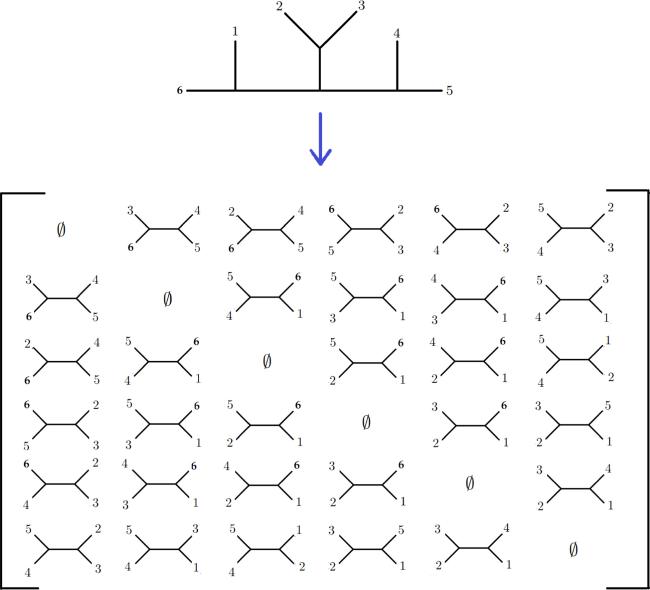
Figure 2. An example of a six-point initial planar matrix. Above we show a six-point Feynman diagram. Below there is a symmetric matrix of four-point Feynman diagrams obtained by pruning two leaves at a time from the set 1, 2, ⋯, 6 of the above Feynman diagram. The Feynman diagram from the ith column and jth row has the ith and jth leaves pruned. |
3.1. Second combinatorial bootstrap
Table 2. Number of planar matrices of Feynman diagrams and number of degenerate matrices for different values of n. |
| (4, 6) | (4, 7) | (4, 8) | (4, 9) | |
|---|---|---|---|---|
| Planar matrices | 14 | 693 | 90 608 | 30 659 424 |
| Degenerate matrices | 0 | 0 | 888 | 2 523 339 |
3.2. A simple example: from (3,5) to (4,6)

Figure 3. The five k = 2 planar Feynman diagrams and their corresponding collections in (k, n) = (3, 5). |
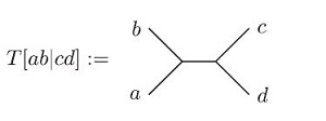
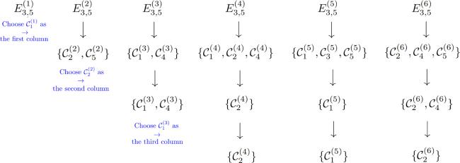
Figure 4. Illustration of the second combinatorial bootstrap for obtaining planar matrices of Feynman diagrams. Here we choose ${{ \mathcal C }}_{1}^{(1)}$, ${{ \mathcal C }}_{2}^{(2)}$ and ${{ \mathcal C }}_{1}^{(3)}$ as the first three columns and then get a symmetric planar matrix by filling in the remaining three columns with ${{ \mathcal C }}_{2}^{(4)}$, ${{ \mathcal C }}_{1}^{(5)}$ and ${{ \mathcal C }}_{2}^{(6)}$. See also table 3. |
Table 3. Planar matrices of Feynman diagrams in (4, 6). Here we abbreviate $[{{ \mathcal C }}_{{i}_{1}}^{(1)},{{ \mathcal C }}_{{i}_{2}}^{(2)},\cdots ,{{ \mathcal C }}_{{i}_{6}}^{(6)}]$ as $[{{ \mathcal C }}_{{i}_{1}},{{ \mathcal C }}_{{i}_{2}},\cdots ,{{ \mathcal C }}_{{i}_{6}}]$ since the superscripts can be inferred from the position of ${{ \mathcal C }}_{i}$ in the brackets. |
| Matrix | Collections | Matrix | Collections |
|---|---|---|---|
| ${{ \mathcal M }}_{1}$ | $[{{ \mathcal C }}_{1},{{ \mathcal C }}_{2},{{ \mathcal C }}_{1},{{ \mathcal C }}_{2},{{ \mathcal C }}_{1},{{ \mathcal C }}_{2}]$ | ${{ \mathcal M }}_{8}$ | $[{{ \mathcal C }}_{3},{{ \mathcal C }}_{2},{{ \mathcal C }}_{1},{{ \mathcal C }}_{5},{{ \mathcal C }}_{4},{{ \mathcal C }}_{4}]$ |
| ${{ \mathcal M }}_{2}$ | $[{{ \mathcal C }}_{1},{{ \mathcal C }}_{5},{{ \mathcal C }}_{4},{{ \mathcal C }}_{4},{{ \mathcal C }}_{3},{{ \mathcal C }}_{2}]$ | ${{ \mathcal M }}_{9}$ | $[{{ \mathcal C }}_{4},{{ \mathcal C }}_{4},{{ \mathcal C }}_{3},{{ \mathcal C }}_{2},{{ \mathcal C }}_{1},{{ \mathcal C }}_{5}]$ |
| ${{ \mathcal M }}_{3}$ | $[{{ \mathcal C }}_{1},{{ \mathcal C }}_{5},{{ \mathcal C }}_{4},{{ \mathcal C }}_{1},{{ \mathcal C }}_{5},{{ \mathcal C }}_{4}]$ | ${{ \mathcal M }}_{10}$ | $[{{ \mathcal C }}_{4},{{ \mathcal C }}_{1},{{ \mathcal C }}_{5},{{ \mathcal C }}_{4},{{ \mathcal C }}_{1},{{ \mathcal C }}_{5}]$ |
| ${{ \mathcal M }}_{4}$ | $[{{ \mathcal C }}_{2},{{ \mathcal C }}_{4},{{ \mathcal C }}_{3},{{ \mathcal C }}_{2},{{ \mathcal C }}_{4},{{ \mathcal C }}_{3}]$ | ${{ \mathcal M }}_{11}$ | $[{{ \mathcal C }}_{4},{{ \mathcal C }}_{3},{{ \mathcal C }}_{2},{{ \mathcal C }}_{4},{{ \mathcal C }}_{3},{{ \mathcal C }}_{2}]$ |
| ${{ \mathcal M }}_{5}$ | $[{{ \mathcal C }}_{2},{{ \mathcal C }}_{1},{{ \mathcal C }}_{5},{{ \mathcal C }}_{4},{{ \mathcal C }}_{4},{{ \mathcal C }}_{3}]$ | ${{ \mathcal M }}_{12}$ | $[{{ \mathcal C }}_{4},{{ \mathcal C }}_{3},{{ \mathcal C }}_{2},{{ \mathcal C }}_{1},{{ \mathcal C }}_{5},{{ \mathcal C }}_{4}]$ |
| ${{ \mathcal M }}_{6}$ | $[{{ \mathcal C }}_{2},{{ \mathcal C }}_{1},{{ \mathcal C }}_{2},{{ \mathcal C }}_{1},{{ \mathcal C }}_{2},{{ \mathcal C }}_{1}]$ | ${{ \mathcal M }}_{13}$ | $[{{ \mathcal C }}_{5},{{ \mathcal C }}_{4},{{ \mathcal C }}_{4},{{ \mathcal C }}_{3},{{ \mathcal C }}_{2},{{ \mathcal C }}_{1}]$ |
| ${{ \mathcal M }}_{7}$ | $[{{ \mathcal C }}_{3},{{ \mathcal C }}_{2},{{ \mathcal C }}_{4},{{ \mathcal C }}_{3},{{ \mathcal C }}_{2},{{ \mathcal C }}_{4}]$ | ${{ \mathcal M }}_{14}$ | $[{{ \mathcal C }}_{5},{{ \mathcal C }}_{4},{{ \mathcal C }}_{1},{{ \mathcal C }}_{5},{{ \mathcal C }}_{4},{{ \mathcal C }}_{1}]$ |
3.3. A more interesting example: from (3, 6) to (4, 7)
Table 4. All 48 planar collections of trees for n = 6 in a compact notation tailored to this case and explained in the text. |
| Planar collections of trees in k = 3 and n = 6 | |||
|---|---|---|---|
| Collection | Trees | Collection | Trees |
| ${{ \mathcal C }}_{1}$ | [4, 4, 4, 3, 3, 3] | ${{ \mathcal C }}_{25}$ | [6, 6, 6, 5, 4, 1] |
| ${{ \mathcal C }}_{2}$ | [4, 4, 4, 3, 6, 5] | ${{ \mathcal C }}_{26}$ | [6, 6, 6, 6, 6, 3] |
| ${{ \mathcal C }}_{3}$ | [4, 4, 4, 3, 2, 2] | ${{ \mathcal C }}_{27}$ | [6, 6, 6, 1, 1, 1] |
| ${{ \mathcal C }}_{4}$ | [4, 4, 4, 1, 4, 4] | ${{ \mathcal C }}_{28}$ | [6, 6, 6, 2, 2, 1] |
| ${{ \mathcal C }}_{5}$ | [4, 4, 4, 1, 1, 1] | ${{ \mathcal C }}_{29}$ | [6, 3, 2, 5, 4, 1] |
| ${{ \mathcal C }}_{6}$ | [4, 4, 6, 6, 6, 5] | ${{ \mathcal C }}_{30}$ | [6, 3, 2, 1, 1, 1] |
| ${{ \mathcal C }}_{7}$ | [4, 4, 6, 6, 2, 2] | ${{ \mathcal C }}_{31}$ | [6, 3, 2, 2, 2, 1] |
| ${{ \mathcal C }}_{8}$ | [4, 5, 5, 5, 4, 4] | ${{ \mathcal C }}_{32}$ | [2, 5, 5, 5, 2, 2] |
| ${{ \mathcal C }}_{9}$ | [4, 6, 6, 5, 4, 4] | ${{ \mathcal C }}_{33}$ | [2, 5, 2, 2, 2, 2] |
| ${{ \mathcal C }}_{10}$ | [4, 6, 6, 2, 2, 4] | ${{ \mathcal C }}_{34}$ | [2, 1, 4, 3, 3, 3] |
| ${{ \mathcal C }}_{11}$ | [4, 1, 1, 1, 4, 4] | ${{ \mathcal C }}_{35}$ | [2, 1, 4, 3, 6, 5] |
| ${{ \mathcal C }}_{12}$ | [4, 1, 1, 1, 1, 1] | ${{ \mathcal C }}_{36}$ | [2, 1, 4, 3, 2, 2] |
| ${{ \mathcal C }}_{13}$ | [4, 3, 2, 5, 4, 4] | ${{ \mathcal C }}_{37}$ | [2, 1, 6, 6, 6, 5] |
| ${{ \mathcal C }}_{14}$ | [4, 3, 2, 2, 2, 4] | ${{ \mathcal C }}_{38}$ | [2, 1, 6, 6, 2, 2] |
| ${{ \mathcal C }}_{15}$ | [5, 5, 4, 3, 3, 3] | ${{ \mathcal C }}_{39}$ | [2, 1, 1, 1, 3, 3] |
| ${{ \mathcal C }}_{16}$ | [5, 5, 4, 3, 6, 5] | ${{ \mathcal C }}_{40}$ | [2, 1, 1, 1, 6, 5] |
| ${{ \mathcal C }}_{17}$ | [5, 5, 5, 5, 2, 5] | ${{ \mathcal C }}_{41}$ | [2, 1, 1, 1, 2, 2] |
| ${{ \mathcal C }}_{18}$ | [5, 5, 6, 6, 6, 5] | ${{ \mathcal C }}_{42}$ | [3, 5, 5, 5, 4, 3] |
| ${{ \mathcal C }}_{19}$ | [5, 5, 1, 1, 3, 3] | ${{ \mathcal C }}_{43}$ | [3, 5, 5, 1, 1, 3] |
| ${{ \mathcal C }}_{20}$ | [5, 5, 1, 1, 6, 5] | ${{ \mathcal C }}_{44}$ | [3, 3, 6, 3, 3, 3] |
| ${{ \mathcal C }}_{21}$ | [5, 5, 2, 2, 2, 5] | ${{ \mathcal C }}_{45}$ | [3, 3, 6, 6, 6, 3] |
| ${{ \mathcal C }}_{22}$ | [6, 5, 5, 5, 4, 1] | ${{ \mathcal C }}_{46}$ | [3, 3, 2, 5, 4, 3] |
| ${{ \mathcal C }}_{23}$ | [6, 5, 5, 1, 1, 1] | ${{ \mathcal C }}_{47}$ | [3, 3, 2, 1, 1, 3] |
| ${{ \mathcal C }}_{24}$ | [6, 6, 6, 3, 3, 3] | ${{ \mathcal C }}_{48}$ | [3, 3, 2, 2, 2, 3] |
4. Main results
4.1. Planar collections of feynman diagrams
4.2. Planar matrices of feynman diagrams
5. Evaluation: computing volumes from planar collections and matrices

Figure 5. Bipyramidal collection for (3, 6). |
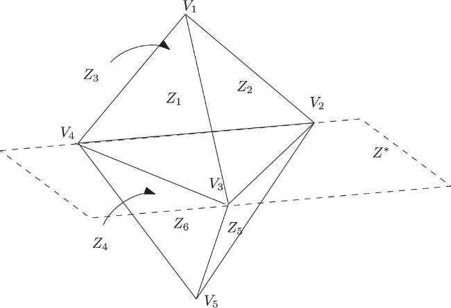
Figure 6. Bipyramid projected into a three-dimensional slice, for instance by imposing F · T = 1. Three or more planes Zi intersect at vertices Vi. We have also depicted the auxiliary plane Z* passing through V2, V3, V4. |
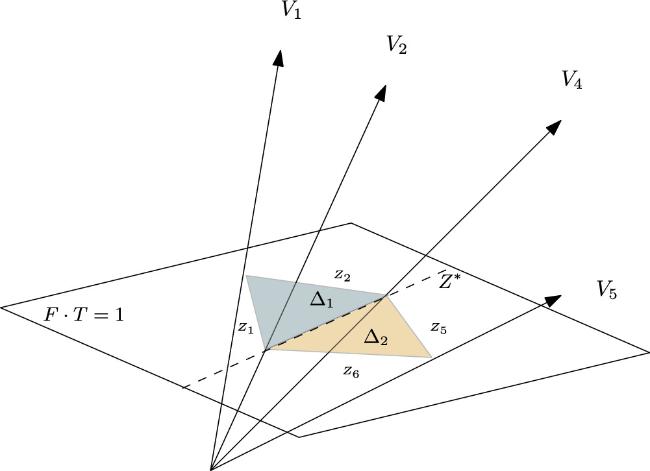
Figure 7. An illustration of the bipyramid as a cone in ${{\mathbb{R}}}^{4}$, bound by planes Zi. The vertices Vi correspond to rays. |
6. Higher k or planar arrays of Feynman diagrams and duality
A planar array of Feynman diagrams is a $(k-2)$-dimensional array ${ \mathcal A }$ with dimensions of size n. The array has as component ${{ \mathcal A }}_{{i}_{1},{i}_{2},\ldots ,{i}_{k-2}}$ a metric tree with leaves in the set $\{1,2,\ldots ,n\}\setminus \{{i}_{1},{i}_{2},\ldots ,{i}_{k-2}\}$ and which is planar with respect to the ordering $(1,2,\cdots ,{\rlap{/}{i}}_{1},\cdots ,{\rlap{/}{i}}_{2},\cdots ,{\rlap{/}{i}}_{k-2},\cdots ,n)$ satisfying the following conditions:
| • | diagonal entries are the empty tree ${{ \mathcal A }}_{\ldots ,i,\ldots ,i,\ldots }=\varnothing $ |
| • | compatibility: ${d}_{{i}_{1}{i}_{2}}^{({i}_{3},\ldots ,{i}_{k})}$ is completely symmetric in all k indices. |
6.1. Combinatorial duality
6.1.1. Illustrative example: (3, 7) ∼ (4, 7)
7. Future directions
Acknowledgments
Appendix A. Proof of one-to-one map of a binary tree and its metric
Given that two cubic trees TA and TB have the same valid non-degenerate metric dij, then TA = TB.
We are going to provide a proof by induction. First, consider the base case where TA and TB are three-point trees. It is clear that there exists a unique solution to ${d}_{12}={e}_{1}+{e}_{2}$, ${d}_{13}={e}_{1}+{e}_{3}$ and ${d}_{23}={e}_{2}+{e}_{3}$. Since TA and TB have the same non-degenerate metric, the lengths ${e}_{i}^{(A)}={e}_{i}^{(B)}$ must be identical, thus TA=TB.
Now let us assume that the lemma is true for all $(n-1)$-point cubic metric trees and consider two n-point cubic trees TA and TB that have the same non-degenerate metric dij. Next let us find leaves i and j such that ${d}_{{il}}-{d}_{{jl}}$ is l independent. Such a pair must exist because the condition is true for any pair of leaves that belong to the same 'cherry' as shown in the diagrams in figure 8. Moreover, only leaves in cherries satisfy this condition in a cubic non-degenerate tree.
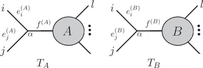
Figure 8. Two n-point cubic trees with pairs i and j joined by the vertex α. |
Removing the cherries from both trees and introducing a new leaf α one can define a metric for the the $(n-1)$-point cubic trees in figure 9, whose leaves are given by $\left(\{1,2,\ldots ,n\}\setminus \{i,j\}\right)\cup \{\alpha \}$.

Figure 9. Two (n − 1)-point cubic trees with external edges ${e}_{\alpha }^{(A)}={f}^{(A)}$ and ${e}_{\alpha }^{(B)}={f}^{(B)}$ such that ${d}_{{kl}}^{(A)}={d}_{{kl}}^{(B)}$. |
Such a metric is defined in terms of the metric of the parent trees as follows: ${d}_{{kl}}^{(A)}={d}_{{kl}}$ if $k,l\ne \alpha $ and ${d}_{k\alpha }^{(A)}={d}_{{ki}}-{e}_{i}^{(A)}$. Likewise ${d}_{{kl}}^{(B)}={d}_{{kl}}$ if $k,l\ne \alpha $ and ${d}_{k\alpha }^{(B)}={d}_{{ki}}-{e}_{i}^{(B)}$. It is easy to see from the figure that the two metrics are identical, i.e. ${d}_{{kl}}^{(A)}={d}_{{kl}}^{(B)}$.
Using the induction hypothesis, the two metric trees in figure 9 must be the same. In order to complete the proof all we need is to show that ${e}_{i}^{(A)}={e}_{i}^{(B)}$ and ${e}_{j}^{(A)}={e}_{j}^{(B)}$. The fact that ${d}_{{il}}={e}_{i}^{(A)}+{d}_{\alpha l}^{(A)}={e}_{i}^{(B)}+{d}_{\alpha l}^{(B)}$ immediately implies ${e}_{i}^{(A)}={e}_{i}^{(B)}$, hence TA = TB. □
Appendix B. All planar collections of Feynman diagrams for (3, 6)
Appendix C. Triangulation functions in PolyMake
| |
| $ |
| |
| { |
| |
| { |
| $ |
| $ |
| |
| |
| |
| |
| $ |
| |
| |
| |
| |
| |
| |
| 0 1 2 3 |
| 0 1 3 4 |