


1. Introduction
Rogue waves are also known as monster waves, abnormal waves, giant waves and so on [1]. In oceanography, a rogue wave is described as a strange and large wave that appears suddenly [2]. A considerable number of maritime disasters are caused by rogue waves [3]. More recently, the concept of rogue waves has been extended to many fields, such as optical fibres, Bose-Einstein condensates, finance and superfluids [4-9]. Mathematically, the focusing nonlinear Schrödinger (NLS) equation is the classical model for the description of the generation mechanism of rogue waves [10]. In 1983, Peregrine derived the first-order rogue wave solution to an NLS equation (called Peregrine breather) [11]. The Peregrine breather, localized in both time and space, can approach a nonzero constant background when time goes to ± ∞. Moreover, the rogue wave can also be line-shaped. The line rogue wave arises from the constant background and then returns to the original background [12, 13]. Up to now, the rogue wave solutions to various nonlinear equations in the form of determinants have been studied by the bilinear method, such as the NLS equation [14], the Davey-Stewartson II equation [15], the NLS-Boussinesq equation [16] and the (1+1)-dimensional Yajima-Oikawa system [17]. The Darboux transformation and generalized Darboux transformation are also effective approaches to investigate rogue wave solutions to nonlinear equations, such as the NLS equation [18], the Hirota equation [18], the Gerdjikov-Ivanov equation [19] and the (2+1)-dimensional derivative NLS equation [20].
The breather wave, which is a pulsating wave, has also attracted much attention [21, 22]. The Kuznetsov-Ma breather (KMB) and Akhmediev breather (AB) are periodic in time and space, respectively [23]. The Peregrine breather, which is not periodic in time or space, can be regarded as the infinite-period limit of the KMB and AB [24]. Rogue wave solutions can be generated as a long wave limit of breather solutions [25-28]. One can obtain breather solutions by taking complex conjugation of wave numbers of multi-soliton solutions [29]. In addition, breather solutions to some nonlinear equations with bilinear forms have been constructed by virtue of the extended homoclinic test approach, such as the modified Korteweg-de Vries equation [30], the (2+1)-dimensional Boussinesq equation [31], the (1+1)-dimensional Sinh-Poisson equation [32] and a (2+1)-dimensional generalized breaking soliton equation [33].
The exploration of interaction phenomena among different localized waves can reveal rich structure and evolution characteristics of waves [34-41]. The interaction between rogue waves and breather waves is a hot topic. For the Manakov system, one-rogue-one-breather solutions have been derived by reconstructing the Darboux transformation [42]. Inelastic and semi-elastic collisions occur between the two types of waves for this system. The rogue wave cannot pass through the breather wave during the collision [42]. For the (2+1)-dimensional NLS equation, the one-rogue-one-breather solutions have been generated from the four-soliton solutions via the long wave limit method [43]. The rogue wave can pass through the breather wave over time. After the collision, the shape and velocity of them remain unchanged [43].
In this paper, we consider the focusing NLS equation [44] 1 ) can be regarded as a universal model which describes the propagation of waves in some physical systems, such as plasma, Bose-Einstein condensation, optics and deep water [45]. It plays a vital role in understanding the physical analogy and difference in the nonlinear behavior of dispersive waves [46]. Equation (1 ) possesses N-envelope-soliton solutions satisfying the boundary condition u → 0 when ∣x∣ → ∞ [47]. High-order rogue waves to equation (1 ) have been obtained by virtue of several methods, such as the generalized Darboux transformation [18, 48], Kadomtsev-Petviashvili (KP) hierarchy reduction [14, 49] and the long wave limit method [26]. It has been shown that equation (1 ) has N-breather solutions through the Hirota transformation [47]. The interaction phenomena between the rogue wave and breather wave have been investigated based on the generalized Darboux transformation [50].
$\begin{eqnarray}{\rm{i}}{u}_{t}+{u}_{{xx}}+| u{| }^{2}u=0,\end{eqnarray}$
where i is an imaginary unit and u = u(x, t). Equation (Inspired by the long wave limit method in [26], we will introduce some arbitrary parameters to the second-order and third-order rogue wave solutions to equation (1 ), the result will be more general than that in [26]. The interaction solutions among rogue waves and breather waves will be constructed by virtue of the long wave limit method for the first time. Compared with the interaction solutions obtained by the generalized Darboux transformation [50], collisions occur among the rogue waves and breather waves when choosing and controlling the parameters related to the phase in this paper. The advantage of this technique compared with other approaches is that it provides an efficient and convenient approach to quickly get rogue wave and rogue-breather solutions to some nonlinear equations.
The rest of this paper is organized as follows. The second-order and third-order rogue wave solutions to equation (1 ) will be constructed via the long wave limit method in section 2 . Three types of interaction phenomena will be discussed in section 3 : (i) the first-order rogue wave and one-breather wave, (ii) the first-order rogue wave and two-breather waves, (iii) the second-order rogue wave and one-breather wave. Some conclusions will then be given in section 4 .
2. Rogue wave solutions
The N-breather solutions to equation (1 ) can be written as follows
$\begin{eqnarray}\begin{array}{l}u=\exp ({\rm{i}}\theta )\displaystyle \frac{g}{f},\\ \theta =\sigma x-({\sigma }^{2}-1)t,\\ g=\displaystyle \sum _{\mu =0,1}\exp \left[\displaystyle \sum _{1\leqslant i\lt j\leqslant 2N}{\mu }_{i}{\mu }_{j}{A}_{{ij}}+\displaystyle \sum _{l=1}^{2N}{\mu }_{l}({\eta }_{l}+2{\rm{i}}{\phi }_{l})\right],\\ f=\displaystyle \sum _{\mu =0,1}\exp \left[\displaystyle \sum _{1\leqslant i\lt j\leqslant 2N}{\mu }_{i}{\mu }_{j}{A}_{{ij}}+\displaystyle \sum _{l=1}^{2N}{\mu }_{l}{\eta }_{l}\right],\end{array}\end{eqnarray}$
with $\begin{eqnarray}\begin{array}{l}\exp ({A}_{{ij}})={\left[\displaystyle \frac{\sin \tfrac{1}{2}({\phi }_{i}-{\phi }_{j})}{\sin \tfrac{1}{2}({\phi }_{i}+{\phi }_{j})}\right]}^{2},\,\,\,\,1\leqslant i\lt j\leqslant 2N,\\ {\eta }_{l}=\sqrt{2}{\rm{i}}x\sin {\phi }_{l}-(2\sqrt{2}{\rm{i}}\sigma \sin {\phi }_{l}+2{\sin }^{2}{\phi }_{l}\cot {\phi }_{l})t+{\eta }_{l}^{0},\,\,\,\,l=1,2,\ldots ,2N,\\ {\phi }_{k}={\phi }_{k+N}^{* }+\pi ,\,\,{\eta }_{k}^{0}={\eta }_{k+N}^{0},\,\,\,\,k=1,2,\ldots ,N.\end{array}\end{eqnarray}$
where σ is a real constant, φk and ${\eta }_{k}^{0}$ are complex constants, and ∑μ=0,1 represents the summation over all combinations of μl = 0, 1 (l = 1, 2,…,2N).To obtain the rogue wave solutions, we set ${c}_{l}=\exp ({\eta }_{l}^{0})\,(l=1,2,\ldots ,2N)$ and propose the following constraint conditions of parameters for equation (2 ) with N = 2
$\begin{eqnarray}\begin{array}{l}{\phi }_{1}={\omega }_{1}\varepsilon ,\,{\phi }_{2}={\omega }_{2}\varepsilon ,\,{\phi }_{3}={\omega }_{1}\varepsilon +\pi ,\,{\phi }_{4}={\omega }_{2}\varepsilon +\pi ,\\ {c}_{1}={c}_{3}={b}_{10}+{b}_{12}{\varepsilon }^{2}+{b}_{13}{\varepsilon }^{3},\,{c}_{2}={c}_{4}={b}_{20}+{b}_{22}{\varepsilon }^{2}+{b}_{23}{\varepsilon }^{3},\end{array}\end{eqnarray}$
where ω1, ω2, bi0, bi2 and bi3 (i = 1, 2) are real constants.Based on the long wave limit method, f and g can be expanded as following series
$\begin{eqnarray}\begin{array}{l}f={f}^{(0)}+{f}^{(1)}\varepsilon +{f}^{(2)}{\varepsilon }^{2}+{f}^{(3)}{\varepsilon }^{3}+{f}^{(4)}{\varepsilon }^{4}+{f}^{(5)}{\varepsilon }^{5}+{f}^{(6)}{\varepsilon }^{6}+O({\varepsilon }^{7}),\\ g={g}^{(0)}+{g}^{(1)}\varepsilon +{g}^{(2)}{\varepsilon }^{2}+{g}^{(3)}{\varepsilon }^{3}+{g}^{(4)}{\varepsilon }^{4}+{g}^{(5)}{\varepsilon }^{5}+{g}^{(6)}{\varepsilon }^{6}+O({\varepsilon }^{7}),\end{array}\end{eqnarray}$
when ϵ → 0.By solving {f(i) = 0, g(i) = 0, i = 0, 1,…,5}, the relation among ω1, ω2, bj0, bj2 and bj3 (j = 1, 2) is 6 ) is more general than that in [26] since ω1 and ω2 are arbitrary. By choosing parameters b22 = 1, b13 = 6, b23 = 0, ω1 = 2 and ω2 = − 1, the second-order rogue wave solutions to equation (1 ) are
$\begin{eqnarray}{b}_{10}=\displaystyle \frac{{\omega }_{1}+{\omega }_{2}}{{\omega }_{1}-{\omega }_{2}},\,{b}_{20}=-\displaystyle \frac{{\omega }_{1}+{\omega }_{2}}{{\omega }_{1}-{\omega }_{2}},\,{b}_{12}=\displaystyle \frac{{\omega }_{1}({\omega }_{1}{\omega }_{2}+{\omega }_{2}^{2}-6{b}_{22})}{6{\omega }_{2}},\,\end{eqnarray}$
and the rest of the parameters are arbitrary constants. Note that the relation in equation ( $\begin{eqnarray}u=\exp \left[{\rm{i}}\sigma x-{\rm{i}}({\sigma }^{2}-1)t\right]\displaystyle \frac{{g}^{(6)}}{{f}^{(6)}},\end{eqnarray}$
with $\begin{eqnarray*}\begin{array}{l}{g}^{(6)}=\displaystyle \frac{64\,{t}^{6}}{9}-\displaystyle \frac{128\,{\rm{i}}}{3}{t}^{5}+\displaystyle \frac{1}{9}\left(-48\,{\psi }^{2}-528\right){t}^{4}+\displaystyle \frac{1}{9}\left(192\,{\rm{i}}{\psi }^{2}+576-192\,{\rm{i}}\right){t}^{3}\\ \,+\displaystyle \frac{1}{9}\left(12\,{\psi }^{4}+360\,{\psi }^{2}-468-1728{\rm{i}}\right){t}^{2}+\displaystyle \frac{1}{9}\left(-432+360\,{\rm{i}}-24\,{\rm{i}}{\psi }^{4}+\left(432-144\,{\rm{i}}\right){\psi }^{2}\right)t\\ \,+149+48\,{\rm{i}}-\displaystyle \frac{1}{9}{\psi }^{6}-{\psi }^{4}+\left(5-48\,{\rm{i}}\right){\psi }^{2},\\ {f}^{(6)}=\displaystyle \frac{64\,{t}^{6}}{9}+\displaystyle \frac{1}{9}\left(-48\,{\psi }^{2}+432\right){t}^{4}+64\,{t}^{3}+\displaystyle \frac{1}{9}\left(12\,{\psi }^{4}+72\,{\psi }^{2}+396\right){t}^{2}+\displaystyle \frac{1}{9}\left(432\,{\psi }^{2}+1296\right)t\\ \,-\displaystyle \frac{1}{9}{\psi }^{6}+\displaystyle \frac{1}{3}{\psi }^{4}-3\,{\psi }^{2}+145,\end{array}\end{eqnarray*}$
where $\psi =\sqrt{2}{\rm{i}}x-2\sqrt{2}{\rm{i}}\sigma t$.To obtain the third-order rogue wave solutions to equation (1 ), we set the following constraint conditions of parameters for equation (2 ) with N = 3
$\begin{eqnarray}\begin{array}{l}{\phi }_{1}={\omega }_{1}\varepsilon ,\,{\phi }_{2}={\omega }_{2}\varepsilon ,\,{\phi }_{3}={\omega }_{3}\varepsilon ,\,{\phi }_{4}={\omega }_{1}\varepsilon +\pi ,\,{\phi }_{5}={\omega }_{2}\varepsilon +\pi ,\,{\phi }_{6}={\omega }_{3}\varepsilon +\pi ,\\ {c}_{1}={c}_{4}={b}_{10}+{b}_{12}{\varepsilon }^{2}+{b}_{13}{\varepsilon }^{3}+{b}_{14}{\varepsilon }^{4}+{b}_{15}{\varepsilon }^{5},\,{c}_{2}={c}_{5}={b}_{20}+{b}_{22}{\varepsilon }^{2}+{b}_{23}{\varepsilon }^{3}+{b}_{24}{\varepsilon }^{4}+{b}_{25}{\varepsilon }^{5},\\ {c}_{3}={c}_{6}={b}_{30}+{b}_{32}{\varepsilon }^{2}+{b}_{33}{\varepsilon }^{3}+{b}_{34}{\varepsilon }^{4}+{b}_{35}{\varepsilon }^{5}\end{array}\end{eqnarray}$
Based on the long wave limit method, f and g can be written as
$\begin{eqnarray}\begin{array}{l}f=\displaystyle \sum _{i=0}^{12}{f}^{(i)}{\varepsilon }^{i}+O({\varepsilon }^{13}),\\ g=\displaystyle \sum _{i=0}^{12}{g}^{(i)}{\varepsilon }^{i}+O({\varepsilon }^{13}).\end{array}\end{eqnarray}$
By solving {f(i) = 0, g(i) = 0, i = 0, 1,…,11}, the relation among ω1, ω2, ω3, bj0, bj2, bj3, bj4 and bj5 (j = 1, 2, 3) is
$\begin{eqnarray}\begin{array}{l}{b}_{10}=-\displaystyle \frac{\left({\omega }_{1}+{\omega }_{3}\right)\left({\omega }_{1}+{\omega }_{2}\right)}{\left({\omega }_{1}-{\omega }_{3}\right)\left({\omega }_{1}-{\omega }_{2}\right)},\,\\ {b}_{20}=\displaystyle \frac{\left({\omega }_{2}+{\omega }_{3}\right)\left({\omega }_{1}+{\omega }_{2}\right)}{\left({\omega }_{2}-{\omega }_{3}\right)\left({\omega }_{1}-{\omega }_{2}\right)},\\ {b}_{30}=-\displaystyle \frac{\left({\omega }_{2}+{\omega }_{3}\right)\left({\omega }_{1}+{\omega }_{3}\right)}{\left({\omega }_{2}-{\omega }_{3}\right)\left({\omega }_{1}-{\omega }_{3}\right)},\\ {b}_{12}=\displaystyle \frac{\left(-{\omega }_{3}{\omega }_{1}{\omega }_{2}-{\omega }_{3}^{2}{\omega }_{1}-{\omega }_{3}^{2}{\omega }_{2}-{\omega }_{3}^{3}+6\,{\omega }_{2}{b}_{\mathrm{3,2}}-6\,{\omega }_{3}{b}_{\mathrm{3,2}}\right){\omega }_{1}\left({\omega }_{1}+{\omega }_{2}\right)}{6\left({\omega }_{2}+{\omega }_{3}\right){\omega }_{3}\left({\omega }_{1}-{\omega }_{2}\right)},\,\\ {b}_{22}=-\displaystyle \frac{{\omega }_{2}}{6\left({\omega }_{1}^{2}-{\omega }_{1}{\omega }_{2}+{\omega }_{1}{\omega }_{3}-{\omega }_{2}{\omega }_{3}\right){\omega }_{3}}\left(-{\omega }_{1}^{2}{\omega }_{2}{\omega }_{3}-{\omega }_{1}^{2}{\omega }_{3}^{2}-{\omega }_{1}{\omega }_{2}^{2}{\omega }_{3}-2\,{\omega }_{1}{\omega }_{2}{\omega }_{3}^{2}\right.\\ \left.-{\omega }_{1}{\omega }_{3}^{3}-{\omega }_{2}^{2}{\omega }_{3}^{2}-{\omega }_{2}{\omega }_{3}^{3}+6\,{b}_{\mathrm{3,2}}{\omega }_{1}^{2}+6\,{b}_{\mathrm{3,2}}{\omega }_{1}{\omega }_{2}-6\,{b}_{\mathrm{3,2}}{\omega }_{1}{\omega }_{3}-6\,{\omega }_{2}{b}_{\mathrm{3,2}}{\omega }_{3}\right),\\ {b}_{13}=-\displaystyle \frac{{\omega }_{1}\left({b}_{\mathrm{2,3}}{\omega }_{1}^{2}{\omega }_{3}+2{b}_{\mathrm{2,3}}{\omega }_{1}{\omega }_{3}^{2}+{b}_{\mathrm{2,3}}{\omega }_{3}^{3}+{b}_{\mathrm{3,3}}{\omega }_{1}^{2}{\omega }_{2}+2\,{b}_{\mathrm{3,3}}{\omega }_{1}{\omega }_{2}^{2}+{b}_{\mathrm{3,3}}{\omega }_{2}^{3}\right)}{{\omega }_{2}{\omega }_{3}\left({\omega }_{2}^{2}+2\,{\omega }_{2}{\omega }_{3}+{\omega }_{3}^{2}\right)},\\ {b}_{14}=-\displaystyle \frac{{\omega }_{1}}{360\,{\omega }_{2}{\omega }_{3}^{2}{\left({\omega }_{2}+{\omega }_{3}\right)}^{3}\left({\omega }_{1}+{\omega }_{3}\right)}\left(7\,{\omega }_{1}^{4}{\omega }_{2}^{4}{\omega }_{3}^{2}+21\,{\omega }_{1}^{4}{\omega }_{2}^{3}{\omega }_{3}^{3}+21\,{\omega }_{1}^{4}{\omega }_{2}^{2}{\omega }_{3}^{4}\right.\\ \,+7\,{\omega }_{1}^{4}{\omega }_{2}{\omega }_{3}^{5}+7\,{\omega }_{1}^{3}{\omega }_{2}^{5}{\omega }_{3}^{2}+42\,{\omega }_{1}^{3}{\omega }_{2}^{4}{\omega }_{3}^{3}+72\,{\omega }_{1}^{3}{\omega }_{2}^{3}{\omega }_{3}^{4}+46\,{\omega }_{1}^{3}{\omega }_{2}^{2}{\omega }_{3}^{5}\\ \,+9\,{\omega }_{1}^{3}{\omega }_{2}{\omega }_{3}^{6}+21\,{\omega }_{1}^{2}{\omega }_{2}^{5}{\omega }_{3}^{3}+72\,{\omega }_{1}^{2}{\omega }_{2}^{4}{\omega }_{3}^{4}+78\,{\omega }_{1}^{2}{\omega }_{2}^{3}{\omega }_{3}^{5}+24\,{\omega }_{1}^{2}{\omega }_{2}^{2}{\omega }_{3}^{6}\\ \,-3\,{\omega }_{1}^{2}{\omega }_{2}{\omega }_{3}^{7}+21\,{\omega }_{1}{\omega }_{2}^{5}{\omega }_{3}^{4}+46\,{\omega }_{1}{\omega }_{2}^{4}{\omega }_{3}^{5}+24\,{\omega }_{1}{\omega }_{2}^{3}{\omega }_{3}^{6}-6\,{\omega }_{1}{\omega }_{2}^{2}{\omega }_{3}^{7}-5\,{\omega }_{1}{\omega }_{2}{\omega }_{3}^{8}\\ \,+7\,{\omega }_{2}^{5}{\omega }_{3}^{5}+9\,{\omega }_{2}^{4}{\omega }_{3}^{6}-3\,{\omega }_{2}^{3}{\omega }_{3}^{7}-5\,{\omega }_{2}^{2}{\omega }_{3}^{8}-60{b}_{\mathrm{3,2}}{\omega }_{1}^{3}{\omega }_{2}^{3}{\omega }_{3}^{2}+60\,{b}_{\mathrm{3,2}}{\omega }_{1}^{3}{\omega }_{2}{\omega }_{3}^{4}\\ \,-60\,{b}_{\mathrm{3,2}}{\omega }_{1}^{2}{\omega }_{2}^{4}{\omega }_{3}^{2}+60\,{b}_{\mathrm{3,2}}{\omega }_{1}^{2}{\omega }_{2}^{2}{\omega }_{3}^{4}+60\,{b}_{\mathrm{3,2}}{\omega }_{1}{\omega }_{2}^{3}{\omega }_{3}^{4}-60\,{b}_{\mathrm{3,2}}{\omega }_{1}{\omega }_{2}{\omega }_{3}^{6}\\ \,+60\,{b}_{\mathrm{3,2}}{\omega }_{2}^{4}{\omega }_{3}^{4}-60\,{b}_{\mathrm{3,2}}{\omega }_{2}^{2}{\omega }_{3}^{6}-180\,{b}_{3,2}^{2}{\omega }_{1}^{3}{\omega }_{2}^{3}+360\,{b}_{3,2}^{2}{\omega }_{1}^{3}{\omega }_{2}^{2}{\omega }_{3}\\ \,-180\,{b}_{3,2}^{2}{\omega }_{1}^{3}{\omega }_{2}{\omega }_{3}^{2}-180\,{b}_{3,2}^{2}{\omega }_{1}^{2}{\omega }_{2}^{4}+720\,{b}_{3,2}^{2}{\omega }_{1}^{2}{\omega }_{2}^{3}{\omega }_{3}-900\,{b}_{3,2}^{2}{\omega }_{1}^{2}{\omega }_{2}^{2}{\omega }_{3}^{2}\\ \,+360\,{b}_{3,2}^{2}{\omega }_{1}^{2}{\omega }_{2}{\omega }_{3}^{3}+360\,{b}_{3,2}^{2}{\omega }_{1}{\omega }_{2}^{4}{\omega }_{3}-900\,{b}_{3,2}^{2}{\omega }_{1}{\omega }_{2}^{3}{\omega }_{3}^{2}+720\,{b}_{3,2}^{2}{\omega }_{1}{\omega }_{2}^{2}{\omega }_{3}^{3}\\ \,-180\,{b}_{3,2}^{2}{\omega }_{1}{\omega }_{2}{\omega }_{3}^{4}-180\,{b}_{3,2}^{2}{\omega }_{2}^{4}{\omega }_{3}^{2}+360\,{b}_{3,2}^{2}{\omega }_{2}^{3}{\omega }_{3}^{3}-180\,{b}_{3,2}^{2}{\omega }_{2}^{2}{\omega }_{3}^{4}\\ \,+360\,{b}_{\mathrm{2,4}}{\omega }_{1}^{3}{\omega }_{2}{\omega }_{3}^{2}+360\,{b}_{\mathrm{2,4}}{\omega }_{1}^{3}{\omega }_{3}^{3}+1080\,{b}_{\mathrm{2,4}}{\omega }_{1}^{2}{\omega }_{2}{\omega }_{3}^{3}+1080\,{b}_{\mathrm{2,4}}{\omega }_{1}^{2}{\omega }_{3}^{4}\\ \,+1080\,{b}_{\mathrm{2,4}}{\omega }_{1}{\omega }_{2}{\omega }_{3}^{4}+1080\,{b}_{\mathrm{2,4}}{\omega }_{1}{\omega }_{3}^{5}+360\,{b}_{\mathrm{2,4}}{\omega }_{2}{\omega }_{3}^{5}+360\,{b}_{\mathrm{2,4}}{\omega }_{3}^{6}+360\,{b}_{\mathrm{3,4}}{\omega }_{1}^{3}{\omega }_{2}^{2}{\omega }_{3}\\ \,+360\,{b}_{\mathrm{3,4}}{\omega }_{1}^{3}{\omega }_{2}{\omega }_{3}^{2}+720\,{b}_{\mathrm{3,4}}{\omega }_{1}^{2}{\omega }_{2}^{3}{\omega }_{3}+1080\,{b}_{\mathrm{3,4}}{\omega }_{1}^{2}{\omega }_{2}^{2}{\omega }_{3}^{2}+360\,{b}_{\mathrm{3,4}}{\omega }_{1}^{2}{\omega }_{2}{\omega }_{3}^{3}\\ \,+360\,{b}_{\mathrm{3,4}}{\omega }_{1}{\omega }_{2}^{4}{\omega }_{3}+1080\,{b}_{\mathrm{3,4}}{\omega }_{1}{\omega }_{2}^{3}{\omega }_{3}^{2}+720\,{b}_{\mathrm{3,4}}{\omega }_{1}{\omega }_{2}^{2}{\omega }_{3}^{3}+360\,{b}_{\mathrm{3,4}}{\omega }_{2}^{4}{\omega }_{3}^{2}\\ \,\left.+360\,{b}_{\mathrm{3,4}}{\omega }_{2}^{3}{\omega }_{3}^{3}\right),\end{array}\end{eqnarray}$
Note that the relation in equation (10 ) is more general than that in [26] since ω1, ω2 and ω3 are arbitrary. If we take ω1 = 2, ω2 = 1, ω3 = 3, b32 = 1, b23 = 180, b33 = 0, b24 = 0, b34 = 1, b15 = 0, b25 = 0 and b35 = 0, the third-order rogue wave solutions to equation (1 ) are
$\begin{eqnarray}u=\exp \left[{\rm{i}}\sigma x-{\rm{i}}({\sigma }^{2}-1)t\right]\displaystyle \frac{{g}^{(12)}}{{f}^{(12)}},\end{eqnarray}$
with $\begin{eqnarray*}\begin{array}{rcl}{g}^{(12)} & = & 4096\,{t}^{12}-49152{\rm{i}}{t}^{11}+\left(-6144\,{\psi }^{2}-141312\right){t}^{10}\\ & & +\ \left(61\,440{\rm{i}}{\psi }^{2}+230400-307200{\rm{i}}\right){t}^{9}\\ & & +\left(3840\,{\psi }^{4}+207360\,{\psi }^{2}-2085120-2073600{\rm{i}}\right){t}^{8}\\ & & +\ \left(-30720{\rm{i}}{\psi }^{4}-184320{\rm{i}}{\psi }^{2}-5537280+2672640{\rm{i}}\right){t}^{7}\\ & & +\left(-1280\,{\psi }^{6}-103680\,{\psi }^{4}-218880\,{\psi }^{2}-440640\right.\\ & & \left.+1436160{\rm{i}}\right){t}^{6}+\left(-25597440-4268160{\rm{i}}+7680{\rm{i}}{\psi }^{6}-\left(86\,400-161280{\rm{i}}\right){\psi }^{4}\right.\\ & & \left.-\left(4\,682\,880-1313280{\rm{i}}\right){\psi }^{2}\right){t}^{5}+\left(-55728000+50688000{\rm{i}}+240\,{\psi }^{8}+22080\,{\psi }^{6}\right.\\ & & \left.+\left(36\,000+432000{\rm{i}}\right){\psi }^{4}-\left(5\,950\,800-18230400{\rm{i}}\right){\psi }^{2}\right){t}^{4}+\left(9\,334\,800+127699200{\rm{i}}\right.\\ & & -960{\rm{i}}{\psi }^{8}+\left(28\,800-26880{\rm{i}}\right){\psi }^{6}+\left(434\,400+86400{\rm{i}}\right){\psi }^{4}+\left(14\,385\,600+27950400{\rm{i}}\right)\\ & & \left.\times {\psi }^{2}\right){t}^{3}+\left(172\,007\,100+109112400{\rm{i}}-24\,{\psi }^{10}-1800\,{\psi }^{8}-\left(7920+86400{\rm{i}}\right){\psi }^{6}\right.\\ & & \left.-\left(596\,700+7200{\rm{i}}\right){\psi }^{4}+\left(9\,784\,800-3931200{\rm{i}}\right){\psi }^{2}\right){t}^{2}+\left(248\,583\,600-19755000{\rm{i}}\right.\\ & & +48{\rm{i}}{\psi }^{10}-\left(2700-720{\rm{i}}\right){\psi }^{8}-\left(75\,000+7200{\rm{i}}\right){\psi }^{6}+\left(241\,200+1279800{\rm{i}}\right){\psi }^{4}\\ & & \left.-\left(30\,723\,300-7516800{\rm{i}}\right){\psi }^{2}\right)t+102002625-28911600{\rm{i}}+{\psi }^{12}+18\,{\psi }^{10}\\ & & -\left(225-2700{\rm{i}}\right){\psi }^{8}+\left(1\,090\,800+82800{\rm{i}}\right){\psi }^{4}-\left(68\,175+33000{\rm{i}}\right){\psi }^{6}\\ & & -\left(4\,210\,875-27807300{\rm{i}}\right){\psi }^{2},\\ {f}^{(12)} & = & 4096\,{t}^{12}+\left(-6144\,{\psi }^{2}+129024\right){t}^{10}+230400\,{t}^{9}+\left(3840\,{\psi }^{4}-69120\,{\psi }^{2}+956160\right){t}^{8}\\ & & +2757120\,{t}^{7}+\left(-1280\,{\psi }^{6}+3840\,{\psi }^{4}-864000\,{\psi }^{2}+2923200\right){t}^{6}+\left(-86400\,{\psi }^{4}\right.\\ & & \left.-4682880\,{\psi }^{2}-5022720\right){t}^{5}+\left(240\,{\psi }^{8}+2880\,{\psi }^{6}-21600\,{\psi }^{4}-8542800\,{\psi }^{2}\right.\\ & & \left.-29505600\right){t}^{4}+\left(28\,800\,{\psi }^{6}-429600\,{\psi }^{4}-11707200\,{\psi }^{2}-19580400\right){t}^{3}+\left(-24\,{\psi }^{10}\right.\\ & & \left.-360\,{\psi }^{8}-2160\,{\psi }^{6}-553500\,{\psi }^{4}-32659200\,{\psi }^{2}+68456700\right){t}^{2}+\left(-2700\,{\psi }^{8}\right.\\ & & \left.+11400\,{\psi }^{6}+248400\,{\psi }^{4}-26878500\,{\psi }^{2}+139212000\right)t\\ & & +\ {\psi }^{12}-6\,{\psi }^{10}+135\,{\psi }^{8}\\ & & -73215\,{\psi }^{6}+472500\,{\psi }^{4}-549675\,{\psi }^{2}+103844925.\end{array}\end{eqnarray*}$
3. Interaction solutions among rogue waves and breather waves
Firstly, we aim to construct the interaction solutions between first-order rogue waves and one-breather waves. According to the result of the first-order rogue wave solutions in [47], taking ${\phi }_{1}=\varepsilon ,\,{\phi }_{2}=\tfrac{\pi }{3},\,{\phi }_{3}=\varepsilon +\pi ,\,{\phi }_{4}=\tfrac{4\pi }{3},\,{c}_{1}=-1$, c3 = − 1, $\sigma =\tfrac{1}{3}$ and ϵ → 0 for equation (2 ) with N = 2, we have the interaction solutions between the first-order rogue wave and one-breather wave
$\begin{eqnarray}u=\exp \left[{\rm{i}}\sigma x-{\rm{i}}({\sigma }^{2}-1)t\right]\displaystyle \frac{{g}^{(2)}}{{f}^{(2)}},\end{eqnarray}$
where $\begin{eqnarray*}\begin{array}{l}{g}^{\left(2\right)}=\left(2\sqrt{3}\left({\rm{i}}{t}^{2}-\frac{{\rm{i}}}{4}{\psi }^{2}-\frac{13{\rm{i}}}{12}+\frac{4}{3}\,t-\frac{2}{3}\,\psi \right)\right.\\ \,+\left.8{\rm{i}}t+4{\rm{i}}\psi -2\,{t}^{2}+\frac{1}{2}\,{\psi }^{2}+\frac{15}{2}\right){c}_{2}{{\rm{e}}}^{-\frac{\sqrt{3}}{2}\left(-\psi +t\right)}\\ \,+\left(2\sqrt{3}\left({\rm{i}}{t}^{2}-\frac{{\rm{i}}}{4}{\psi }^{2}-\frac{13{\rm{i}}}{12}+\frac{4}{3}\,t+\frac{2}{3}\,\psi \right)\right.\\ \,+ \left.8{\rm{i}}t-4{\rm{i}}\psi -2\,{t}^{2}+\frac{1}{2}\,{\psi }^{2}+\frac{15}{2}\right){c}_{4}{{\rm{e}}}^{-\frac{\sqrt{3}}{2}\left(\psi +t\right)}\\ \,-\left(8\sqrt{3}\left({\rm{i}}{t}^{2}-\frac{{\rm{i}}}{4}{\psi }^{2}-\frac{3}{4}{\rm{i}}+\frac{10}{3}\,t\right)\right.\\ \,+\left.16{\rm{i}}t+8\,{t}^{2}-2\,{\psi }^{2}+\frac{110}{3}\right){c}_{2}{c}_{4}{{\rm{e}}}^{-\sqrt{3}t}-8{\rm{i}}t+4\,{t}^{2}-{\psi }^{2}-3,\\ {f}^{\left(2\right)}=\left(\frac{8}{3}\sqrt{3}\left(t+\psi \right)+4\,{t}^{2}-{\psi }^{2}-3\right){c}_{2}{{\rm{e}}}^{-\frac{\sqrt{3}}{2}\left(-\psi +t\right)}\\ \,+ \left(\frac{8}{3}\sqrt{3}\left(t-\psi \right)+4\,{t}^{2}-{\psi }^{2}-3\right){c}_{4}{{\rm{e}}}^{-\frac{\sqrt{3}}{2}\left(\psi +t\right)}\\ \,+ \left(16{t}^{2}+\frac{64}{3}\sqrt{3}t-4\,{\psi }^{2}+\frac{76}{3}\right){c}_{2}{c}_{4}{{\rm{e}}}^{-\sqrt{3}t}+4\,{t}^{2}-{\psi }^{2}+1.\end{array}\end{eqnarray*}$
We choose six different sets of parameters c2 and c4 to investigate the effect on the interaction phenomena, which is shown in figure 1. As the parameters c2 and c4 increase from −60 to $-\tfrac{1}{600}$, the Akhmediev breather wave moves toward the negative axis of time and collides with the first-order rogue wave. As the parameters c2 and c4 increase from $\tfrac{1}{600}$ to 60, the Akhmediev breather wave moves toward the positive axis of time and collides with the first-order rogue wave again. After the collision, the distance between the two waves increases. The shape of them remains unchanged after the two collisions.
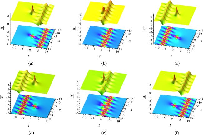
Figure 1. The interaction solutions between first-order rogue wave and one-breather wave to equation ( |
For calculation simplicity, by choosing φ1 = ϵ, ${\phi }_{2}=-\tfrac{\pi }{6}$, ${\phi }_{3}=\tfrac{\pi }{3}$, φ4 = ϵ + π, ${\phi }_{5}=\tfrac{5\pi }{6}$, ${\phi }_{6}=\tfrac{4\pi }{3}$, c1 = − 1, c4 = − 1, $\sigma =\tfrac{1}{8}$ and ϵ → 0 for equation (2 ) with N = 3, we obtain the interaction solutions among the first-order rogue wave and two-breather waves, which are not shown here because of the complex expression. In figure 2, we demonstrate the effect of the parameters c2, c3, c5 and c6 on the collision among the first-order rogue wave and two-breather waves. From figure 2(a), the first-order rogue wave is in the middle of the two-breather waves. With the increase of the parameters c2, c3, c5 and c6 from −10 to $-\tfrac{1}{60}$, two Akhmediev breather waves move in opposite directions. Collisions occur among the first-order rogue wave and two-breather waves. After the collisions, the shape of them remains unchanged. When the parameters c2, c3, c5 and c6 increase from $\tfrac{1}{60}$ to 10, the direction of movement of the two-breather waves changes. They collide with the first-order rogue wave, and then gradually move away.
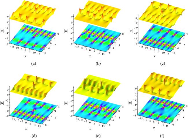
Figure 2. The interaction solutions among the first-order rogue wave and two-breather waves to equation ( |
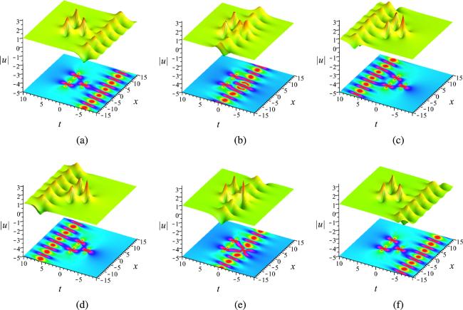
To discuss the interaction phenomena between the second-order rogue wave and one-breather wave, according to the process of constructing the second-order rogue wave solutions, the parameters are taken as follows φ1 = 2ϵ, φ2 = − ϵ, ${\phi }_{3}=-\tfrac{\pi }{3}$, φ4 = 2ϵ + π, φ5 = − ϵ + π, ${\phi }_{6}=\tfrac{2\pi }{3}$, ${c}_{1}=\tfrac{1}{3}+\tfrac{1}{3}{\varepsilon }^{2}$, ${c}_{2}=-\tfrac{1}{3}{\varepsilon }^{3}-10$, ${c}_{4}=\tfrac{1}{3}+\tfrac{1}{3}{\varepsilon }^{2}$, ${c}_{5}=-\tfrac{1}{3}{\varepsilon }^{3}-10$, $\sigma =\tfrac{1}{8}$ and ϵ → 0 for equation (2 ) with N = 3. Figure 3 clearly indicates that the position of the second-order rogue wave and the breather wave is dependent on the parameters c3 and c6. The Akhmediev breather wave moves toward the positive axis of time when parameters c3 and c6 are negative. The direction of the Akhmediev breather wave changes when the parameter becomes positive. Two collisions occur in this process. The Akhmediev breather wave can pass through the second-order rogue wave. The shape of them is not changed by the collisions.
Figure 3. The interaction solutions between the second-order rogue wave and one-breather wave to equation ( |
Compared with the interaction solutions in [50], collisions occur among the rogue wave and breather wave by choosing and controlling the parameters related to the phase in this paper. Different from the two crossed breather waves in figure 8 of [50], the two-breather waves in figure 2 are parallel. For the interaction solutions between the second-order rogue wave and one-breather wave, figure 3 shows richer interaction phenomena than that in [51] by controlling the parameters c3 and c6. The direction of movement of the breather wave is determined by the sign of the parameters c3 and c6. The breather wave can pass through the second-order rogue wave. The shape of them remains unchanged after the collisions.
4. Conclusions
Based on the long wave limit method, the second-order and third-order rogue wave solutions to the focusing NLS equation have been obtained by introducing some arbitrary parameters. The expression of the rogue wave solutions is more general than that in [26]. The interaction solutions between the first-order rogue wave and one-breather wave have been derived by taking a long wave limit on the N-breather solutions with N = 2. By applying the same method to the N-breather solutions with N = 3, two types of interaction solutions among the first-order rogue wave and two-breather waves, the second-order rogue wave and one-breather wave have been constructed, respectively. The influence of the parameters related to the phase on the interaction phenomena has been analyzed. Compared with the interaction solutions obtained by the generalized Darboux transformation [50], collisions occur among the rogue waves and breather waves. After the collisions, the shape of them remains unchanged. This paper presents abundant interaction phenomena and provides possible ways to control collisions among nonlinear waves. In the future, we aim to explore high-order rogue wave solutions and interaction solutions to other nonlinear equations.