


1. Introduction
The nonlinear Schrödinger (NLS) equation, which incorporates higher-order dispersive terms, is widely used in the theoretical analysis of various physical phenomena, including nonlinear optics, molecular systems, and fluid dynamics [1-5]. With the addition of fourth-order terms, known as the Lakshmanan-Porsezian-Daniel (LPD) equation, it describes higher-order molecular excitations with quadruple-quadruple coefficients and possesses integrability [6-8]. Lakshmanan et al investigated its application to study nonlinear spin excitations involving bilinear and biquadratic interactions [7]. In recent years, Ankiewicz et al introduced a further extension of the NLS equation by incorporating third-order (odd) and fourth-order (even) dispersion terms The NLS equation with higher-order terms becomes increasingly significant when modeling the propagation of ultra-short optical pulses along optical fibers [9, 10]. The integrability of the extended NLS equation, with certain parameter values, was confirmed in [11], where Lax operators were introduced. We now write this equation as it appears in the aforementioned references with some modification as
$\begin{eqnarray}\begin{array}{c}{\rm{i}}{u}_{t}+{\alpha }_{2}\left({u}_{{xx}}+2u|u{|}^{2}\right)+{\rm{i}}{\alpha }_{1}\left({u}_{{xxx}}+6{u}_{x}|u{|}^{2}\right)\\ +\gamma ({u}_{{xxxx}}+6\bar{u}{u}_{x}^{2}+4u|{u}_{x}{|}^{2}\\ +8|u{|}^{2}{u}_{{xx}}+2{u}^{2}{\bar{u}}_{{xx}}+6u|u{|}^{4})=0,\end{array}\end{eqnarray}$
where u = u(x, t) is a complex-valued scalar function, and $\bar{u}$ represents its complex conjugate. This equation includes several particular cases, such as the standard NLS equation with α1 = γ = 0 [14], the Hirota equation with γ = 0 [15], and the LPD equation with α1 = 0 [7].In this study, we explore the non-commutative extension of the higher-order NLS (HNLS) equation (1.1 ). Non-commutative integrable systems have attracted considerable attention due to their relevance in quantum field theories, D-brane dynamics, and string theories [16-18]. The non-commutative version of the NLS model is significant for exploring the behavior of quantum systems and wave propagation in scenarios where non-commutativity is a fundamental aspect [19]. Non-commutativity often arises from phase-space quantization, introducing non-commutativity among independent variables through a star product [20, 21]. Our approach to inducing non-commutativity in a given nonlinear evolution equation parallels the methods employed by Lechtenfeld et al [22], Gilson and Nimmo [23], and Gilson and Macfarlane [24] for the non-commutative generalization of the sine-Gordon, Kadomtsev-Petviashvili, and Davey-Stewartson equations, respectively.
We adopt a systematic method to extend the chosen equation to its non-commutative form, without explicitly specifying the nature of non-commutativity. We consider real or complex-valued functions, such as g1 = g1(x, t) and g2 = g2(x, t), as non-commutative and take advantage of the same Lax pair as in the commutative scenario to describe the equation of nonlinear evolution.
In this paper, we investigate a non-commutative version of the HNLS equation (nc-HNLS). We define the Lax pair for the nc-HNLS equation within this context. To find solutions to the nc-HNLS equation, we construct the Darboux matrix and the binary Darboux matrix. We present explicit quasi-Gramian solutions for the non-commutative fields of the nc-HNLS equation which, after reducing the non-commutativity limit, can be reduced to a ratio of Gramian solutions.
2. Modulation instability
The propagation of a continuous or quasi-continuous wave triggers modulational instability (MI), a phenomenon arising from the interplay of dispersion and nonlinear interactions [25-27]. MI serves as a valuable tool for numerically investigating the mechanisms behind solution generation within the framework of nonlinear equations. By splitting the MI and modulational stability zones, we can determine the circumstances to excite plane waves, solitons, breather and rogue waves. This approach facilitates a comprehensive understanding of the dynamics governing wave phenomena in nonlinear dispersive media. To analyze the modulation instability, we give a plane-wave solution of the equation (1.1 ) as 2.1 ) holds significant importance in the realm of optics, particularly within the context of the NLS equation. This solution represents a wave with constant amplitude that undergoes a nonlinear evolution over time. The dynamics are determined by parameters such as the amplitude c, the constant γ, and α2. This solution's application extends to the study of the stability of plane waves and comprehension of the generation of periodic patterns through MI. It serves as a prime example of how the NLS equation can lead to complex behavior in optical systems, thereby making it a crucial area of research in this field.
$\begin{eqnarray}u(x,t)=c{{\rm{e}}}^{{\rm{i}}(6{c}^{4}\gamma +2{\alpha }_{2}{c}^{2})t}.\end{eqnarray}$
The solution provided by equation (An approach to assess the stability of the plane-wave solution involves introducing perturbations to the solution and examining the linearized evolution of these perturbations. To simplify the analysis, the common phase can be factored out of the equation. This leads to a first-order ordinary differential equation (ODE) that couples the complex field with its complex conjugate as a result of the perturbation. Substituting the perturbed function v(x, t) into equation (2.1 ), we obtain 2.2 ) into (1.1 ) and after linearization, we have
$\begin{eqnarray}u(x,t)=(c+v(x,{\unicode{x000A0}}t)){{\rm{e}}}^{{\rm{i}}(6{c}^{4}\gamma +2{\alpha }_{2}{c}^{2})t}.\end{eqnarray}$
Substituting ( $\begin{eqnarray}\begin{array}{c}{\rm{i}}{v}_{t}+{\alpha }_{2}{v}_{{xx}}+{\rm{i}}{\alpha }_{1}({v}_{{xxx}}+6{c}^{2}{v}_{x})\\ \,+\gamma {v}_{{xxxx}}+2\gamma {c}^{2}(4{v}_{{xx}}+{\bar{v}}_{{xx}})+{c}^{2}(12\gamma {c}^{2}+2{\alpha }_{2})(v+\bar{v})=0.\end{array}\end{eqnarray}$
To analyze the stability of the plane-wave solution, the Fourier transform of the equation is taken. This results in a first-order ODE that governs the real and imaginary parts of evolution. The stability of the solution can then be determined by looking at the eigenvalues of this ODE. In particular, the eigenvalues represent the exponent in the time evolution of the solution. Thus, the Fourier transform of the evolution equation (2.3 ) is
$\begin{eqnarray}\begin{array}{c}{\rm{i}}{\hat{v}}_{t}-\displaystyle \frac{{\alpha }_{2}}{2}{k}^{2}\hat{v}-{\alpha }_{1}k(-{k}^{2}+6{c}^{2})\hat{v}\\ \,+\gamma {k}^{4}\hat{v}-2\gamma {c}^{2}{k}^{2}(4\hat{v}+\bar{\hat{v}})+{c}^{2}(12\gamma {c}^{2}+2{\alpha }_{2})(\hat{v}+\bar{\hat{v}})=0.\end{array}\end{eqnarray}$
The linear evolution equation for $\hat{v}$ can be evaluated by separating it into its real and imaginary components. Thus, for $\hat{v}={v}_{1}+{\rm{i}}{v}_{2}$, we have a system of differential equations 2.6 ) is shown in figure 1.
$\begin{eqnarray}\begin{array}{l}{y}_{t}\,=\left[\begin{array}{cc}0 & \beta -6\gamma \,{c}^{2}{k}^{2}\\ -\beta -10\gamma \,{c}^{2}{k}^{2}+2{c}^{2}\left(12{c}^{2}\gamma +2{\alpha }_{2}\right) & 0\end{array}\right]y,\end{array}\end{eqnarray}$
where $\beta =\tfrac{\alpha 2\,k}{2}+{\alpha }_{1}k\left(6{c}^{2}-{k}^{2}\right)-\gamma \,{k}^{4}$, and $y={[\begin{array}{cc}{v}_{1} & {v}_{2}\end{array}]}^{T}$. One can evaluate the stability of a system by analyzing exponential solutions in the form of y = νeωt, which leads to an eigenvalue problem where the eigenvalues are then given by $\begin{eqnarray}\begin{array}{l}\omega (k)=\displaystyle \frac{| k| }{2}\sqrt{\left({\alpha }_{2}\left(-8{c}^{2}+{k}^{2}\right)-2{\alpha }_{1}k\left(-6{c}^{2}+{k}^{2}\right)-2\gamma \left(24{c}^{4}-10{c}^{2}{k}^{2}+{k}^{4}\right)\right){\beta }_{1}},\\ k{\beta }_{1}=2(\beta -6\gamma {k}^{2}{c}^{2}).\end{array}\end{eqnarray}$
The plot of equation (
Figure 1. The modulation instability gain spectrum is distributed across the amplitude of the plane-wave background and the frequency of perturbation, as derived from the plane-wave seed solution ( |
The stability of the solution becomes evident when examining a graphical representation of the real parts of eigenvalues plotted against different frequencies. If the real part is positive, the solution will exhibit growth; conversely, negative values indicate decay. The overall stability is established by observing whether the real eigenvalue remains positive or negative across various frequency ranges. This phenomenon is referred to as MI.
3. Non-commutative HNLS equation
The spectral problem associated with the nc-HNLS equation is given by 3.5 ) is a non-commutative generalization of the HNLS equation, as given in equation (1.1 ). This equation exhibits several interesting properties. For instance, when both α2 and γ are zero, it reduces to non-commutative generalization of the complex modified Korteweg-de Vries (KdV) equation and to the standard modified KdV equation for real-valued u. Moreover, setting γ to zero results in the non-commutative generalization of the Hirota equation, while setting α1 and α2 to zero simultaneously yields the well-known LPD equation. Finally, when α1 and γ are set to zero, the equation reduces to non-commutative generalization of the NLS equation. After relaxing the non-commutativity condition, equation (3.5 ) corresponds to the commutative counterpart. The spectral problem linked with equation (1.1 ) remains the same as that of equations (3.1 ) and (3.2 ), with the exception that u and $\bar{u}$ are now perceived as commutative functions.
$\begin{eqnarray}{\rm{\Gamma }}={\partial }_{x}-\lambda { \mathcal J }-{ \mathcal U },\end{eqnarray}$
$\begin{eqnarray}{\rm{\Delta }}={\partial }_{t}-{ \mathcal B }-{{ \mathcal V }}_{p},\end{eqnarray}$
where $\begin{eqnarray}{ \mathcal J }=\left[\begin{array}{cc}-{\rm{i}} & 0\\ 0 & {\rm{i}}\end{array}\right],\quad { \mathcal U }=\left[\begin{array}{cc}0 & u\\ -{u}^{\dagger } & 0\end{array}\right],\quad {{ \mathcal V }}_{p}=\gamma \left[\begin{array}{cc}{{ \mathcal V }}_{1} & {{ \mathcal V }}_{2}\\ {{ \mathcal V }}_{3} & {{ \mathcal V }}_{4}\end{array}\right],\end{eqnarray}$
$\begin{eqnarray}\begin{array}{l}{ \mathcal B }\,=\left(\begin{array}{lc}{\rho }_{1}+{\rho }_{2}{{uu}}^{\dagger }-{\alpha }_{1}\left(\left(\displaystyle \frac{\partial }{\partial x}u\right){u}^{\dagger }-u\left(\displaystyle \frac{\partial }{\partial x}{u}^{\dagger }\right)\right) & {{ \mathcal A }}_{2}\\ {{ \mathcal A }}_{1} & -{\rho }_{1}-{\rho }_{2}{u}^{\dagger }u-{\alpha }_{1}\left(-{u}^{\dagger }\left(\displaystyle \frac{\partial }{\partial x}u\right)+\left(\displaystyle \frac{\partial }{\partial x}{u}^{\dagger }\right)u\right)\end{array}\right),\end{array}\end{eqnarray}$
$\begin{eqnarray*}\begin{array}{l}{{ \mathcal A }}_{1}=-4{\lambda }^{2}{\alpha }_{1}{u}^{\dagger }+2\lambda \left(-{\alpha }_{2}{u}^{\dagger }+{\rm{i}}{\alpha }_{1}\left(\displaystyle \frac{\partial }{\partial x}{u}^{\dagger }\right)\right)+{\rm{i}}{\alpha }_{2}\left(\displaystyle \frac{\partial }{\partial x}{u}^{\dagger }\right)\\ -{\alpha }_{1}\left(-2{u}^{\dagger }{{uu}}^{\dagger }-\displaystyle \frac{{\partial }^{2}}{\partial {x}^{2}}{u}^{\dagger }\right),\\ {{ \mathcal A }}_{2}=4{\lambda }^{2}{\alpha }_{1}u+2\lambda \left({\alpha }_{2}u+{\rm{i}}{\alpha }_{1}\left(\displaystyle \frac{\partial }{\partial x}u\right)\right)\\ +{\rm{i}}{\alpha }_{2}\left(\displaystyle \frac{\partial }{\partial x}u\right)-{\alpha }_{1}\left(2{{uu}}^{\dagger }u+\displaystyle \frac{{\partial }^{2}}{\partial {x}^{2}}u\right),\\ {{ \mathcal V }}_{1}={\rm{i}}\left(\left(\displaystyle \frac{{\partial }^{2}}{\partial {x}^{2}}u\right){u}^{\dagger }+u\left(\displaystyle \frac{{\partial }^{2}}{\partial {x}^{2}}{u}^{\dagger }\right)-\left(\displaystyle \frac{\partial }{\partial x}u\right)\left(\displaystyle \frac{\partial }{\partial x}{u}^{\dagger }\right)\right)\\ -2\lambda \left(u\left(\displaystyle \frac{\partial }{\partial x}{u}^{\dagger }\right)-\left(\displaystyle \frac{\partial }{\partial x}u\right){u}^{\dagger }\right)+{\rho }_{3},\\ {{ \mathcal V }}_{2}=-4\,{\rm{i}}{\lambda }^{2}\left(\displaystyle \frac{\partial }{\partial x}u\right)+3\,{\rm{i}}\left({{uu}}^{\dagger }\left(\displaystyle \frac{\partial }{\partial x}u\right)\right.\\ \left.+\left(\displaystyle \frac{\partial }{\partial x}u\right){u}^{\dagger }u\right)+{\rm{i}}\left(\displaystyle \frac{{\partial }^{3}}{\partial {x}^{3}}u\right)+2\lambda \left(\displaystyle \frac{{\partial }^{2}}{\partial {x}^{2}}u\right)+{\rho }_{5},\\ {{ \mathcal V }}_{3}=-4\,{\rm{i}}{\lambda }^{2}\left(\displaystyle \frac{\partial }{\partial x}{u}^{\dagger }\right)+3\,{\rm{i}}\left({u}^{\dagger }u\left(\displaystyle \frac{\partial }{\partial x}{u}^{\dagger }\right)\right.\end{array}\end{eqnarray*}$
$\begin{eqnarray*}\begin{array}{l}\left.+\left(\displaystyle \frac{\partial }{\partial x}{u}^{\dagger }\right){{uu}}^{\dagger }\right)+{\rm{i}}\left(\displaystyle \frac{{\partial }^{3}}{\partial {x}^{3}}{u}^{\dagger }\right)-2\lambda \left(\displaystyle \frac{{\partial }^{2}}{\partial {x}^{2}}{u}^{\dagger }\right)+{\rho }_{6},\\ {{ \mathcal V }}_{4}=-{\rm{i}}\left(\left(\displaystyle \frac{{\partial }^{2}}{\partial {x}^{2}}{u}^{\dagger }\right)u+{u}^{\dagger }\left(\displaystyle \frac{{\partial }^{2}}{\partial {x}^{2}}u\right)\right.\\ \left.-\left(\displaystyle \frac{\partial }{\partial x}{u}^{\dagger }\right)\left(\displaystyle \frac{\partial }{\partial x}u\right)\right)\\ +2\lambda \left(-{u}^{\dagger }\left(\displaystyle \frac{\partial }{\partial x}u\right)+\left(\displaystyle \frac{\partial }{\partial x}{u}^{\dagger }\right)u\right)+{\rho }_{4},\end{array}\end{eqnarray*}$
where ρ1 = − 4 iα1λ3 − 2 iλ2α2, ρ2 = i(2λα1 + α2), ρ3 = 3 iuu†uu† − 4 iλ2uu† + 8 iλ4, ρ4 = − 3 iu†uu†u + 4 iλ2u†u − 8 iλ4, ρ5 = − 8λ3u + 4λuu†u, ρ6 = 8λ3u† − 4λu†uu†. The equation of motion for the system can be derived by setting the commutator of Γ and Δ equal to zero and equating the coefficients at λ $\begin{eqnarray}\begin{array}{l}{\rm{i}}{u}_{t}+{\rm{i}}\left({u}_{{xxx}}+3({u}_{x}{u}^{\dagger }u+{{uu}}^{\dagger }{u}_{x})\right){\alpha }_{1}\\ \,+\left(2{{uu}}^{\dagger }u+{u}_{{xx}}\right){\alpha }_{2}\\ +({u}_{{xxxx}}+2({u}_{x}{u}_{x}^{\dagger }u+{{uu}}_{x}^{\dagger }{u}_{x}+{{uu}}_{{xx}}^{\dagger }u)\\ \,+4({u}_{{xx}}{u}^{\dagger }u+{{uu}}^{\dagger }{u}_{{xx}})\\ +6({u}_{x}{u}^{\dagger }{u}_{x}+{{uu}}^{\dagger }{{uu}}^{\dagger }u))\gamma =0,\end{array}\end{eqnarray}$
where u = u(x, t) is an non-commutative object, † denotes the adjoint (Hermitian conjugate), α1, α2, and γ are real parameters, and λ is a spectral parameter (real or complex). The equation presented in (3.1. Quasideterminants
In non-commutative algebra, quasideterminants serve as a replacement for ordinary determinants of matrices. They hold a similar significance in non-commutative algebra as ordinary determinants do in commutative algebra and have found vast applications in the domain of non-commutative integrable systems [23, 28, 29].
The quasideterminant ∣M∣ij for i, j = 1,..., n of an n × n matrix over a non-commutative ring R, expanded about the matrix mij, is defined as
$\begin{eqnarray}{\left|M\right|}_{{ij}}=\left|\begin{array}{cc}{M}^{{ij}} & {c}_{j}^{i}\\ {r}_{i}^{j} & \boxed{{m}_{{ij}}}\end{array}\right|={m}_{{ij}}-{r}_{i}^{j}{\left({M}^{{ij}}\right)}^{-1}{c}_{j}^{i},\end{eqnarray}$
where mij is referred to as the expansion point and represents the ijth entry of M, rji denotes the ith row of M without the jth entry, cij represents the jth column of M without the ith row, and Mij is the submatrix of M obtained by removing the ith row and the jth column from M.Quasideterminants are not merely a generalization of usual commutative determinants but are also related to inverse matrices. The inverse of a matrix $M=\left(\begin{array}{cc}{m}_{11} & {m}_{12}\\ {m}_{21} & {m}_{22}\end{array}\right)$ is defined as
$\begin{eqnarray}\begin{array}{l}{M}^{-1}=\left(| M{| }_{{ji}}^{-1}\right)=\left(\begin{array}{cc}{\left|\begin{array}{cc}\boxed{{m}_{11}} & {m}_{12}\\ {m}_{21} & {m}_{22}\end{array}\right|}^{-1} & {\left|\begin{array}{cc}{m}_{11} & \boxed{{m}_{12}}\\ {m}_{21} & {m}_{22}\end{array}\right|}^{-1}\\ {\left|\begin{array}{cc}{m}_{11} & {m}_{12}\\ \boxed{{m}_{21}} & {m}_{22}\end{array}\right|}^{-1} & {\left|\begin{array}{cc}{m}_{11} & {m}_{12}\\ {m}_{21} & \boxed{{m}_{22}}\end{array}\right|}^{-1}\end{array}\right).\end{array}\end{eqnarray}$
4. Darboux transformation
The application of quasideterminants when solving non-commutative (or matrix) nonlinear equations has proven to be an effective tool, particularly in generating multisoliton solutions. The Darboux transformation (DT), as demonstrated in many works, such as [24, 29-33], provides a systematic and effective approach for constructing these diverse solutions. This transformative methodology contributes significantly to understanding complex phenomena in nonlinear systems, providing insights into the formation and dynamics of bright solitons, multi-valley dark solitons, and high-order rogue waves. In this section, a DT is introduced for the system of the nc-HNLS equation (3.5 ) through the definition of the Darboux matrix 3.3 ) and (3.4 ), respectively, are utilized as entries in the Lax operators. Now, consider a function φ = φ(x, t) that is an eigenfunction of the Lax operators Γ and Δ such that Γ(φ) = 0 and Δ(φ) = 0. We can define a new function $\tilde{\varphi }$ using the Darboux matrix $D({ \mathcal Y })$:
$\begin{eqnarray}\begin{array}{l}D({ \mathcal Y })=\lambda I-{ \mathcal Y }{\rm{\Lambda }}{{ \mathcal Y }}^{-1},\end{array}\end{eqnarray}$
and the Lax operators Γ and Δ $\begin{eqnarray}{\rm{\Gamma }}={\partial }_{x}-\lambda { \mathcal J }-{ \mathcal U },\quad {\rm{\Delta }}={\partial }_{t}-{ \mathcal B }-{{ \mathcal V }}_{p}.\end{eqnarray}$
The spectral parameter λ, which can be real or complex, is incorporated together with the constant q × q matrix Λ, and the non-commutative objects ${ \mathcal U },\ {{ \mathcal V }}_{p}$, and ${ \mathcal B }$ from equations ( $\begin{eqnarray}\begin{array}{l}\tilde{\varphi }:= {D}_{{ \mathcal Y }}(\varphi ),\\ =\lambda \varphi -{ \mathcal Y }{\rm{\Lambda }}{{ \mathcal Y }}^{-1}\phi =\left|\begin{array}{cc}{ \mathcal Y } & \varphi \\ { \mathcal Y }{\rm{\Lambda }} & \boxed{\lambda \varphi }\end{array}\right|.\end{array}\end{eqnarray}$
The function $\tilde{\varphi }$ is a generic function of the new operators $\tilde{{\rm{\Gamma }}}={D}_{{ \mathcal Y }}{\rm{\Gamma }}{D}_{{ \mathcal Y }}^{-1}$ and $\tilde{{\rm{\Delta }}}={D}_{{ \mathcal Y }}{\rm{\Delta }}{D}_{{ \mathcal Y }}^{-1}$. Next,we define ${{ \mathcal Y }}_{[1]}={{ \mathcal Y }}_{1}$ and φ[1]=φ as generic eigenfunctions of Γ[1]=Γ and Δ[1]=Δ, where ${{ \mathcal Y }}_{1}$ and φ1 are 2 × 2 matrices. We then define ${\varphi }_{[2]}={D}_{{{ \mathcal Y }}_{[1]}}\left({\varphi }_{[1]}\right)$ and ${{ \mathcal Y }}_{[2]}={\varphi }_{[2]}{| }_{\varphi \to {{ \mathcal Y }}_{2}}$ to be eigenfunctions of the new operators ${{\rm{\Gamma }}}_{[2]}={D}_{{{ \mathcal Y }}_{[1]}}{{\rm{\Gamma }}}_{[1]}{D}_{{{ \mathcal Y }}_{[1]}}^{-1}$ and ${{\rm{\Delta }}}_{[2]}\,={D}_{{{ \mathcal Y }}_{[1]}}{{\rm{\Delta }}}_{[1]}{D}_{{{ \mathcal Y }}_{[1]}}^{-1}$.We define ${{ \mathcal Y }}_{i},\ i=1,...,\ n$ (where each ${{ \mathcal Y }}_{i}$ is a matrix of size 2 × 2) to be the set of particular eigenfunctions of Γ and Δ. In the non-commutative case, we consider each entry of ${{ \mathcal Y }}_{i}$ as a matrix. We define the (n + 1)th eigenfunction as ${\varphi }_{[n+1]}={D}_{{{ \mathcal Y }}_{[n]}}\left({\varphi }_{[n]}\right)$, which is a generic eigenfunction of the new operators ${{\rm{\Gamma }}}_{[n+1]}={D}_{{{ \mathcal Y }}_{[n]}}{{\rm{\Gamma }}}_{[n]}{D}_{{{ \mathcal Y }}_{[n]}}^{-1}$, and ${{\rm{\Delta }}}_{[n+1]}\,={D}_{{{ \mathcal Y }}_{[n]}}{{\rm{\Delta }}}_{[n]}{D}_{{{ \mathcal Y }}_{[n]}}^{-1}$. Here, ${{ \mathcal Y }}_{[n]}$ is a DT from Γ[n] to Γ[n+1] and Δ[n] to Δ[n+1]. Thus, the nth-order DT is given by ${\varphi }_{[n+1]}={D}_{{{ \mathcal Y }}_{[n]}}\left({\varphi }_{[n]}\right)=\lambda {\varphi }_{[n]}-{{ \mathcal Y }}_{[n]}{{\rm{\Lambda }}}_{n}{{ \mathcal Y }}_{[n]}^{-1}{\varphi }_{[n]}$, where ${{ \mathcal Y }}_{[j]}={\varphi }_{[j]}{| }_{\varphi \to {{ \mathcal Y }}_{j}}$. Let us define a matrix ${\rm{\Xi }}=({{ \mathcal Y }}_{1},...,\ {{ \mathcal Y }}_{n})$ comprising the eigenfunctions ${{ \mathcal Y }}_{i},\ i=1,...,\ n$, and set φ[1] = φ. Then, we can represent the nth iteration of the DT in quasideterminant form given by
$\begin{eqnarray}\begin{array}{c}{\varphi }_{\left[n+1\right]}=\left|\begin{array}{cc}{\rm{\Xi }} & \varphi \\ \vdots & \vdots \\ {{\rm{\Xi }}}^{\left(n-1\right)} & {\varphi }^{\left(n-1\right)}\\ {{\rm{\Xi }}}^{\left(n\right)} & \boxed{\displaystyle {\varphi }^{\left(n\right)}}\end{array}\right|.\end{array}\end{eqnarray}$
Here, φ(n) = λnφ and Ξ(n) = ΞΛn, where each Λi, i = 1,..., n, is a constant matrix. Hence, we expressed a quasideterminant formula for φ[n+1] in terms of the known eigenfunctions ${{ \mathcal Y }}_{i},\ i=1,...,\ n$ and the eigenfunction φ of the “seed” Lax pair Γ = Γ1, Δ = Δ1.5. Quasi-Wronskian solutions
In the upcoming analysis, we will examine how the DT, ${D}_{{ \mathcal Y }}=\lambda I-{ \mathcal Y }{\rm{\Lambda }}{{ \mathcal Y }}^{-1}$, affects the Lax operator Γ = Γ1, where ${ \mathcal Y }$ is an eigenfunction of Γ (since ${\rm{\Gamma }}({ \mathcal Y })=0$ by definition) and Λ is an eigenvalue matrix. It is important to note that the same results apply to the operator Δ = Δ1. As a result of this transformation, the operator Γ is converted to a new operator $\tilde{{\rm{\Gamma }}}={{\rm{\Gamma }}}_{[2]}$, which can be expressed as $\tilde{{\rm{\Gamma }}}={D}_{{ \mathcal Y }}{\rm{\Gamma }}{D}_{{ \mathcal Y }}^{-1}$. By substituting equations (3.1 ) and (4.1 ) into the latter equation and equating the coefficients at λj, we obtain two equations, 5.2 ), we express equation (3.1 ) using a particular eigenfunction ${ \mathcal Y }$ as ${{ \mathcal Y }}_{x}={ \mathcal J }{ \mathcal Y }{\rm{\Lambda }}+{ \mathcal U }{ \mathcal Y }$. By utilizing this equation, we can easily check that the condition expressed in equation (5.2 ) is satisfied. To simplify the notation, a matrix ${ \mathcal F }$ is introduced such that ${ \mathcal U }=[{ \mathcal F },\ { \mathcal J }]$. This equation is satisfied if ${ \mathcal F }=\tfrac{1}{2{\rm{i}}}\left(\begin{array}{cc}0 & u\\ {u}^{\dagger } & 0\end{array}\right)$. Then, equation (5.1 ) with ${ \mathcal U }=[{ \mathcal F },\ { \mathcal J }]$ can be used to obtain ${{ \mathcal F }}_{[2]}={ \mathcal F }-{{ \mathcal Y }}^{(1)}{{ \mathcal Y }}^{-1}$, where ${{ \mathcal Y }}^{(1)}$ is defined as ${ \mathcal Y }{\rm{\Lambda }}$. After n repeated applications of the DT ${D}_{{ \mathcal Y }}$, we have
$\begin{eqnarray}{{ \mathcal U }}_{[2]}-{ \mathcal U }-[{ \mathcal J },\ { \mathcal Y }{\rm{\Lambda }}{{ \mathcal Y }}^{-1}]=0,\end{eqnarray}$
and $\begin{eqnarray}-{\partial }_{x}({ \mathcal Y }{\rm{\Lambda }}{{ \mathcal Y }}^{-1})+[{ \mathcal U },\ { \mathcal Y }{\rm{\Lambda }}{{ \mathcal Y }}^{-1}]+[{ \mathcal J },\ { \mathcal Y }{\rm{\Lambda }}{{ \mathcal Y }}^{-1}]{ \mathcal Y }{\rm{\Lambda }}{{ \mathcal Y }}^{-1}=0.\end{eqnarray}$
To confirm the validity of equation ( $\begin{eqnarray}\begin{array}{l}{{ \mathcal F }}_{[n+1]}={{ \mathcal F }}_{[n]}-{{ \mathcal Y }}_{[n]}^{(1)}{{ \mathcal Y }}_{[n]}^{-1}\\ ={ \mathcal F }-\displaystyle \sum _{k=1}^{n}{{ \mathcal Y }}_{[k]}^{(1)}{{ \mathcal Y }}_{[k]}^{-1},\end{array}\end{eqnarray}$
where ${{ \mathcal F }}_{[1]}={ \mathcal F },\ {{ \mathcal Y }}_{[1]}={{ \mathcal Y }}_{1}={ \mathcal Y }$, and Λ1 = Λ.Because our nc-HNLS equation (3.5 ) is expressed in terms of u and u†, it is more appropriate to express the quasi-Wronskian solution in terms of these objects. For this, we express each ${{ \mathcal Y }}_{i},\ i=1,...,\ n$ as a 2 × 2 matrix as ${{ \mathcal Y }}_{i}=\left(\begin{array}{cc}{\varphi }_{2i-1} & {\varphi }_{2i}\\ {\chi }_{2i-1} & {\chi }_{2i}\end{array}\right)$. For φ = φ(x, t) and χ = χ(x, t), we can express ${{ \mathcal F }}_{[n+1]}$ as
$\begin{eqnarray}{{ \mathcal F }}_{[n+1]}={ \mathcal F }+\left(\begin{array}{cc}\left|\begin{array}{cc}\widehat{{\rm{\Xi }}} & {f}_{2n-1}\\ {\varphi }^{(n)} & \boxed{0}\end{array}\right| & \left|\begin{array}{cc}\widehat{{\rm{\Xi }}} & {f}_{2n}\\ {\varphi }^{(n)} & \boxed{0}\end{array}\right|\\ \left|\begin{array}{cc}\widehat{{\rm{\Xi }}} & {f}_{2n-1}\\ {\chi }^{(n)} & \boxed{0}\end{array}\right| & \left|\begin{array}{cc}\widehat{{\rm{\Xi }}} & {f}_{2n}\\ {\chi }^{(n)} & \boxed{0}\end{array}\right|\end{array}\right),\end{eqnarray}$
where $\widehat{{\rm{\Xi }}}={({{ \mathcal Y }}_{j}^{(i-1)})}_{i,\ j\,=\,1,...,\ n}$ is the 2n × 2n matrix of ${{ \mathcal Y }}_{1},...,\ {{ \mathcal Y }}_{n}$, and f2n−1 and f2n are the column vectors 2n × 1 with a 1 in the (2n − 1)th and (2n)th rows, respectively, and zeros elsewhere, while ${\varphi }^{(n)}=\left({\varphi }_{1}^{(n)},...,\ {\varphi }_{2n}^{(n)}\right),\ {\chi }^{(n)}=\left({\chi }_{1}^{(n)},...,\ {\chi }_{2n}^{(n)}\right)$ denote the 1 × 2n row vectors. We can express the quasi-Wronskian solutions for u and u† by utilizing ${ \mathcal F }=\tfrac{1}{2{\rm{i}}}\left(\begin{array}{cc}0 & u\\ {u}^{\dagger } & 0\end{array}\right)$, so that $\begin{eqnarray}\begin{array}{l}{u}_{[n+1]}=u+2{\rm{i}}\left|\begin{array}{cc}\widehat{{\rm{\Xi }}} & {f}_{2n}\\ {\varphi }^{(n)} & \boxed{0}\end{array}\right|,\\ {u}_{[n+1]}^{\dagger }={u}^{\dagger }+2{\rm{i}}\left|\begin{array}{cc}\widehat{{\rm{\Xi }}} & {f}_{2n-1}\\ {\chi }^{(n)} & \boxed{0}\end{array}\right|.\end{array}\end{eqnarray}$
We proceed in the next section to construct the binary DT for the nc-HNLS equation, using a strategy similar to that employed in [12].6. Binary Darboux transformation
We introduce ${{ \mathcal Y }}_{1},...,\ {{ \mathcal Y }}_{n}$ as eigenfunctions of the Lax operators Γ and Δ, and ${{ \mathcal Z }}_{1},...,\ {{ \mathcal Z }}_{n}$ as eigenfunctions of the adjoint Lax operators Γ† and Δ†. Assuming φ[1] = φ to be a generic eigenfunction of the Lax operators Γ and Δ, and ψ[1] = ψ to be a generic eigenfunction of the adjoint Lax operators Γ† and Δ†, we define the binary DT and its adjoint as
$\begin{eqnarray}{D}_{{{ \mathcal Y }}_{[1]},\ {{ \mathcal Z }}_{[1]}}=I-{{ \mathcal Y }}_{[1]}{\rm{\Upsilon }}{\left({{ \mathcal Y }}_{[1]},\ {{ \mathcal Z }}_{[1]}\right)}^{-1}{{\rm{\Omega }}}^{-\dagger }{{ \mathcal Z }}_{[1]}^{\dagger },\end{eqnarray}$
$\begin{eqnarray}{D}_{{{ \mathcal Y }}_{[1]},\ {{ \mathcal Z }}_{[1]}}^{\dagger }=I-{{ \mathcal Z }}_{[1]}{\rm{\Upsilon }}{\left({{ \mathcal Y }}_{[1]},\ {{ \mathcal Z }}_{[1]}\right)}^{-\dagger }{{\rm{\Lambda }}}^{-\dagger }{{ \mathcal Y }}_{[1]}^{\dagger }.\end{eqnarray}$
Within the context of the binary DT, we use ${{ \mathcal Y }}_{[1]}={{ \mathcal Y }}_{1}$ as the initial eigenfunction that characterizes the transformation from the Lax operators Γ and Δ to the new operators $\tilde{{\rm{\Gamma }}}$ and $\tilde{{\rm{\Delta }}}$. Similarly, we define ${{ \mathcal Z }}_{[1]}={{ \mathcal Z }}_{1}$ to represent the adjoint transformation, where the potential ϒ $\begin{eqnarray}{{\rm{\Omega }}}^{\dagger }{\rm{\Upsilon }}({{ \mathcal Y }}_{[1]},\ {{ \mathcal Z }}_{[1]})+{\rm{\Upsilon }}({{ \mathcal Y }}_{[1]},\ {{ \mathcal Z }}_{[1]}){\rm{\Lambda }}={{ \mathcal Z }}_{[1]}^{\dagger }{{ \mathcal Y }}_{[1]},\end{eqnarray}$
$\begin{eqnarray}\left(\lambda I+{{\rm{\Omega }}}^{\dagger }\right){\rm{\Upsilon }}({\varphi }_{[1]},\ {{ \mathcal Z }}_{[1]})={{ \mathcal Z }}_{[1]}^{\dagger }{\varphi }_{[1]},\end{eqnarray}$
$\begin{eqnarray}{\rm{\Upsilon }}({{ \mathcal Y }}_{[1]},\ {\psi }_{[1]})\left({\mu }^{\dagger }I+{\rm{\Lambda }}\right)={\psi }_{[1]}^{\dagger }{{ \mathcal Y }}_{[1]}.\end{eqnarray}$
The transformed operators $\widetilde{{\rm{\Gamma }}}={{\rm{\Gamma }}}_{[2]}$ and $\widetilde{{\rm{\Delta }}}={{\rm{\Delta }}}_{[2]}$ are defined as $\begin{eqnarray}{{\rm{\Gamma }}}_{[2]}={D}_{{{ \mathcal Y }}_{[1]},\ {{ \mathcal Z }}_{[1]}}{{\rm{\Gamma }}}_{[1]}{D}_{{{ \mathcal Y }}_{[1]},\ {{ \mathcal Z }}_{[1]}}^{-1},\end{eqnarray}$
$\begin{eqnarray}{{\rm{\Delta }}}_{[2]}={D}_{{{ \mathcal Y }}_{[1]},\ {{ \mathcal Z }}_{[1]}}{{\rm{\Delta }}}_{[1]}{D}_{{{ \mathcal Y }}_{[1]},\ {{ \mathcal Z }}_{[1]}}^{-1},\end{eqnarray}$
with a generic eigenfunction $\begin{eqnarray}\begin{array}{c}{\varphi }_{\left[2\right]}:={D}_{{{ \mathcal Y }}_{\left[1\right]},{{ \mathcal Z }}_{\left[1\right]}}({\varphi }_{\left[1\right]}),\\ ={\varphi }_{\left[1\right]}-{{ \mathcal Y }}_{\left[1\right]}{\rm{\Upsilon }}{\left({{ \mathcal Y }}_{\left[1\right]},{{ \mathcal Z }}_{\left[1\right]}\right)}^{-1}\\ \times \,(I+\lambda I{{\rm{\Omega }}}^{-\dagger }){\rm{\Upsilon }}({\varphi }_{\left[1\right]},{\unicode{x000A0}}{{ \mathcal Z }}_{\left[1\right]}),\end{array}\end{eqnarray}$
and with a generic adjoint eigenfunction $\begin{eqnarray}\begin{array}{l}{\psi }_{[2]}:= {D}_{{{ \mathcal Y }}_{[1]},\ {{ \mathcal Z }}_{[1]}}^{-\dagger }({\psi }_{[1]}),\\ ={\psi }_{[1]}-{{ \mathcal Z }}_{[1]}{\rm{\Upsilon }}{\left({{ \mathcal Y }}_{[1]},\ {{ \mathcal Z }}_{[1]}\right)}^{-\dagger }\\ \times \,(I+\mu I{{\rm{\Lambda }}}^{-\dagger }){\rm{\Upsilon }}{\left({{ \mathcal Y }}_{[1]},\ {\psi }_{[1]}\right)}^{\dagger }.\end{array}\end{eqnarray}$
For the nth iteration of the binary DT, we choose the eigenfunction ${{ \mathcal Y }}_{[n]}$ that defines the transformation from Γ[n], Δ[n] to Γ[n+1], Δ[n+1]. Similarly, we choose the eigenfunction ${{ \mathcal Z }}_{[n]}$ for the adjoint transformation from ${{\rm{\Gamma }}}_{[n]}^{\dagger }$, ${{\rm{\Delta }}}_{[n]}^{\dagger }$ to ${{\rm{\Gamma }}}_{[n+1]}^{\dagger }$, ${{\rm{\Delta }}}_{[n+1]}^{\dagger }$. The Lax operators Γ[n] and Δ[n] exhibit covariance under the binary DT $\begin{eqnarray}{D}_{{{ \mathcal Y }}_{[n]},\ {{ \mathcal Z }}_{[n]}}=I-{{ \mathcal Y }}_{[n]}{\rm{\Upsilon }}{\left({{ \mathcal Y }}_{[n]},\ {{ \mathcal Z }}_{[n]}\right)}^{-1}{{\rm{\Omega }}}^{-\dagger }{{ \mathcal Z }}_{[n]}^{\dagger },\end{eqnarray}$
and adjoint binary DT $\begin{eqnarray}{D}_{{{ \mathcal Y }}_{[n]},\ {{ \mathcal Z }}_{[n]}}^{-\dagger }=I-{{ \mathcal Z }}_{[n]}{\rm{\Upsilon }}{\left({{ \mathcal Y }}_{[n]},\ {{ \mathcal Z }}_{[n]}\right)}^{-1}{{\rm{\Lambda }}}^{-\dagger }{{ \mathcal Y }}_{[n]}^{\dagger }.\end{eqnarray}$
The transformed operators $\begin{eqnarray}{{\rm{\Gamma }}}_{[n+1]}={D}_{{{ \mathcal Y }}_{[n]},\ {{ \mathcal Z }}_{[n]}}{{\rm{\Gamma }}}_{[n]}{D}_{{{ \mathcal Y }}_{[n]},\ {{ \mathcal Z }}_{[n]}}^{-1},\end{eqnarray}$
$\begin{eqnarray}{{\rm{\Delta }}}_{[n+1]}={D}_{{{ \mathcal Y }}_{[n]},\ {{ \mathcal Z }}_{[n]}}{{\rm{\Delta }}}_{[n]}{D}_{{{ \mathcal Y }}_{[n]},\ {{ \mathcal Z }}_{[n]}}^{-1},\end{eqnarray}$
have a generic eigenfunction $\begin{eqnarray}\begin{array}{l}{\varphi }_{[n+1]}\\ \,={\varphi }_{[n]}-{{ \mathcal Y }}_{[n]}{\rm{\Upsilon }}{\left({{ \mathcal Y }}_{[n]},\ {{ \mathcal Z }}_{[n]}\right)}^{-1}(I+\lambda I{{\rm{\Omega }}}^{-\dagger }){\rm{\Upsilon }}({\varphi }_{[n]},\ {{ \mathcal Z }}_{[n]}),\end{array}\end{eqnarray}$
and a generic adjoint eigenfunction $\begin{eqnarray}\begin{array}{l}{\psi }_{[n+1]}\\ \,={\psi }_{[n]}-{{ \mathcal Z }}_{[n]}{\rm{\Upsilon }}{\left({{ \mathcal Y }}_{[n]},\ {{ \mathcal Z }}_{[n]}\right)}^{-1}(I+\mu I{{\rm{\Lambda }}}^{-\dagger }){\rm{\Upsilon }}{\left({{ \mathcal Y }}_{[n]},\ {\psi }_{[n]}\right)}^{\dagger }.\end{array}\end{eqnarray}$
By introducing the matrices ${\rm{\Xi }}=({{ \mathcal Y }}_{1},...,\ {{ \mathcal Y }}_{n})$ and $Z=({{ \mathcal Z }}_{1},...,\ {{ \mathcal Z }}_{n})$, we can represent these findings within the framework of quasi-Gramians, yielding the following expressions $\begin{eqnarray}\begin{array}{l}{\varphi }_{[n+1]}=\left|\begin{array}{cc}{\rm{\Upsilon }}({\rm{\Xi }},\ Z) & (I+\lambda I{\hat{{\rm{\Omega }}}}^{-\dagger }){\rm{\Upsilon }}(\varphi ,\ Z)\\ {\rm{\Xi }} & \boxed{\varphi }\end{array}\right|,\\ {\psi }_{[n+1]}=\left|\begin{array}{cc}{\rm{\Upsilon }}{\left({\rm{\Xi }},\ Z\right)}^{\dagger } & (I+\mu I{\hat{{\rm{\Lambda }}}}^{-\dagger }){\rm{\Upsilon }}{\left({\rm{\Xi }},\ \psi \right)}^{\dagger }\\ Z & \boxed{\psi }\end{array}\right|,\end{array}\end{eqnarray}$
where $\hat{{\rm{\Omega }}}=\mathrm{diag}({\rm{\Omega }},...,\ {\rm{\Omega }}),\ \hat{{\rm{\Lambda }}}=\mathrm{diag}({\rm{\Lambda }},...,\ {\rm{\Lambda }})$, where both Ω and Λ are 22 matrices.7. Quasi-Gramian solutions
In this section, we now determine the effect of binary DT ${D}_{{ \mathcal Y },\ { \mathcal Z }}=I-\xi {\rm{\Upsilon }}{({ \mathcal Y },\ { \mathcal Z })}^{-1}{{\rm{\Omega }}}^{-\dagger }{{ \mathcal Z }}^{\dagger }$ on the Lax operator Γ, with ${{ \mathcal Y }}_{1},...,\ {{ \mathcal Y }}_{n}$ being eigenfunctions of Γ. Similarly, let ${{ \mathcal Z }}_{1},...,\ {{ \mathcal Z }}_{n}$ denote the eigenfunctions of the adjoint Lax operator Γ†. The same results apply to the operators Δ and Δ†.
As the binary DT ${D}_{{{ \mathcal Y }}_{[1]},\ {{ \mathcal Z }}_{[1]}}={D}_{{ \mathcal Y },\ { \mathcal Z }}$ combines two ordinary DTs, ${D}_{{{ \mathcal Y }}_{[1]}}={D}_{{ \mathcal Y }}$ and ${D}_{{\hat{{ \mathcal Y }}}_{[1]}}={D}_{\hat{{ \mathcal Y }}}$, it follows that the Lax operator Γ is transformed into a new Lax operator $\widehat{{\rm{\Gamma }}}$ under the binary DT, given by 7.4 ), can be expressed in the quasi-Gramian form as 7.5 ), in terms of these objects. Thus, we introduce the matrices ${{ \mathcal Y }}_{i}$ by following a similar approach to the quasi-Wronskian case. We also define Z = ΞQ†, where Q represents a constant matrix of size 2n × 2n and † denotes the Hermitian conjugate. It is noted that Ξ and Z adhere to the same dispersion relation and remain unchanged when multiplied by a constant matrix. Consequently, the quasi-Gramian solution, equation (7.5 ), can also be represented as 7.7 ) represents the quasi-Gramian solutions for the nc-HNLS equation (3.5 ). If we relax the non-commutativity condition, the equation can be simplified and expressed as a ratio of simple Gramians. In the limit of commutativity, we obtain the following expressions
$\begin{eqnarray}\hat{{\rm{\Gamma }}}={D}_{\hat{{ \mathcal Y }}}{\rm{\Gamma }}{D}_{\hat{{ \mathcal Y }}}^{-1}.\end{eqnarray}$
We have $\begin{eqnarray}\widehat{{ \mathcal U }}={ \mathcal U }+\left[{ \mathcal J },\ { \mathcal Y }{\rm{\Upsilon }}{\left({ \mathcal Y },\ { \mathcal Z }\right)}^{-1}{{ \mathcal Z }}^{\dagger }\right].\end{eqnarray}$
Since ${ \mathcal U }=[{ \mathcal F },\ { \mathcal J }]$, so that $\begin{eqnarray}\widehat{{ \mathcal F }}={ \mathcal F }-{ \mathcal Y }{\rm{\Upsilon }}{\left({ \mathcal Y },\ { \mathcal Z }\right)}^{-1}{{ \mathcal Z }}^{\dagger }.\end{eqnarray}$
After n iterations of applying the binary DT ${D}_{{ \mathcal Y },\ { \mathcal Z }}$, the resulting expression is given by $\begin{eqnarray}\begin{array}{l}{{ \mathcal F }}_{[n+1]}={{ \mathcal F }}_{[n]}-{{ \mathcal Y }}_{[n]}{\rm{\Upsilon }}{\left({{ \mathcal Y }}_{[n]},\ {{ \mathcal Z }}_{[n]}\right)}^{-1}{{ \mathcal Z }}_{[n]}^{\dagger }\\ ={ \mathcal F }-\displaystyle \sum _{i=1}^{n}{{ \mathcal Y }}_{[i]}{\rm{\Upsilon }}{\left({{ \mathcal Y }}_{[i]},\ {{ \mathcal Z }}_{[i]}\right)}^{-1}{{ \mathcal Z }}_{[i]}^{\dagger }.\end{array}\end{eqnarray}$
Using the notation ${{ \mathcal F }}_{[1]}={ \mathcal F },\ {{ \mathcal F }}_{[2]}=\widehat{{ \mathcal F }},\ {{ \mathcal Y }}_{[1]}={{ \mathcal Y }}_{1}$, and ${{ \mathcal Z }}_{[1]}={{ \mathcal Z }}_{1}$, and introducing the matrices ${\rm{\Xi }}=({{ \mathcal Y }}_{1},...,\ {{ \mathcal Y }}_{n})$ and $Z=({{ \mathcal Z }}_{1},...,\ {{ \mathcal Z }}_{n})$, the result, equation ( $\begin{eqnarray}{{ \mathcal F }}_{[n+1]}={ \mathcal F }+\left|\begin{array}{cc}{\rm{\Upsilon }}({\rm{\Xi }},\ Z) & {Z}^{\dagger }\\ {\rm{\Xi }} & \boxed{{0}_{2}}\end{array}\right|.\end{eqnarray}$
It is worth noting that each ${{ \mathcal Y }}_{i},\ {{ \mathcal Z }}_{i},\ i=1,...,\ n$ is a 2 × 2 matrix. Given that our system of the nc-HNLS equation is presented in terms of non-commutative objects, u, u†, we find it more appropriate to express the quasi-Gramian solution, equation ( $\begin{eqnarray}{{ \mathcal F }}_{[n+1]}={ \mathcal F }+\left(\begin{array}{cc}\left|\begin{array}{cc}{\rm{\Upsilon }}({\rm{\Xi }},\,Z) & Q{\varphi }^{\dagger }\\ \varphi & \boxed{0}\end{array}\right| & \left|\begin{array}{cc}{\rm{\Upsilon }}({\rm{\Xi }},\ Z) & Q{\chi }^{\dagger }\\ \varphi & \boxed{0}\end{array}\right|\\ \left|\begin{array}{cc}{\rm{\Upsilon }}({\rm{\Xi }},\,Z) & Q{\varphi }^{\dagger }\\ \chi & \boxed{0}\end{array}\right| & \left|\begin{array}{cc}{\rm{\Upsilon }}({\rm{\Xi }},\ Z) & Q{\chi }^{\dagger }\\ \chi & \boxed{0}\end{array}\right|\end{array}\right),\end{eqnarray}$
where φ = (φ1,..., φn) and χ = (χ1,..., χn) are row vectors. Thus, quasi-Gramian expressions are given by $\begin{eqnarray}\begin{array}{l}{u}_{[n+1]}=u+2{\rm{i}}\left|\begin{array}{cc}{\rm{\Upsilon }}({\rm{\Xi }},\ Z) & Q{\chi }^{\dagger }\\ \varphi & \boxed{0}\end{array}\right|,\\ \,{u}_{[n+1]}^{\dagger }={u}^{\dagger }+2{\rm{i}}\left|\begin{array}{cc}{\rm{\Upsilon }}({\rm{\Xi }},\ Z) & Q{\varphi }^{\dagger }\\ \chi & \boxed{0}\end{array}\right|.\end{array}\end{eqnarray}$
Equation ( $\begin{eqnarray}\begin{array}{l}{u}_{[n+1]}=u-2{\rm{i}}\displaystyle \frac{\left|\begin{array}{cc}{\rm{\Upsilon }}({\rm{\Xi }},\ Z) & Q{\chi }^{\dagger }\\ \phi & 0\end{array}\right|}{\left|{\rm{\Delta }}({\rm{\Xi }},\ Z)\right|},\quad {\bar{u}}_{[n+1]}=\bar{u}-2{\rm{i}}\displaystyle \frac{\left|\begin{array}{cc}{\rm{\Upsilon }}({\rm{\Xi }},\ Z) & Q{\varphi }^{\dagger }\\ \chi & 0\end{array}\right|}{\left|{\rm{\Delta }}({\rm{\Xi }},\ Z)\right|}.\end{array}\end{eqnarray}$
These expressions define the Gramian solutions of the HNLS equation.8. Explicit solutions
When u = 0, the spectral problem, equations (3.1 ) and (3.2 ), has the solution 8.1 ). For the commutative case, the Gramian solution u[n+1], equation (7.8 ), is given by
$\begin{eqnarray}{\varphi }_{j}={{\rm{e}}}^{{\rm{i}}{\zeta }_{j}},\ \quad {\chi }_{j}={{\rm{e}}}^{-{\rm{i}}{\zeta }_{j}},\quad {\zeta }_{j}=-{\lambda }_{j}x+2{\lambda }_{j}^{2}(4\gamma \,{\lambda }_{j}^{2}-2{\lambda }_{j}{\alpha }_{1}-{\alpha }_{2})t.\end{eqnarray}$
To simplify the notation and work with only φ1,…,φn and χ1,…,χn, we introduce the following relabeling. We redefine φi as ${\varphi }_{\tfrac{i+1}{2}}$ for odd values of i (i.e. i = 1,…,2n − 1), and set φi = 0 for even values of i (i.e. i = 2, 4,…,2n). Similarly, we relabel χi as ${\chi }_{\tfrac{i}{2}}$ for even values of i, and χi = 0 for odd values of i. We then have $\begin{eqnarray}\varphi =({\varphi }_{1},\ 0,\ {\varphi }_{2},\ 0,...,\ {\varphi }_{n},\ 0),\quad \chi =(0,\ {\chi }_{1},\ 0,\ {\chi }_{2},...,\ 0,\ {\chi }_{n}),\end{eqnarray}$
using the notation ${{ \mathcal Y }}_{i}=\mathrm{diag}({\varphi }_{i},{\chi }_{i})$ for i = 1,…,n, where φi and χi are given in equation ( $\begin{eqnarray}{u}_{[n+1]}=-2{\rm{i}}\displaystyle \frac{\left|\begin{array}{cc}{\rm{\Upsilon }}({\rm{\Xi }},\ Z) & Q{\chi }^{\dagger }\\ \varphi & 0\end{array}\right|}{\left|{\rm{\Upsilon }}({\rm{\Xi }},\ Z)\right|}=-2{\rm{i}}\displaystyle \frac{{ \mathcal G }}{{ \mathcal R }},\ \mathrm{say}\end{eqnarray}$
where ${ \mathcal R }=\det ({ \mathcal W })$ and $\begin{eqnarray}{ \mathcal W }={\rm{\Upsilon }}({\rm{\Xi }},\ Z)=\int {Z}^{\dagger }{ \mathcal J }{\rm{\Xi }}{\rm{d}}{x}+{I}_{2n}.\end{eqnarray}$
Here, I2n is the identity matrix of size 2n × 2n. Constructing the matrix Ξ involves arranging the eigenfunctions ${{ \mathcal Y }}_{1},\ {{ \mathcal Y }}_{2},...,\ {{ \mathcal Y }}_{n}$, where each ${{ \mathcal Y }}_{i}$ represents an eigenfunction of the Lax operators Γ and Δ, presented as a 2 × 2 matrix. Similarly, assembling the matrix Z involves the eigenfunctions ${{ \mathcal Z }}_{1},\ {{ \mathcal Z }}_{2},...,\ {{ \mathcal Z }}_{n}$, with ${{ \mathcal Z }}_{i}$ serving as eigenfunctions of the adjoint Lax operators Γ† and Δ†. The matrix ϒ(Ξ, Z) is a 2n × 2n matrix, with its entries being scalar components (1 × 1). As we proceed to discuss the non-commutative case, we will consider every component of ${{ \mathcal Y }}_{i}$ and ${{ \mathcal Z }}_{i}$ as a matrix. Presenting the matrix Q, a constant matrix 2n × 2n, we define Z as the result of multiplying Ξ by the Hermitian adjoint of Q, denoted as Z = ΞQ†, allowing us to express equation (8.4 ) as
$\begin{eqnarray}{ \mathcal W }=Q\int {{\rm{\Xi }}}^{\dagger }{ \mathcal J }{\rm{\Xi }}{\rm{d}}{x}+{I}_{2n}=Q{\rm{\Theta }}+{I}_{2n},\end{eqnarray}$
where $\begin{eqnarray}{\rm{\Theta }}=\left(\begin{array}{ccccc}-{\rm{i}}{\displaystyle \int }^{x}{\varphi }_{1}^{* }{\varphi }_{1}{\rm{d}}{x} & {0}_{2} & \cdots & -{\rm{i}}{\displaystyle \int }^{x}{\varphi }_{1}^{* }{\varphi }_{n}{\rm{d}}{x} & {0}_{2}\\ {0}_{2} & {\rm{i}}{\displaystyle \int }^{x}{\chi }_{1}^{* }{\chi }_{1}{\rm{d}}{x} & \cdots & {0}_{2} & {\rm{i}}\displaystyle \int {\chi }_{1}^{* }{\chi }_{n}{\rm{d}}{x}\\ \vdots & \vdots & \ddots & \vdots & \vdots \\ -{\rm{i}}{\displaystyle \int }^{x}{\varphi }_{n}^{* }{\varphi }_{1}{\rm{d}}{x} & {0}_{2} & \cdots & -{\rm{i}}{\displaystyle \int }^{x}{\varphi }_{n}^{* }{\varphi }_{n}{\rm{d}}{x} & {0}_{2}\\ {0}_{2} & {\rm{i}}{\displaystyle \int }^{x}{\chi }_{n}^{* }{\chi }_{1}{\rm{d}}{x} & \cdots & {0}_{2} & {\rm{i}}{\displaystyle \int }^{x}{\chi }_{n}^{* }{\chi }_{n}{\rm{d}}{x}\end{array}\right).\end{eqnarray}$
In order to derive one soliton (n = 1, u[2] ≡ u1) solution for the commutative HNLS equation. We choose $Q=\left(\begin{array}{cc}{q}_{1} & {q}_{2}\\ {q}_{2} & {q}_{1}\end{array}\right)$, so that one soliton solution is given by $\begin{eqnarray}{u}_{1}=\displaystyle \frac{8\,{\rm{i}}{c}_{1}{q}_{2}{\lambda }_{I}^{2}{{\rm{e}}}^{2\,{\rm{i}}{\xi }_{1}}}{4\,{\rm{i}}{\lambda }_{I}{c}_{1}{q}_{1}\cosh \left({\xi }_{2}\right)-4{\lambda }_{I}^{2}{c}_{1}^{2}+{q}_{1}^{2}-{q}_{2}^{2}},\end{eqnarray}$
where $\begin{eqnarray}\begin{array}{l}{\xi }_{1}=[8\left({\lambda }_{R}^{4}-6{\lambda }_{R}^{2}{\lambda }_{I}^{2}+{\lambda }_{I}^{4}\right)\gamma +2\left(-{\lambda }_{R}^{2}+{\lambda }_{I}^{2}\right){\alpha }_{2}\\ +4\left(-{\lambda }_{R}^{3}+3{\lambda }_{R}{\lambda }_{I}^{2}\right){\alpha }_{1}]t-{\lambda }_{R}x,\\ {\xi }_{2}=8[8\left(-{\lambda }_{R}^{3}+{\lambda }_{R}{\lambda }_{I}^{2}\right)\gamma +{\lambda }_{R}{\alpha }_{2}+\left(-{\lambda }_{I}^{2}+3{\lambda }_{R}^{2}\right)\\ \times \,{\alpha }_{1}]{\lambda }_{I}t+2x{\lambda }_{I}.\end{array}\end{eqnarray}$
To visualize this solution, we plot the propagation of the u1 soliton in the commutative case with a velocity of $8\left(-{\lambda }_{R}^{3}+{\lambda }_{R}{\lambda }_{I}^{2}\right)\gamma +{\lambda }_{R}{\alpha }_{2}+\left(-{\lambda }_{I}^{2}+3{\lambda }_{R}^{2}\right){\alpha }_{1}$, where λ = λR + iλI. Figure 2 illustrates the behavior of the soliton over time.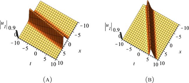
Figure 2. Evolution of the solution, equation ( |
8.1. Non-commutative case
We now discuss the non-commutative case. It has been shown in [13] that the behavior of matrix solitons differs from their scalar counterparts. Unlike scalar solitons, which keep their amplitudes unchanged during interactions, matrix solitons undergo transformations that depend on certain rules. These transformations affect the amplitudes, which are determined by vectors rather than individual values in the non-commutative setting. When considering the case of n = 1, we choose the solutions φ and χ of the Lax pair to be 2 × 2 matrices, given by 8.4 ), with each entry being a 2 × 2 matrix.
$\begin{eqnarray}\begin{array}{l}{\varphi }_{j}={{\rm{e}}}^{{\rm{i}}{\zeta }_{j}}{I}_{2},\ \quad {\chi }_{j}={{\rm{e}}}^{-{\rm{i}}{\zeta }_{j}}{I}_{2},\\ {\zeta }_{j}=-{\lambda }_{j}x+2{\lambda }_{j}^{2}(4\gamma \,{\lambda }_{j}^{2}-2{\lambda }_{j}{\alpha }_{1}-{\alpha }_{2})t.\end{array}\end{eqnarray}$
Here, I2 is the 2 × 2 identity matrix. And each entry in φ and χ and the constant matrix Q is a 2 × 2 matrix, so that these matrices are given by $\begin{eqnarray}\begin{array}{l}\varphi =\left(\begin{array}{cccc}{\varphi }_{1} & 0 & 0 & 0\\ 0 & {\varphi }_{1} & 0 & 0\end{array}\right),\ \chi =\left(\begin{array}{cccc}0 & 0 & {\chi }_{1} & 0\\ 0 & 0 & 0 & {\chi }_{1}\end{array}\right),\\ Q=\left(\begin{array}{cccc}{q}_{11} & {q}_{12} & {q}_{13} & {q}_{14}\\ {q}_{12} & {q}_{11} & {q}_{14} & {q}_{13}\\ {q}_{13} & {q}_{14} & {q}_{33} & {q}_{34}\\ {q}_{14} & {q}_{13} & {q}_{34} & {q}_{33}\end{array}\right).\end{array}\end{eqnarray}$
Therefore, the quasi-Gramian expression for u2 (which we will now denote as u1 for the non-commutative case) can be expressed as $\begin{eqnarray}\begin{array}{l}{u}^{1}=2{\rm{i}}\left(\begin{array}{cc}\left|\begin{array}{ccccc} & & {\rm{\Upsilon }}({\rm{\Xi }},\ Z) & & {\chi }^{11}\\ {\varphi }_{1} & 0 & 0 & 0 & \boxed{0}\end{array}\right| & \left|\begin{array}{ccccc} & & {\rm{\Upsilon }}({\rm{\Xi }},\ Z) & & {\chi }^{12}\\ {\varphi }_{1} & 0 & 0 & 0 & \boxed{0}\end{array}\right|\\ \left|\begin{array}{ccccc} & & {\rm{\Upsilon }}({\rm{\Xi }},\ Z) & & {\chi }^{11}\\ 0 & {\varphi }_{1} & 0 & 0 & \boxed{0}\end{array}\right| & \left|\begin{array}{ccccc} & & {\rm{\Upsilon }}({\rm{\Xi }},\ Z) & & {\chi }^{12}\\ 0 & {\varphi }_{1} & 0 & 0 & \boxed{0}\end{array}\right|\end{array}\right),\\ =2{\rm{i}}\left(\begin{array}{cc}{u}_{11} & {u}_{12}\\ {u}_{21} & {u}_{22}\end{array}\right),\,\mathrm{say},\end{array}\end{eqnarray}$
where ${\chi }^{11}={({q}_{13}{\chi }_{1}^{* }\ {q}_{14}{\chi }_{1}^{* }\ {q}_{33}{\chi }_{1}^{* }\ {q}_{34}{\chi }_{1}^{* })}^{\dagger },\ {\chi }^{12}={({q}_{14}{\chi }_{1}^{* }\ {q}_{13}{\chi }_{1}^{* }\ {q}_{34}{\chi }_{1}^{* }\ {q}_{33}{\chi }_{1}^{* })}^{\dagger }$ and ϒ(Ξ, Z) is the potential defined in equation (Within the context of a non-commutative system, the soliton solution, equation (8.11 ), is intricately influenced by both the spectral parameter λ and the elements composing the matrix Q. When specific entries, such as q13 and q14, are deliberately set to zero, the resulting solutions for u11, u12, u21, and u22 appear trivial. And where q13 = q14 = − 1, the graphical representations of solutions u11, u12, u21, and u22 manifest as a single consolidated plot instead of the originally intended four. Noteworthy is the fact that under these conditions, all solitons propagate with a consistent amplitude of 0.2163 units, as shown in figure 3. Unlike this symmetry, when q13 ≠ q14, the resulting graphs exhibit a variety of double- and single-peaked patterns for each component of the matrix u1 (see figure 4). It is worth highlighting that soliton u12 advances with an amplitude of 0.3860 units of large peak and 0.2317 units of small peak, while soliton u11 propagates with an amplitude of 1.9797 units. Additionally, an intriguing situation unfolds when we choose q12 = − q14 = − 2 and q11 = q13 = q33 = q34 = 0. For such parametric values, we notice a single-peaked soliton for u11 with an amplitude of 0.2214 units, while simultaneously observing a kink pattern in u12 of maximum height 0.8858 units (as seen in figure 5).
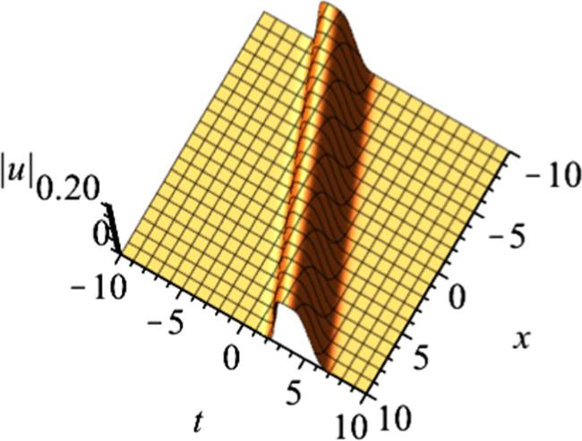
Figure 3. Evolution of the solution, equation ( |
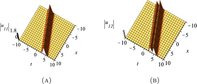
Figure 4. Evolution of the solution, equation ( |

Figure 5. Evolution of the solution, equation ( |
The solution, equation (8.11 ), includes several particular cases. When both α2 and γ are zero, the solution, equation (8.11 ), takes a different form. It becomes a solution of a non-commutative generalization of the complex modified KdV equation, and is further reduced to the standard modified KdV equation when the variable u is real-valued. Additionally, if we set γ to zero, we obtain the solution of the non-commutative extension of the Hirota equation. These solutions are depicted in figure 6. Furthermore, when we simultaneously set α1 and α2 to zero, we have the solution of the non-commutative LPD equation. Lastly, if we set α1 and γ to zero, we get the solution of non-commutative generalization of the NLS equation.

Figure 6. The profiles of u11 and u12 with γ = α2 = 0 in (A) and (B), and with γ = 0 in (C) and (D). All the other parameters are the same as in figure 5. |
In summary, studying the non-commutative version is important because it gives us different choices for arranging solitons. These arrangements depend not only on the spectral parameter λ but also on values in a matrix. Similarly, two soliton solutions for the non-commutative case are depicted in figures 7-9.
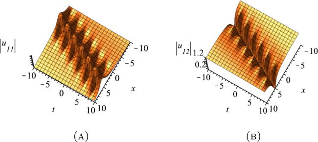
Figure 7. The profiles of uij, i, j = 1, 2 with α1 = 0.5, α2 = ν = 1, λ1 = 0.5i, λ2 = − 0.1 − 0.1i. All the other parameters are the same as in figure 5, (A) u11 profile, and (B) u12 profile. |

Figure 8. The profiles of uij, i, j = 1, 2 with α1 = 0.5, α2 = ν = 1, λ1 = 0.6i, λ2 = − 1.1 − 1.1i, (A) u11 profile, and (B) u12 profile. |

Figure 9. The profiles of uij, i, j = 1, 2 with α1 = 0.5, α2 = ν = 1, λ1 = 0.1 + 0.5i, λ2 = − 0.5i, (A) u11 profile, and (B) u12 profile. |
In figure 7, it is shown that solitons exhibiting breather-like structures are observed in the components u11 and u12, where (u11 ≠ u12). This occurrence can be attributed to the strength of the force acting between two solitons. When this force becomes sufficiently strong, solitons in a bound state have the ability to merge and transform into solitons with a breather-like structure. This phenomenon is commonly referred to as soliton fusion, which provides important insights into the dynamics of nonlinear wave systems by demonstrating the complicated behavior and complex interplay of solitons when exposed to strong interacting forces.
Figures 8-9 present a visual representation of two soliton solutions derived from the nc-HNLS equation. Within this context, solitons represent localized waves of energy that propagate through a medium with stability. The figures illustrate the interaction of two distinct solitons, each characterized by its own velocity, moving independently and later scattering without undergoing any shape changes. This behavior aligns with the defining characteristic of soliton robustness during interactions. Similarly, other multisoliton expressions can be obtained by repeatedly applying the DT to the seed solution. Note that we have omitted the explicit expression of soliton solutions for non-commutative cases as it is long and cumbersome.
9. Concluding remarks
This study explored the non-commutative extension of the HNLS equation. We have constructed Darboux and binary DTs and used these to obtain solutions in quasi-Wronskian and quasi-Gramian forms. These solutions were intricately linked to the nc-HNLS equation and its associated Lax pair. We demonstrated single- and double-peaked, kink, and bright solitons in non-commutative settings. Further, we also visualized the different types of interaction of two individual solitons: that is, two different lump energies moving at different velocities and frequencies that interact and scatter off without changing their profiles. The method proposed in this study serves as an effective tool, enabling the explicit construction of multi-solitons for other related non-commutative integrable systems.