In this paper, two types of fractional nonlinear equations in Caputo sense, time-fractional Newell–Whitehead equation (FNWE) and time-fractional generalized Hirota–Satsuma coupled KdV system (HS-cKdVS), are investigated by means of the q-homotopy analysis method (q-HAM). The approximate solutions of the proposed equations are constructed in the form of a convergent series and are compared with the corresponding exact solutions. Due to the presence of the auxiliary parameter h in this method, just a few terms of the series solution are required in order to obtain better approximation. For the sake of visualization, the numerical results obtained in this paper are graphically displayed with the help of Maple.
Di Liu, Qiongya Gu, Lizhen Wang. Q-homotopy analysis method for time-fractional Newell–Whitehead equation and time-fractional generalized Hirota–Satsuma coupled KdV system[J]. Communications in Theoretical Physics, 2024, 76(3): 035007. DOI: 10.1088/1572-9494/ad2364
1. Introduction
Fractional calculus, a generalization of classical calculus, was proposed by L'Hospital in 1695 and is more suitable than classical calculus for simulating some real-world problems. The advantages of the fractional differential operator are its nonlocality and ability to describe the memory effects of the system. Therefore, fractional calculus has attracted more and more attention in many applied fields, such as biology, physics, rheology, signal processing, electrochemistry [1–6], etc. It is well known that the construction of the exact solutions of fractional partial differential equations (FPDEs) is an important problem. Consequently, many scholars have introduced numerous methods to seek the solutions, such as the Lie symmetry analysis method [7–9], Adomian decomposition method [10], homotopy analysis transform method [11], Laplace transform collocation method [12], functional separation variables method [13], residual power series method [14], sub-equation method [15], homotopy perturbation method [16, 17], invariant subspace method [18], auxiliary function method [19, 20] and the classical Mittag-Leffler kernel [21].
An approach called the homotopy analysis method (HAM) was first proposed by Liao [22, 23] in 1992. The HAM forms a continuous mapping from the initial conjecture to the exact solution after selecting auxiliary linear operators. The HAM contains the auxiliary parameter to determine the convergence of the solution. Later, in 2012, the q-homotopy analysis method (q-HAM) was introduced by El-Tawil and Huseen in [24] and it is one of the most effective methods for solving nonlinear PDEs. It is actually an improvement of the embedding parameter q ∈ [0, 1] in the HAM to $q\in [0,\tfrac{1}{n}]$, n ≥ 1 appearing in the q-HAM. Moreover, the q-HAM contains the fractional factor that gives better convergence than the HAM. Recently, the method has been generalized and applied to some fractional PDEs, such as time-space fractional Fokker–Planck equations [25], time-fractional Ito equation and Sawada–Kotera equation [26], time-fractional Korteweg–de Vries and Korteweg–de Vries–Burgers equations [27] and time-space fractional gas dynamics equation [28].
In this paper, on the one hand, we consider the time-fractional Newell–Whitehead equation (FNWE) [29],
where 0 < α ≤ 1 is a parameter describing the order of the time-fractional derivative. Here and hereafter, ${{\rm{D}}}_{t}^{\alpha }u$ is the Caputo fractional differential operator with order α. Physically, to solve FPDEs, we need to specify additional conditions in order to produce a solution. Compared with other fractional operators, Caputo fractional operator has many advantages. First, its initial conditions have physical meaning. Second, the lower limit of integration in its definition can be arbitrarily selected and does not necessarily start from 0, which means that the reference interval can be freely regulated to make the equation have short-term memory. Third, the Caputo fractional derivative of a constant is 0. Equation (1) can be considered as a generalization of the Newell–Whitehead equation (NWE). The NWE can simulate the interaction between the effect of the diffusion term and the nonlinear effect of the reaction term. Function u is denoted as the distribution of temperature in an infinitely thin and long rod or as the flow rate of a fluid in an infinitely long pipe with a small diameter [30, 31]. The NWE has been widely used in mechanical, chemical and bio-engineering. Furthermore, some approaches, such as the reduced differential transform method [32], Adomian decomposition methods [33] and variational iteration method [34], have been developed to solve the FNWE.
On the other hand, we consider the following time-fractional generalized Hirota–Satsuma coupled KdV system (HS-cKdVS):
The generalized HS-cKdVS describes the interaction between long waves with different dispersion relations [35]. In this system, u(x, t), v(x, t) and w(x, t) are the amplitude of the wave modes as functions of space variable x and time variable t. Recently, some researchers have investigated this system using different methods. Abbasbandy studied the approximate analytical solution of the generalized HS-cKdVS via the homotopy analysis method [36]. Prakash and Verma [37] employed q-homotopy analysis Sumudu transform method and residual power series method to find the analytical solution of system (2). Some exact solutions of system (2) were constructed by Saberi and Hejazi using the invariant subspace method with Caputo sense [38]. Martínez, Reyes and Sosa [39] obtained the analytical solutions by applying the sub-equation method for the time-space fractional generalized HS-cKdVS.
In this paper, we have applied the q-HAM to solve the time FNWE and the time-fractional generalized HS-cKdVS with different initial conditions, because it is too difficult to find the exact solution of the two equations, and the proposed method can be used to find the approximate solution of these two equations, which is helpful for a deeper understanding of the proposed equations at a later stage. Keeping the above facts in mind, this paper is the first study to investigate the approximate solutions of the time FNWE and the time-fractional generalized HS-cKdVS with the help of the q-HAM.
The rest of the study is set out as follows. Some basic definitions and formulas related to fractional calculus are provided in section 2. The basic definition of the q-HAM is introduced in section 3. In section 4, we intend to use the q-HAM to solve equation (1) and system (2). We conclude this paper in section 5.
2. Preliminaries
In this section, we introduce some definitions and formulas related to fractional calculus, which will be used throughout the paper.
[1] The Riemann–Liouville fractional integral operator of order α of function f(t) is given as,
Consider the nonlinear fractional differential equation of the form,
$\begin{eqnarray}{ \mathcal N }[{{\rm{D}}}_{t}^{\alpha }u(x,t)]-f(x,t)=0,\end{eqnarray}$
where ${ \mathcal N }$ is a nonlinear operator, ${{\rm{D}}}_{t}^{\alpha }$ denotes the Caputo fractional derivative, (x, t) are independent variables, f(x, t) is the given function, while u(x, t) is an unknown function. Construct the zeroth-order deformation equation as follows:
$\begin{eqnarray}\begin{array}{l}(1-{nq}){\mathfrak{L}}[\varphi (x,t;q)-{u}_{0}(x,t)]\\ \,=\,{qhH}(x,t)({ \mathcal N }[{{\rm{D}}}_{t}^{\alpha }\varphi (x,t;q)]-f(x,t)),\end{array}\end{eqnarray}$
where n ≥ 1, $q\in [0,\tfrac{1}{n}]$ is called an embedded parameter, h ≠ 0 is an auxiliary parameter, H(x, t) is a non-zero auxiliary function, ${\mathfrak{L}}$ is an auxiliary linear operator and u0(x, t) is the initial guess of u(x, t). Clearly, when q = 0 and $q=\tfrac{1}{n}$, we can obtain the following result:
respectively. Thus, as q rises from 0 to $\tfrac{1}{n}$, the solution φ(x, t; q) ranges from the initial guess u0(x, t) to the solution u(x, t). Assume that u0(x, t), ${\mathfrak{L}}$, h and H(x, t) are appropriately selected so that the solution φ(x, t; q) of equation (6) exists for $q\in [0,\tfrac{1}{n}]$. The expansion of the function φ(x, t; q) in Taylor series form gives:
Differentiating zeroth-order deformation equation (6) m times with respect to the embedding parameter q, setting q = 0 and dividing them by m!, we can derive the following mth-order deformation equation:
It needs to be emphasized that ${u}_{m}(x,t)$ for $m\geqslant 1$ is controlled by the linear equation (12) with linear boundary conditions from the original problem. The presence of factor ${\left(\tfrac{1}{n}\right)}^{m}$ can produce more opportunities for convergence and even better and faster convergence than the standard HAM. In particular, when $\alpha =1$ and n = 1 in equation (6), the standard HAM can be achieved.
The convergence and error analysis of the q-HAM are discussed in the following theorems, which shows that the convergence of the q-HAM is more accurate than the convergence of the HAM.
[40] If the nonlinear operator is preserved on the power series in q, the solution of equation (6) together with equation (5) exists as a power series in the following:
[40] Consider a Banach space $(A,\parallel \cdot \parallel )$ with $A\subset {\mathbb{R}}$. Suppose that the initial estimation ${u}_{0}(x,t)$ remains inside the ball of the solution $u(x,t)$. Let r be a constant, then for a prescribed value of h and $0\lt r\lt n$, if for all k,
Then, the series solution ${\sum }_{k=0}^{\infty }{U}_{k}{(t,n)={\sum }_{k\,=\,0}^{\infty }{u}_{k}(t)\left(\tfrac{1}{n}\right)}^{k}$ is convergent on the zone of definition t.
[41] Assume that the truncated series ${\sum }_{k=0}^{p}{u}_{k}{(x,t)\left(\tfrac{1}{n}\right)}^{k}$ is used as an approximation to the solution $u(x,t).$ If there exists a constant $0\lt l\lt 1$ satisfying $\parallel {u}_{m+1}(x,t)\parallel \leqslant l\parallel {u}_{m}(x,t)\parallel $, then the maximum absolute truncated error is determined as,
In this section, the q-HAM is used to construct the analytical solutions of time FNWEs and time-fractional generalized HS-cKdVS to verify the effectiveness of the previous q-HAM algorithm. The results of this study are graphed by Maple.
4.1. The time-fractional Newell–Whitehead equation
In this section, we construct the series solutions of time FNWE (1) with two different initial conditions with the help of the q-HAM.
Consider the time FNWE (1) and its initial condition is given as follows:
Proceeding in similar steps, the remaining iterations um(x, t) (m = 3, 4, 5, …) can be obtained. Therefore, the series solution of equations (1) and (17) obtained by the q-HAM is
Equation (26) is the appropriate solution to equations (1) and (17) in terms of convergence parameters h and n. Moreover, choosing n = 1, α = 1 and h = − 1, the series solution ${\sum }_{m=1}^{N}{u}_{m}{(x,t)\left(\tfrac{1}{n}\right)}^{m}$ of equations (1) and (17) converges to its exact solution [34] as N → ∞ :
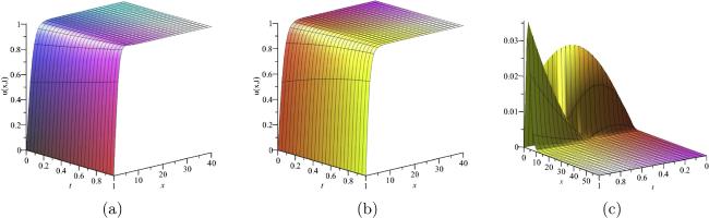
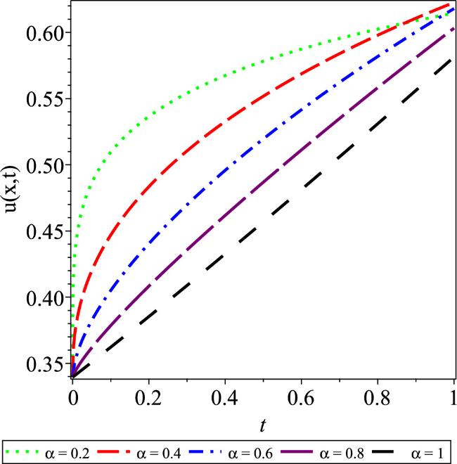
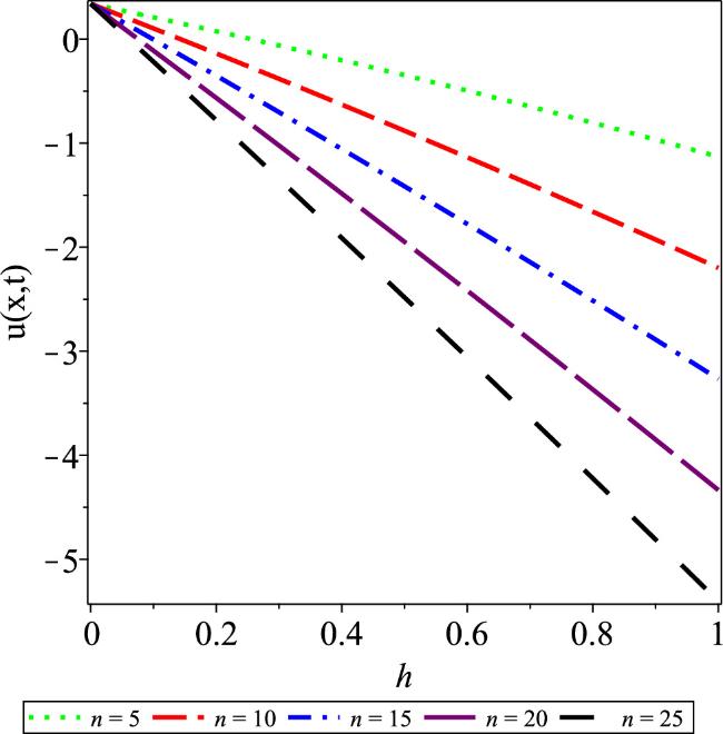
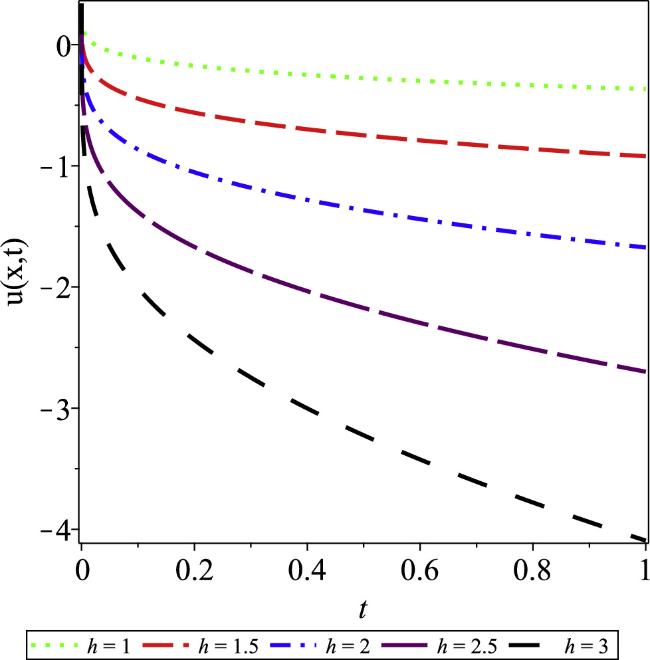
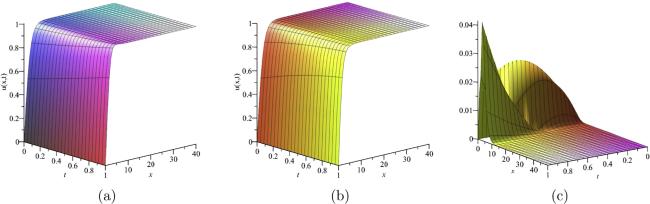
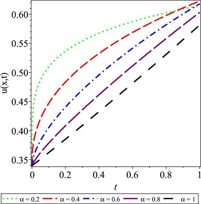
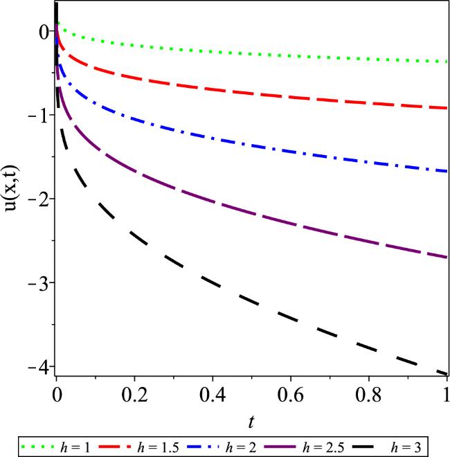
With the help of the 3D plots, we demonstrate the wave propagation pattern of the wave along the x-axis. Figure 1 presents the plots of the approximate solution, exact solution and absolute error when h = − 0.44, n = 1 and α = 1 for equations (1) and (17). It is worth pointing out that the numerical solution obtained by the q-HAM and the exact solution u(x, t) are almost identical in figures 1(a) and (b). Figure 2 displays the behavior of the flow velocity u(x, t) for distinct values of α at x = 1, h = − 1 and n = 1. We note that the q-HAM solution increases with the increase in t in figure 2. Figure 3 exhibits the behavior of the flow velocity u(x, t) for different values of n at x = 1, h = − 1 and α = 0.2. It can be seen from figure 3 that as the values of h increase, the q-HAM solution u(x, t) decreases. In figure 4, different values of the convergence control parameter h are selected to minimize residual error and guarantee the convergence of the series solution by choosing the appropriate value of h.
Equation (31) is the appropriate solution to equations (1) and (28) in terms of convergence parameters h and n. Moreover, when n = 1, α = 1 and h = − 1, the series solution ${\sum }_{m=1}^{N}{u}_{m}{(x,t)\left(\tfrac{1}{n}\right)}^{m}$ of equations (1) and (28) converges to its exact solution [34] as N → ∞ :
The wave propagation pattern of the wave along the x-axis can be seen from the 3D plots. Figure 5 gives the plots of the approximate solution, exact solution and absolute error when h = − 0.45, n = 1 and α = 1 for equations (1) and (28). It can be observed that the numerical solution obtained by the q-HAM and the exact solution u(x, t) are consistent with each other in figures 5(a) and (b). Figure 6 demonstrates the behavior of the flow velocity u(x, t) for distinct values of α at x = 1, h = − 1 and n = 1 and indicates that the q-HAM solution increases with the increase in α. Figure 7 displays the behavior of the flow velocity u(x, t) for different values of n at x = 1, h = − 1 and α = 0.2. It is clear from figure 7 that as the values of h increase, the q-HAM solution u(x, t) decreases. In figure 8, different values of the convergence control parameter h are selected to minimize residual error.
Moreover, we can repeat the above process to deduce the formulas of um(x, t), vm(x, t) and wm(x, t) (m = 3, 4, 5, …) and deduce the following series solution of system (2):
Eq. (42) is the appropriate solution to system (2) in terms of convergence parameters h and n. Furthermore, taking n = 1, h = − 1 and α = 1, the series solutions ${\sum }_{m=1}^{N}{u}_{m}{(x,t)\left(\tfrac{1}{n}\right)}^{m}$, ${\sum }_{m=1}^{N}{v}_{m}{(x,t)\left(\tfrac{1}{n}\right)}^{m}$ and ${\sum }_{m=1}^{N}{w}_{m}{(x,t)\left(\tfrac{1}{n}\right)}^{m}$ of system (2) converge to its soliton solution [35] as N → ∞ :
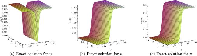
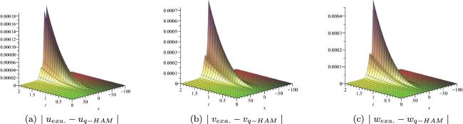
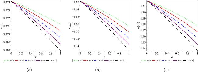
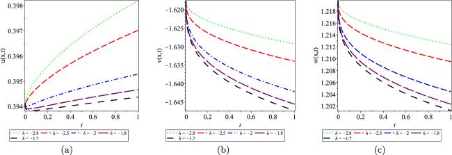
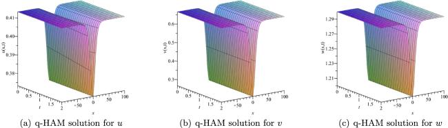
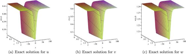
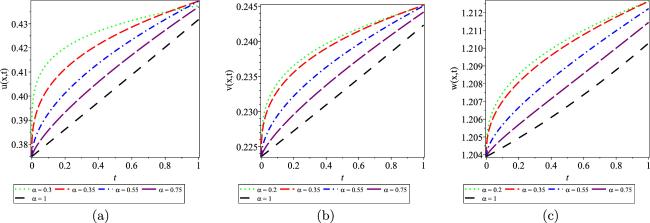
Figures 9–11 show the plots of the approximate solution, exact solution and absolute error when h = − 1, n = 1, α = 1, c0 = β = 1.2 and c1 = k = 0.1 for system (2) with the initial conditions (33), respectively. The numerical solution obtained by the q-HAM is almost similar to the exact solution, as observed in figures 9 and figure 10. The effect of the various parameters and variables on the amplitude of the wave modes is shown from figures 12–14. Figure 12 presents the behavior of the numerical solution for distinct values of α at x = 2, h = − 1 and n = 2. It is easy to see that the q-HAM solution increases with increasing t in figure 12. Figure 13 exhibits the behavior for different values of n at x = 2 and α = 0.3. We note from figure 13 that as the values of h increase, the q-HAM solution decreases. In figure 14, diverse values of the convergence control parameter h are selected to lessen the error.
In the same way, um(x, t), vm(x, t) and wm(x, t) (m = 3, 4, 5, …) can be derived. Accordingly, the series solution of system (2) by the q-HAM in series form is provided as follows:
Equation (50) is the appropriate solution to system (2) in terms of convergence parameters h and n. In addition, for n = 1, h = − 1 and α = 1, the series solution ${\sum }_{m=1}^{N}{u}_{m}{(x,t)\left(\tfrac{1}{n}\right)}^{m}$, ${\sum }_{m=1}^{N}{v}_{m}{(x,t)\left(\tfrac{1}{n}\right)}^{m}$ and ${\sum }_{m=1}^{N}{w}_{m}{(x,t)\left(\tfrac{1}{n}\right)}^{m}$ converges to soliton solution [35] of system (2) as N → ∞ :
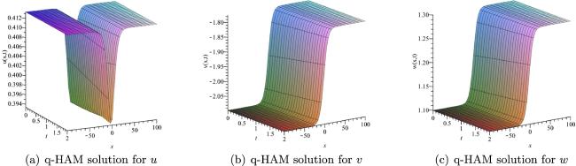
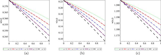
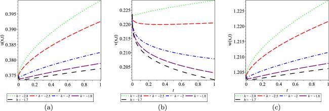
Figures 15–17 display the plots of the approximate solution, exact solution and absolute error when h = − 1, n = 1, α = 1, c0 = β = 1.2 and c1 = k = 0.1 for system (2) with the initial conditions (44), respectively. As can easily be discovered from figures 15 and 16, the numerical solution obtained by the q-HAM coincides with the exact solution. Figures 18–20. show the effect of the various parameters and variables on the amplitude of the wave modes. Figure 18 depicts the behavior of the numerical solution for distinct values of α at x = 2, h = − 1 and n = 2. It is realized that the q-HAM solution increases with the increase in t in figure 18. Figure 19 exhibits the behavior of the numerical solution for diverse values of n at x = 2 and α = 0.3. It can be seen from figure 19 that as the values of h increase, the q-HAM solution decreases. In figure 20, different values of the convergence control parameter h are selected to minimize residual error and guarantee the convergence of the series solution by choosing the appropriate value of h.
Figure 18. Plots of u(x, t), v(x, t) and w(x, t) for Ex. 4.4. with fixed c0 = β = 1.2, c1 = k = 0.1, x = 2, n = 1, and h = − 1 at different values of α.
Figure 20. Plots of h curves for Ex. 4.4. at c0 = β = 1.2, c1 = k = 0.1, x = n = 2 and α = 0.3 with increasing values of t.
5. Conclusion
In this present study, the new approximate solutions of the time FNWE and the time-fractional generalized HS-cKdVS are successfully constructed by means of the q-HAM. The results show that the q-HAM gives the solution in the form of a convergent series without using linearization and perturbation. In addition, it is shown from the absolute truncated error image that the results of the present method are in excellent agreement with the exact solution. The auxiliary parameter h and n(n ≥ 1) used in the proposed method describe the nonlocal convergence. Therefore, the investigation of this paper shows that the q-HAM is an effective and powerful tool to solve nonlinear FPDEs with the sense of Caputo derivative.
Funding
This study is supported by the National Natural Science Foundation of China (Grant No. 12 271 433).
Conflict of Interest
The authors declare that they have no conflicts of interest.
MillerK SRossB1993An introduction to the fractional calculus and fractional differential equations Wiley
2
HilferR2000Applications of fractional calculus in physics World Scientific
3
KumarS et al 2024 Numerical investigations on COVID-19 model through singular and non-singular fractional operators Numer. Meth. Part. D. E.40 e22707
4
YavuzM et al 2021 Analysis and numerical computations of the fractional regularized long-wave equation with damping term Math. Methods Appl. Sci.44 7538-7555
GuQWangLYangY2022 Group Classifications, optimal Systems, symmetry reductions and conservation law of the generalized fractional porous medium equation Commun. Nonlinear Sci.115 106712
ChengXWangL2021 Invariant analysis, exact solutions and conservation laws of (2+1)-dimensional time fractional Navier–Stokes equations Proc. R. Soc. A-Math. Phys. Eng. Sci.477 20210220
YangYWangL2022 Lie symmetry analysis, conservation laws and separation variable type solutions of the time-fractional porous medium equation Waves Random Complex Media32 980-999
KumarS et al 2020 A modified analytical approach with existence and uniqueness for fractional Cauchy reaction-diffusion equations Adv. Differ. Equ-NY28 1-18
ModanliMKoksalM E2022 Laplace transform collocation method for telegraph equations defined by Caputo derivative Math. Model Numer. Simulat. Appl.2 177-186
DururHYokuşAYavuzM2022 Behavior analysis and asymptotic stability of the traveling wave solution of the Kaup–Kupershmidt equation for conformable derivative Fract. Calc. New Appl. Underst. Nonlinear Phenom.3 162
16
El-DibY O2021 Homotopy perturbation method with rank upgrading technique for the superior nonlinear oscillation Math. Comput. Simulat.182 555-565
JleliM et al 2019 Analytical approach for time fractional wave equations in the sense of Yang–Abdel–Aty–Cattani via the homotopy perturbation transform method Alex. Eng. J.59 2858-2863
KumarS et al 2021 A fractional model for population dynamics of two interacting species by using spectral and Hermite wavelets methods Numer. Meth. Part. D. E.37 1652-1672
DuranS et al 2023 Discussion of numerical and analytical techniques for the emerging fractional order Murnaghan model in materials science Opt. Quant. Electron.55 571
YavuzM2022 European option pricing models described by fractional operators with classical and generalized Mittag-Leffler kernels Numer. Meth. Part. D. E.38 434-456
SaadK MAL-ShareefE HAlomariA KDumitruBGómez-AguilarJ F2020 On exact solutions for time-fractional Korteweg–de Vries and Korteweg–de Vries–Burger's equations using homotopy analysis transform method Chin. J. Phys.63 149-162
AasaraaiA2011 Analytic solution for Newell–Whitehead–Segel Equation by differential transform method, Middle East J. Sci. Res.10 270-273
30
Macías-DíazJ ERuiz-RamírezJ2011 A non-standard symmetry-preserving method to compute bounded solutions of a generalized Newell–Whitehead–Segel equation Appl. Numer. Math.61 630-640
MohamedM SAl-QarshiT T2021 Approximate solutions for the time-space fractional nonlinear of partial differential equations using reduced differential transform method Int. J. Computer Appl. Math.2 16
33
MohamedS MAl-MalkiFTalibRTaifS A2013 Approximate analytical and numerical solutions to fractional Newell–Whitehead equation by fractional complex transform Int. J. Appl. Math.26 657-669
Yépez-MartínezHReyesJ MSosaI O2014 Fractional sub-equation method and analytical solutions to the Hirota–Satsuma coupled KdV equation and coupled mKdV equation J. Adv. Math. Computer Sci.4 572
PrakashAKumarMBaleanuD2018 A new iterative technique for a fractional model of nonlinear Zakharov–Kuznetsov equations via Sumudu transform Appl. Math. Comput.334 30-40
ArifeA SVananiS KYildirimA2011 Numerical solution of Hirota–Satsuma coupled Kdv and a coupled MKdv equation by means of homotopy analysis method World Appl. Sci. J.13 2271-2276


