Welcome to visit Communications in Theoretical Physics,
Quantum Physics and Quantum Information

Tighter sum uncertainty relations via (α, β, γ) weighted Wigner-Yanase-Dyson skew information

  • Cong Xu 1 ,
  • Zhaoqi Wu , 2, ,
  • Shao-Ming Fei , 1, 3,
Expand
  • 1School of Mathematical Sciences, Capital Normal University, Beijing 100048, China
  • 2Department of Mathematics, Nanchang University, Nanchang 330031, China
  • 3 Max-Planck-Institute for Mathematics in the Sciences, 04103 Leipzig, Germany

Authors to whom any correspondence should be addressed.

Received date: 2023-09-28

  Revised date: 2024-01-21

  Accepted date: 2024-01-23

  Online published: 2024-03-06

Copyright

© 2024 Institute of Theoretical Physics CAS, Chinese Physical Society and IOP Publishing

Abstract

We establish tighter uncertainty relations for arbitrary finite observables via (α, β, γ) weighted Wigner–Yanase–Dyson ((α, β, γ) WWYD) skew information. The results are also applicable to the (α, γ) weighted Wigner–Yanase–Dyson ((α, γ) WWYD) skew information and the weighted Wigner–Yanase–Dyson (WWYD) skew information. We also present tighter lower bounds for quantum channels and unitary channels via (α, β, γ) modified weighted Wigner–Yanase–Dyson ((α, β, γ) MWWYD) skew information. Detailed examples are provided to illustrate the tightness of our uncertainty relations.

Cite this article

Cong Xu , Zhaoqi Wu , Shao-Ming Fei . Tighter sum uncertainty relations via (α, β, γ) weighted Wigner-Yanase-Dyson skew information[J]. Communications in Theoretical Physics, 2024 , 76(3) : 035102 . DOI: 10.1088/1572-9494/ad216b

1. Introduction

As one of the cornerstones of quantum mechanics, the uncertainty principle reveals the insights that distinguish quantum theory from classical theory. Heisenberg [1] originally proposed the uncertainty principle in 1927, which indicates that the position and momentum of a particle cannot be precisely determined simultaneously. Robertson [2] generalized the variance-based uncertainty relation for position and momentum to arbitrary two observables A and B.
$\begin{eqnarray}{\rm{\Delta }}A{\rm{\Delta }}B\geqslant \displaystyle \frac{1}{2}| \langle \psi | [A,B]| \psi \rangle | ,\end{eqnarray}$
where [A, B] = ABBA and ${\rm{\Delta }}M=\sqrt{\langle \psi | {M}^{2}| \psi \rangle -\langle \psi | M| \psi {\rangle }^{2}}$ is the standard deviation of the observable M with respect to a fixed state ∣ψ⟩.
The uncertainty principle has attracted sustained attention. A host of methods have been presented to characterize the uncertainty [316]. The skew information is one of the typical ways to describe the uncertainty principle. The skew information of an observable A with respect to a quantum state ρ is given by [17].
$\begin{eqnarray}{{\rm{I}}}_{\rho }(A)=-\displaystyle \frac{1}{2}\mathrm{Tr}\left({\left[\sqrt{\rho },A\right]}^{2}\right)=\displaystyle \frac{1}{2}{\parallel \left[\sqrt{\rho },A\right]\parallel }^{2},\end{eqnarray}$
which is called the Wigner–Yanase (WY) skew information. Later, Dyson proposed a one-parameter extension of the WY skew information, called Wigner–Yanase–Dyson (WYD) skew information. In [18] the WYD skew information is further generalized to the generalized Wigner–Yanase–Dyson (GWYD) skew information. The corresponding definitions of the above-mentioned skew information for arbitrary (not necessarily Hermitian) operators have also been introduced [9, 10, 19, 20]. The uncertainty relation related to WY skew information was initially introduced by Luo [21]. Recently, uncertainty relations based on various generalized skew information have been explored intensely in [19, 20, 2230].
By considering the arithmetic mean of ρα and ρ1−α, Furuichi et al [31] introduced another one-parameter skew information,
$\begin{eqnarray}\begin{array}{rcl}{{\rm{K}}}_{\rho }^{\alpha }(A) & = & -\displaystyle \frac{1}{2}\mathrm{Tr}\left({\left[\displaystyle \frac{{\rho }^{\alpha }+{\rho }^{1-\alpha }}{2},A\right]}^{2}\right)\\ & = & \displaystyle \frac{1}{2}{\parallel \left[\displaystyle \frac{{\rho }^{\alpha }+{\rho }^{1-\alpha }}{2},A\right]\parallel }^{2},\,0\leqslant \alpha \leqslant 1,\end{array}\end{eqnarray}$
which is called the weighted Wigner–Yanase–Dyson (WWYD) skew information [20]. A generalization of equation (3) was presented in [32] for an arbitrary operator E,
$\begin{eqnarray}\begin{array}{rcl}{{\rm{K}}}_{\rho }^{\alpha }(E) & = & -\displaystyle \frac{1}{2}\mathrm{Tr}\left(\left[\displaystyle \frac{{\rho }^{\alpha }+{\rho }^{1-\alpha }}{2},{E}^{\dagger }\right]\left[\displaystyle \frac{{\rho }^{\alpha }+{\rho }^{1-\alpha }}{2},E\right]\right)\\ & = & \displaystyle \frac{1}{2}{\parallel \left[\displaystyle \frac{{\rho }^{\alpha }+{\rho }^{1-\alpha }}{2},E\right]\parallel }^{2},\,0\leqslant \alpha \leqslant 1,\end{array}\end{eqnarray}$
which is termed as the modified weighted Wigner–Yanase–Dyson (MWWYD) skew information in [20]. Note that equation (4) reduces to equation (14) in [9], and equation (3) reduces to equation (2) when $\alpha =\tfrac{1}{2}$, respectively.
Recently, the two-parameter extension of equation (3) was introduced in [33],
$\begin{eqnarray}\begin{array}{rcl}{{\rm{K}}}_{\rho ,\gamma }^{\alpha }(A) & = & -\displaystyle \frac{1}{2}\mathrm{Tr}\left({[(1-\gamma ){\rho }^{\alpha }+\gamma {\rho }^{1-\alpha },A]}^{2}\right)\\ & = & \displaystyle \frac{1}{2}{\parallel \left[(1-\gamma ){\rho }^{\alpha }+\gamma {\rho }^{1-\alpha },A\right]\parallel }^{2},\\ & & 0\leqslant \alpha \leqslant 1\,,\,0\leqslant \gamma \leqslant 1,\end{array}\end{eqnarray}$
which is called the (α, γ) weighted Wigner–Yanase–Dyson ((α, γ) WWYD) skew information in [34].
Motivated by the equation (5) above and equation (3) in [19], we introduced the (α, β, γ) weighted Wigner–Yanase–Dyson ((α, β, γ) WWYD) skew information [35],
$\begin{eqnarray}\begin{array}{rcl}{{\rm{K}}}_{\rho ,\gamma }^{\alpha ,\beta }(A) & = & -\displaystyle \frac{1}{2}\mathrm{Tr}\left({\left[(1-\gamma ){\rho }^{\alpha }+\gamma {\rho }^{\beta },A\right]}^{2}{\rho }^{1-\alpha -\beta }\right)\\ & = & \displaystyle \frac{1}{2}{\parallel \left[(1-\gamma ){\rho }^{\alpha }+\gamma {\rho }^{\beta },A\right]{\rho }^{\displaystyle \frac{1-\alpha -\beta }{2}}\parallel }^{2},\\ & & \alpha ,\beta \geqslant 0,\,\alpha +\beta \leqslant 1,0\leqslant \gamma \leqslant 1,\end{array}\end{eqnarray}$
and its non-Hermitian extension, the (α, β, γ) modified weighted Wigner–Yanase–Dyson ((α, β, γ) MWWYD) skew information [35],
$\begin{eqnarray}\begin{array}{rcl}{{\rm{K}}}_{\rho ,\gamma }^{\alpha ,\beta }(E) & = & -\displaystyle \frac{1}{2}\mathrm{Tr}\left([(1-\gamma ){\rho }^{\alpha }+\gamma {\rho }^{\beta },{E}^{\dagger }]\right.\\ & & \left.\times \,[(1-\gamma ){\rho }^{\alpha }+\gamma {\rho }^{\beta },E]{\rho }^{1-\alpha -\beta }\right)\\ & = & \displaystyle \frac{1}{2}{\parallel \left[(1-\gamma ){\rho }^{\alpha }+\gamma {\rho }^{\beta },E\right]{\rho }^{\displaystyle \frac{1-\alpha -\beta }{2}}\parallel }^{2},\\ & & \alpha ,\beta \geqslant 0,\,\alpha +\beta \leqslant 1,0\leqslant \gamma \leqslant 1.\end{array}\end{eqnarray}$
Here equation (7) reduces to equation (7) in [35] and equation (6) reduces to equation (5) when β = 1 − α, respectively.
As the broadest form of measurement [36, 37], quantum channels play a crucial role in quantum theory. Chen et al [38] investigated the summation form of the uncertainty relations based on WY skew information for observables. Fu et al [39] explored the uncertainty relations for quantum channels in terms of WY skew information. Recently, the summation form of the uncertainty relations associated with skew information for arbitrary finite quantum observables and quantum channels has also been derived [4045].
The paper is structured as follows. In section 2, by using operator norm inequalities, new uncertainty relations of observables are given in terms of the (α, β, γ) WWYD skew information. We present two distinct types of uncertainty relations for quantum channels with respect to the (α, β, γ) MWWYD skew information and establish an optimal lower bound in section 3. The tighter uncertainty relations of unitary channels are presented in section 4. We conclude with a summary in section 5.

2. Sum uncertainty relations for arbitrary finite N observables

For arbitrary finite N observables A1, A2, ⋯ ,AN, Xu et al [34] provided the following sum uncertainty relations,
$\begin{eqnarray}\begin{array}{rcl} & & \displaystyle \sum _{i=1}^{N}{{\rm{K}}}_{\rho ,\gamma }^{\alpha ,\beta }({A}_{i})\geqslant \displaystyle \frac{1}{N-2}\left[\displaystyle \sum _{1\leqslant i\lt j\leqslant N}{{\rm{K}}}_{\rho ,\gamma }^{\alpha ,\beta }({A}_{i}+{A}_{j})\right.\\ & & \left.-\displaystyle \frac{1}{{\left(N-1\right)}^{2}}{\left(\displaystyle \sum _{1\leqslant i\lt j\leqslant N}\sqrt{{{\rm{K}}}_{\rho ,\gamma }^{\alpha ,\beta }({A}_{i}+{A}_{j})}\right)}^{2}\right],\end{array}\end{eqnarray}$
$\begin{eqnarray}\begin{array}{rcl} & & \displaystyle \sum _{i=1}^{N}{{\rm{K}}}_{\rho ,\gamma }^{\alpha ,\beta }({A}_{i})\geqslant \displaystyle \frac{1}{N}{{\rm{K}}}_{\rho ,\gamma }^{\alpha ,\beta }\left(\displaystyle \sum _{i=1}^{N}{A}_{i}\right)\\ & & +\displaystyle \frac{2}{\left.{N}^{2}(N-1\right)}{\left(\displaystyle \sum _{1\leqslant i\lt j\leqslant N}\sqrt{{{\rm{K}}}_{\rho ,\gamma }^{\alpha ,\beta }({A}_{i}-{A}_{j})}\right)}^{2}\,,\end{array}\end{eqnarray}$
and
$\begin{eqnarray}\begin{array}{rcl}\displaystyle \sum _{i=1}^{N}{{\rm{K}}}_{\rho ,\gamma }^{\alpha ,\beta }({A}_{i}) & \geqslant & \mathop{\max }\limits_{x\in \{0,1\}}\displaystyle \frac{1}{2(N-1)}\\ & & \times \,\left[\displaystyle \frac{2}{N(N-1)}{\left(\displaystyle \sum _{1\leqslant i\lt j\leqslant N}\sqrt{{{\rm{K}}}_{\rho ,\gamma }^{\alpha ,\beta }\left({A}_{i}+{\left(-1\right)}^{x}{A}_{j}\right)}\right)}^{2}\right.\\ & & \left.+\displaystyle \sum _{1\leqslant i\lt j\leqslant N}{{\rm{K}}}_{\rho ,\gamma }^{\alpha ,\beta }({A}_{i}+{\left(-1\right)}^{x+1}{A}_{j})\right],\end{array}\end{eqnarray}$
where α, β ≥ 0, α + β ≤ 1, 0 ≤ γ ≤ 1, N > 2 for the inequality (8) and N ≥ 2 for the inequalities (910). For convenience we denote by Lb1, Lb2 and Lb3 the right-hand sides of (8), (9) and (10), respectively.
The following relations are given in the appendix B in [45],
$\begin{eqnarray}\begin{array}{rcl}\displaystyle \sum _{i=1}^{N}\parallel {u}_{i}{\parallel }^{2} & \geqslant & \displaystyle \frac{1}{{MN}+(N-2)L}\\ & & \times \,\left\{\displaystyle \frac{2L}{N(N-1)}{\left(\displaystyle \sum _{1\leqslant i\lt j\leqslant N}\parallel {u}_{i}+{u}_{j}\parallel \right)}^{2}\right.\\ & & +\,\left.M\displaystyle \sum _{1\leqslant i\lt j\leqslant N}\parallel {u}_{i}-{u}_{j}{\parallel }^{2}+(M-L){\parallel \displaystyle \sum _{i=1}^{N}{u}_{i}\parallel }^{2}\right\},\end{array}\end{eqnarray}$
for ML > 0,
$\begin{eqnarray}\begin{array}{rcl}\displaystyle \sum _{i=1}^{N}\parallel {u}_{i}{\parallel }^{2} & \geqslant & \displaystyle \frac{1}{{MN}+(N-2)L}\\ & & \times \,\left\{\displaystyle \frac{2M}{N(N-1)}{\left(\displaystyle \sum _{1\leqslant i\lt j\leqslant N}\parallel {u}_{i}-{u}_{j}\parallel \right)}^{2}\right.\\ & & +\,\left.L\displaystyle \sum _{1\leqslant i\lt j\leqslant N}\parallel {u}_{i}+{u}_{j}{\parallel }^{2}+(M-L){\parallel \displaystyle \sum _{i=1}^{N}{u}_{i}\parallel }^{2}\right\},\end{array}\end{eqnarray}$
for LM > 0,
$\begin{eqnarray}\begin{array}{rcl}\displaystyle \sum _{i=1}^{N}\parallel {u}_{i}{\parallel }^{2} & \geqslant & \displaystyle \frac{1}{{MN}+(N-2)L}\\ & & \,\times \,\left\{\displaystyle \frac{M-L}{{\left(N-1\right)}^{2}}{\left(\displaystyle \sum _{1\leqslant i\lt j\leqslant N}\parallel {u}_{i}+{u}_{j}\parallel \right)}^{2}\right.\\ & & +\,\left.M\displaystyle \sum _{1\leqslant i\lt j\leqslant N}\parallel {u}_{i}-{u}_{j}{\parallel }^{2}+L\displaystyle \sum _{1\leqslant i\lt j\leqslant N}\parallel {u}_{i}+{u}_{j}{\parallel }^{2}\right\}\end{array}\end{eqnarray}$
for arbitrary L > M > 0. By replacing ui and uj with $\left[(1-\gamma ){\rho }^{\alpha }+\gamma {\rho }^{\beta },{A}_{i}\right]{\rho }^{\tfrac{1-\alpha -\beta }{2}}$ and $\left[(1-\gamma ){\rho }^{\alpha }+\gamma {\rho }^{\beta },{A}_{j}\right]{\rho }^{\tfrac{1-\alpha -\beta }{2}}$, respectively, in the above inequalities, we obtain the following inequalities.

For arbitrary finite N observables ${A}_{1},{A}_{2},\cdots ,{A}_{N}$ ($N\geqslant 2$), we have the following sum uncertainty relation via $(\alpha ,\beta ,\gamma )$ WWYD skew information,

$\begin{eqnarray}\begin{array}{l}\displaystyle \sum _{i=1}^{N}{{\rm{K}}}_{\rho ,\gamma }^{\alpha ,\beta }({A}_{i})\geqslant \max \{{\overline{{Lb}}}_{1},{\overline{{Lb}}}_{2},{\overline{{Lb}}}_{3}\},\end{array}\end{eqnarray}$
where
$\begin{eqnarray}\begin{array}{rcl}{\overline{{Lb}}}_{1} & = & \displaystyle \frac{1}{{MN}+(N-2)L}\\ & & \times \,\left\{\displaystyle \frac{2L}{N(N-1)}{\left(\displaystyle \sum _{1\leqslant i\lt j\leqslant N}\sqrt{{{\rm{K}}}_{\rho ,\gamma }^{\alpha ,\beta }({A}_{i}+{A}_{j})}\right)}^{2}\right.\\ & & +\,\left.M\displaystyle \sum _{1\leqslant i\lt j\leqslant N}{{\rm{K}}}_{\rho ,\gamma }^{\alpha ,\beta }({A}_{i}-{A}_{j})+(M-L){{\rm{K}}}_{\rho ,\gamma }^{\alpha ,\beta }\left(\displaystyle \sum _{i=1}^{N}{A}_{i}\right)\right\},\end{array}\end{eqnarray}$
$\begin{eqnarray}\begin{array}{rcl}{\overline{{Lb}}}_{2} & = & \displaystyle \frac{1}{{MN}+(N-2)L}\\ & & \times \,\left\{\displaystyle \frac{2M}{N(N-1)}{\left(\displaystyle \sum _{1\leqslant i\lt j\leqslant N}\sqrt{{{\rm{K}}}_{\rho ,\gamma }^{\alpha ,\beta }({A}_{i}-{A}_{j})}\right)}^{2}\right.\\ & & +\,\left.L\displaystyle \sum _{1\leqslant i\lt j\leqslant N}{{\rm{K}}}_{\rho ,\gamma }^{\alpha ,\beta }({A}_{i}+{A}_{j})+(M-L){{\rm{K}}}_{\rho ,\gamma }^{\alpha ,\beta }\left(\displaystyle \sum _{i=1}^{N}{A}_{i}\right)\right\},\end{array}\end{eqnarray}$
$\begin{eqnarray}\begin{array}{rcl}{\overline{{Lb}}}_{3} & = & \displaystyle \frac{1}{{MN}+(N-2)L}\\ & & \times \,\left\{\displaystyle \frac{M-L}{{\left(N-1\right)}^{2}}{\left(\displaystyle \sum _{1\leqslant i\lt j\leqslant N}\sqrt{{{\rm{K}}}_{\rho ,\gamma }^{\alpha ,\beta }({A}_{i}+{A}_{j})}\right)}^{2}\right.\\ & & +M\displaystyle \sum _{1\leqslant i\lt j\leqslant N}{{\rm{K}}}_{\rho ,\gamma }^{\alpha ,\beta }({A}_{i}-{A}_{j})\\ & & \left.+L\displaystyle \sum _{1\leqslant i\lt j\leqslant N}{{\rm{K}}}_{\rho ,\gamma }^{\alpha ,\beta }({A}_{i}+{A}_{j})\right\},\end{array}\end{eqnarray}$
$\alpha ,\beta \geqslant 0$, $\alpha +\beta \leqslant 1$, $0\leqslant \gamma \leqslant 1$, the parameters L, M in the expressions of ${\overline{{Lb}}}_{1}$, ${\overline{{Lb}}}_{2}$ and ${\overline{{Lb}}}_{3}$ satisfy $M\geqslant L\gt 0$, $L\geqslant M\gt 0$ and $L\gt M\gt 0$, respectively.

For convenience we denote $\overline{{Lb}}=\max \{{\overline{{Lb}}}_{1},{\overline{{Lb}}}_{2},{\overline{{Lb}}}_{3}\}$ the right-hand side of (14). In [45] Li et al proved that (11), (12) and (13) are strictly tighter than those of norm inequalities related to (8), (9) and (10) for appropriate M and L. If we take M = L, ${\overline{{Lb}}}_{1}$ and ${\overline{{Lb}}}_{2}$ reduces to the cases of Lb3. For fixed N(≥ 2), larger M and smaller L give rise to larger right-hand sides of the inequalities (11) and (13). Conversely, smaller M and larger L result in larger right-hand side of the inequality (12).

For finite N observables ${A}_{1},{A}_{2},\cdots ,{A}_{N}$ ($N\geqslant 2$), the sum uncertainty relations with respect to WWYD skew information are given by

$\begin{eqnarray}\begin{array}{rcl}\displaystyle \sum _{i=1}^{N}{{\rm{K}}}_{\rho }^{\alpha }({A}_{i}) & \geqslant & \displaystyle \frac{1}{{MN}+(N-2)L}\\ & & \times \,\left\{\displaystyle \frac{2L}{N(N-1)}{\left(\displaystyle \sum _{1\leqslant i\lt j\leqslant N}\sqrt{{{\rm{K}}}_{\rho }^{\alpha }({A}_{i}+{A}_{j})}\right)}^{2}\right.\\ & & +\,M\displaystyle \sum _{1\leqslant i\lt j\leqslant N}{{\rm{K}}}_{\rho }^{\alpha }({A}_{i}-{A}_{j})\\ & & \left.+(M-L){{\rm{K}}}_{\rho }^{\alpha }\left(\displaystyle \sum _{i=1}^{N}{A}_{i}\right)\right\},\end{array}\end{eqnarray}$
$\begin{eqnarray}\begin{array}{rcl}\displaystyle \sum _{i=1}^{N}{{\rm{K}}}_{\rho }^{\alpha }({A}_{i}) & \geqslant & \displaystyle \frac{1}{{MN}+(N-2)L}\\ & & \times \,\left\{\displaystyle \frac{2M}{N(N-1)}{\left(\displaystyle \sum _{1\leqslant i\lt j\leqslant N}\sqrt{{{\rm{K}}}_{\rho }^{\alpha }({A}_{i}-{A}_{j})}\right)}^{2}\right.\\ & & +\,L\displaystyle \sum _{1\leqslant i\lt j\leqslant N}{{\rm{K}}}_{\rho }^{\alpha }({A}_{i}+{A}_{j})\\ & & \left.+(M-L){{\rm{K}}}_{\rho }^{\alpha }\left(\displaystyle \sum _{i=1}^{N}{A}_{i}\right)\right\},\end{array}\end{eqnarray}$
and
$\begin{eqnarray}\begin{array}{rcl}\displaystyle \sum _{i=1}^{N}{{\rm{K}}}_{\rho }^{\alpha }({A}_{i}) & \geqslant & \displaystyle \frac{1}{{MN}+(N-2)L}\\ & & \times \,\left\{\displaystyle \frac{M-L}{{\left(N-1\right)}^{2}}{\left(\displaystyle \sum _{1\leqslant i\lt j\leqslant N}\sqrt{{{\rm{K}}}_{\rho }^{\alpha }({A}_{i}+{A}_{j})}\right)}^{2}\right.\\ & & \left.+M\displaystyle \sum _{1\leqslant i\lt j\leqslant N}{{\rm{K}}}_{\rho }^{\alpha }({A}_{i}-{A}_{j})+L\displaystyle \sum _{1\leqslant i\lt j\leqslant N}{{\rm{K}}}_{\rho }^{\alpha }({A}_{i}+{A}_{j})\right\},\end{array}\end{eqnarray}$
where $0\leqslant \alpha \leqslant 1$, the parameters L, M in (18), (19) and (20) satisfy $M\geqslant L\gt 0$, $L\geqslant M\gt 0$ and $L\gt M\gt 0$, respectively.

Denote rhs18, rhs19 and rhs20 the right-hand sides of the inequalities (18), (19) and (20), respectively. Corollary 1 implies that ${\sum }_{i=1}^{N}{{\rm{K}}}_{\rho }^{\alpha }({A}_{i})\geqslant \max \{{rhs}19,{rhs}20,{rhs}21\}$. In particular, (33), (34) and (35) in [45] are just the special cases of the inequalities (18), (19) and (20) for $\alpha =\tfrac{1}{2}$, respectively. Next we prove that our new lower bound $\overline{{Lb}}$ is tighter than the existing ones by a detailed example. We consider the WWYD skew information as a special case, and take M = 2, L = 1 for ${\overline{{Lb}}}_{1}$, and M = 1, L = 2 for ${\overline{{Lb}}}_{2}$ and ${\overline{{Lb}}}_{3}$.

Consider the pure state $\rho =\tfrac{1}{2}({{\rm{I}}}_{2}+{\boldsymbol{r}}\cdot {\boldsymbol{\sigma }})$, where ${\boldsymbol{r}}=\left(\tfrac{\sqrt{2}}{2}\cos \theta ,\tfrac{\sqrt{2}}{2}\sin \theta ,\tfrac{\sqrt{2}}{2}\right)$, ${{\rm{I}}}_{2}$ is the 2 × 2 identity matrix and ${\boldsymbol{\sigma }}=({\sigma }_{1},{\sigma }_{2},{\sigma }_{3})$ is composed of Pauli matrices. We compare $\overline{{Lb}}$ with Lb1, Lb2 and Lb3 for any α and $\alpha =\tfrac{1}{3}$, respectively. It can be seen that $\overline{{Lb}}$ is tighter than Lb1, Lb2 and Lb3 for arbitrary α, see figure 1.

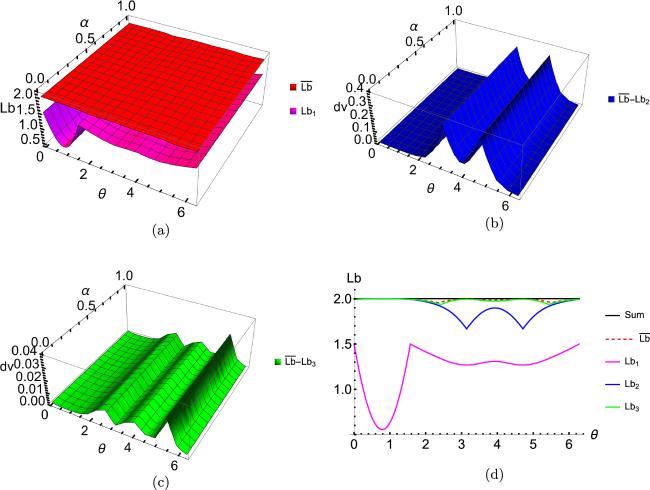
Figure 1. Comparison of the lower bound (Lb) $\overline{{Lb}}$ with Lb1, Lb2 and Lb3. (a) The red surface and the magenta surface represent $\overline{{Lb}}$ and Lb1, respectively. (b) The blue surface represents the difference value (DV) between $\overline{{Lb}}$ and Lb2. (c) The green surface represents the difference value between $\overline{{Lb}}$ and Lb3. (d) For fixed $\alpha =\tfrac{1}{3}$, the black, red dashed, magenta, blue and green curves represent the summation ${{\rm{K}}}_{\rho }^{\tfrac{1}{3}}({\sigma }_{1})+{{\rm{K}}}_{\rho }^{\tfrac{1}{3}}({\sigma }_{2})+{{\rm{K}}}_{\rho }^{\tfrac{1}{3}}({\sigma }_{3})$, $\overline{{Lb}}$, Lb1, Lb2 and Lb3, respectively.

3. Sum uncertainty relations for finite quantum channels

In this section, we give two different types of uncertainty relations associated with arbitrary finite number of quantum channels based on (α, β, γ) MWWYD skew information. We derive an optimal lower bound and show that our bounds are tighter than the existing ones by a detailed example.
Let Φ be a quantum channel with Kraus representation, ${\rm{\Phi }}(\rho )={\sum }_{i=1}^{n}{E}_{i}\rho {E}_{i}^{\dagger }$. In [34] the authors have presented the uncertainty quantification with respect to a channel Φ via (α, β, γ) MWWYD skew information,
$\begin{eqnarray}{{\rm{K}}}_{\rho ,\gamma }^{\alpha ,\beta }({\rm{\Phi }})=\displaystyle \sum _{i=1}^{n}{{\rm{K}}}_{\rho ,\gamma }^{\alpha ,\beta }({E}_{i}),\end{eqnarray}$
where α, β ≥ 0, α + β ≤ 1, 0 ≤ γ ≤ 1. For arbitrary N quantum channels ,Φ1, ⋯ ,ΦN with Kraus representations ${{\rm{\Phi }}}_{t}{(\rho )={\sum }_{i=1}^{n}{E}_{i}^{t}\rho ({E}_{i}^{t})}^{\dagger },\,t\,=\,1,2,\cdots ,N$ (N > 2 for the inequality (22) and N ≥ 2 for the inequalities (2324)). Xu et al. [34] gave the following sum uncertainty quantifications associated with the channels,
$\begin{eqnarray}\begin{array}{rcl}\displaystyle \sum _{t=1}^{N}{{\rm{K}}}_{\rho ,\gamma }^{\alpha ,\beta }({{\rm{\Phi }}}_{t}) & \geqslant & \mathop{\max }\limits_{{\pi }_{t},{\pi }_{s}\in {S}_{n}}\displaystyle \frac{1}{N-2}\\ & & \times \,\left\{\displaystyle \sum _{1\leqslant t\lt s\leqslant N}\displaystyle \sum _{i=1}^{n}{{\rm{K}}}_{\rho ,\gamma }^{\alpha ,\beta }({E}_{{\pi }_{t}(i)}^{t}+{E}_{{\pi }_{s}(i)}^{s})\right.\\ & & \left.-\displaystyle \frac{1}{{\left(N-1\right)}^{2}}\left[\displaystyle \sum _{i=1}^{n}{\left(\displaystyle \sum _{1\leqslant t\lt s\leqslant N}\sqrt{{{\rm{K}}}_{\rho ,\gamma }^{\alpha ,\beta }({E}_{{\pi }_{t}(i)}^{t}+{E}_{{\pi }_{s}(i)}^{s})}\right)}^{2}\right]\right\},\end{array}\end{eqnarray}$
$\begin{eqnarray}\begin{array}{rcl}\displaystyle \sum _{t=1}^{N}{{\rm{K}}}_{\rho ,\gamma }^{\alpha ,\beta }({{\rm{\Phi }}}_{t}) & \geqslant & \mathop{\max }\limits_{{\pi }_{t},{\pi }_{s}\in {S}_{n}}\\ & & \times \,\left\{\displaystyle \frac{1}{N}\displaystyle \sum _{i=1}^{n}{{\rm{K}}}_{\rho ,\gamma }^{\alpha ,\beta }\left(\displaystyle \sum _{t=1}^{N}{E}_{{\pi }_{t}(i)}^{t}\right)\right.\\ & & \left.+\displaystyle \frac{2}{{N}^{2}(N-1)}\left[\displaystyle \sum _{i=1}^{n}{\left(\displaystyle \sum _{1\leqslant t\lt s\leqslant N}\sqrt{{{\rm{K}}}_{\rho ,\gamma }^{\alpha ,\beta }({E}_{{\pi }_{t}(i)}^{t}-{E}_{{\pi }_{s}(i)}^{s})}\right)}^{2}\right]\right\},\end{array}\end{eqnarray}$
$\begin{eqnarray}\begin{array}{rcl}\displaystyle \sum _{t=1}^{N}{{\rm{K}}}_{\rho ,\gamma }^{\alpha ,\beta }({{\rm{\Phi }}}_{t}) & \geqslant & \mathop{\max }\limits_{{\pi }_{t},{\pi }_{s}\in {S}_{n}}\displaystyle \frac{1}{2(N-1)}\\ & & \times \,\left\{\displaystyle \frac{2}{N(N-1)}\left[\displaystyle \sum _{i=1}^{n}{\left(\displaystyle \sum _{1\leqslant t\lt s\leqslant N}\sqrt{{{\rm{K}}}_{\rho ,\gamma }^{\alpha ,\beta }({E}_{{\pi }_{t}(i)}^{t}\pm {E}_{{\pi }_{s}(i)}^{s})}\right)}^{2}\right]\right.\\ & & \left.+\displaystyle \sum _{1\leqslant t\lt s\leqslant N}\displaystyle \sum _{i\,=\,1}^{n}{{\rm{K}}}_{\rho ,\gamma }^{\alpha ,\beta }({E}_{{\pi }_{t}(i)}^{t}\mp {E}_{{\pi }_{s}(i)}^{s})\right\},\end{array}\end{eqnarray}$
where α, β ≥ 0, α + β ≤ 1, 0 ≤ γ ≤ 1, Sn is the n-element permutation group and πt, πsSn are arbitrary n-element permutations. We denote by LB1, LB2 and LB3 the right-hand sides of (22), (23) and (24), respectively.

Let ${{\rm{\Phi }}}_{1},\cdots ,{{\rm{\Phi }}}_{N}$ be N quantum channels with Kraus representations ${{\rm{\Phi }}}_{t}(\rho )={\sum }_{i=1}^{n}{E}_{i}^{t}\rho {\left({E}_{i}^{t}\right)}^{\dagger },\,t\,=\,1,2,\cdots ,N$ ($N\geqslant 2$). We have

$\begin{eqnarray}\displaystyle \sum _{t=1}^{N}{{\rm{K}}}_{\rho ,\gamma }^{\alpha ,\beta }({{\rm{\Phi }}}_{t})\geqslant \max \{{\overline{{LB}}}_{1},{\overline{{LB}}}_{2},{\overline{{LB}}}_{3}\},\end{eqnarray}$
where
$\begin{eqnarray}\begin{array}{rcl}{\overline{{LB}}}_{1} & = & \mathop{\max }\limits_{{\pi }_{t},{\pi }_{s}\in {S}_{n}}\displaystyle \frac{1}{{MN}+(N-2)L}\\ & & \times \,\left\{\displaystyle \frac{2L}{N(N-1)}\left[\displaystyle \sum _{i=1}^{n}{\left(\displaystyle \sum _{1\leqslant t\lt s\leqslant N}\sqrt{{{\rm{K}}}_{\rho ,\gamma }^{\alpha ,\beta }({E}_{{\pi }_{t}(i)}^{t}+{E}_{{\pi }_{s}(i)}^{s})}\right)}^{2}\right]\right.\\ & & \left.+M\displaystyle \sum _{1\leqslant t\lt s\leqslant N}\displaystyle \sum _{i\,=\,1}^{n}{{\rm{K}}}_{\rho ,\gamma }^{\alpha ,\beta }({E}_{{\pi }_{t}(i)}^{t}-{E}_{{\pi }_{s}(i)}^{s})+(M-L)\displaystyle \sum _{i\,=\,1}^{n}{{\rm{K}}}_{\rho ,\gamma }^{\alpha ,\beta }\left(\displaystyle \sum _{t=1}^{N}{E}_{{\pi }_{t}(i)}^{t}\right)\right\},\end{array}\end{eqnarray}$
$\begin{eqnarray}\begin{array}{rcl}{\overline{{LB}}}_{2} & = & \mathop{\max }\limits_{{\pi }_{t},{\pi }_{s}\in {S}_{n}}\displaystyle \frac{1}{{MN}+(N-2)L}\\ & & \times \,\left\{\displaystyle \frac{2M}{N(N-1)}\left[\displaystyle \sum _{i=1}^{n}{\left(\displaystyle \sum _{1\leqslant t\lt s\leqslant N}\sqrt{{{\rm{K}}}_{\rho ,\gamma }^{\alpha ,\beta }({E}_{{\pi }_{t}(i)}^{t}-{E}_{{\pi }_{s}(i)}^{s})}\right)}^{2}\right]\right.\\ & & \left.+L\displaystyle \sum _{1\leqslant t\lt s\leqslant N}\displaystyle \sum _{i\,=\,1}^{n}{{\rm{K}}}_{\rho ,\gamma }^{\alpha ,\beta }({E}_{{\pi }_{t}(i)}^{t}+{E}_{{\pi }_{s}(i)}^{s})+(M-L)\displaystyle \sum _{i\,=\,1}^{n}{{\rm{K}}}_{\rho ,\gamma }^{\alpha ,\beta }\left(\displaystyle \sum _{t=1}^{N}{E}_{{\pi }_{t}(i)}^{t}\right)\right\},\end{array}\end{eqnarray}$
$\begin{eqnarray}\begin{array}{rcl}{\overline{{LB}}}_{3} & = & \mathop{\max }\limits_{{\pi }_{t},{\pi }_{s}\in {S}_{n}}\displaystyle \frac{1}{{MN}+(N-2)L}\\ & & \times \,\left\{\displaystyle \frac{M-L}{{\left(N-1\right)}^{2}}\left[\displaystyle \sum _{i=1}^{n}{\left(\displaystyle \sum _{1\leqslant t\lt s\leqslant N}\sqrt{{{\rm{K}}}_{\rho ,\gamma }^{\alpha ,\beta }({E}_{{\pi }_{t}(i)}^{t}+{E}_{{\pi }_{s}(i)}^{s})}\right)}^{2}\right]\right.\\ & & +L\displaystyle \sum _{1\leqslant t\lt s\leqslant N}\displaystyle \sum _{i=1}^{n}{{\rm{K}}}_{\rho ,\gamma }^{\alpha ,\beta }({E}_{{\pi }_{t}(i)}^{t}+{E}_{{\pi }_{s}(i)}^{s})\\ & & \left.+\,M\displaystyle \sum _{1\leqslant t\lt s\leqslant N}\displaystyle \sum _{i=1}^{n}{{\rm{K}}}_{\rho ,\gamma }^{\alpha ,\beta }({E}_{{\pi }_{t}(i)}^{t}-{E}_{{\pi }_{s}(i)}^{s})\right\},\end{array}\end{eqnarray}$
$\alpha ,\beta \geqslant 0$, $\alpha +\beta \leqslant 1$, $0\leqslant \gamma \leqslant 1$, ${\pi }_{t},{\pi }_{s}\in {S}_{n}$ are arbitrary n-element permutations, the parameters L, M in ${\overline{{LB}}}_{1}$, ${\overline{{LB}}}_{2}$ and ${\overline{{LB}}}_{3}$ satisfy $M\geqslant L\gt 0$, $L\geqslant M\gt 0$ and $L\gt M\gt 0$, respectively.

According to the inequalities (11-13) and equation (7), we have

$\begin{eqnarray*}\begin{array}{rcl}\displaystyle \sum _{t=1}^{N}{{\rm{K}}}_{\rho ,\gamma }^{\alpha ,\beta }({E}_{{\pi }_{t}(i)}^{t}) & \geqslant & \displaystyle \frac{1}{{MN}+(N-2)L}\\ & & \times \,\left\{\displaystyle \frac{2L}{N(N-1)}\left[{\left(\displaystyle \sum _{1\leqslant t\lt s\leqslant N}\sqrt{{{\rm{K}}}_{\rho ,\gamma }^{\alpha ,\beta }({E}_{{\pi }_{t}(i)}^{t}+{E}_{{\pi }_{s}(i)}^{s})}\right)}^{2}\right]\right.\\ & & \left.+M\displaystyle \sum _{1\leqslant t\lt s\leqslant N}{{\rm{K}}}_{\rho ,\gamma }^{\alpha ,\beta }({E}_{{\pi }_{t}(i)}^{t}-{E}_{{\pi }_{s}(i)}^{s})+(M-L){{\rm{K}}}_{\rho ,\gamma }^{\alpha ,\beta }\left(\displaystyle \sum _{t=1}^{N}{E}_{{\pi }_{t}(i)}^{t}\right)\right\},\end{array}\end{eqnarray*}$
for $M\geqslant L\gt 0$,
$\begin{eqnarray*}\begin{array}{rcl}\displaystyle \sum _{t=1}^{N}{{\rm{K}}}_{\rho ,\gamma }^{\alpha ,\beta }({E}_{{\pi }_{t}(i)}^{t}) & \geqslant & \displaystyle \frac{1}{{MN}+(N-2)L}\\ & & \times \,\left\{\displaystyle \frac{2M}{N(N-1)}\left[{\left(\displaystyle \sum _{1\leqslant t\lt s\leqslant N}\sqrt{{{\rm{K}}}_{\rho ,\gamma }^{\alpha ,\beta }({E}_{{\pi }_{t}(i)}^{t}-{E}_{{\pi }_{s}(i)}^{s})}\right)}^{2}\right]\right.\\ & & +L\displaystyle \sum _{1\leqslant t\lt s\leqslant N}{{\rm{K}}}_{\rho ,\gamma }^{\alpha ,\beta }({E}_{{\pi }_{t}(i)}^{t}+{E}_{{\pi }_{s}(i)}^{s})\\ & & \left.+(M-L){{\rm{K}}}_{\rho ,\gamma }^{\alpha ,\beta }\left(\displaystyle \sum _{t=1}^{N}{E}_{{\pi }_{t}(i)}^{t}\right)\right\},\end{array}\end{eqnarray*}$
for $L\geqslant M\gt 0$,
$\begin{eqnarray*}\begin{array}{l}\displaystyle \sum _{t=1}^{N}{{\rm{K}}}_{\rho ,\gamma }^{\alpha ,\beta }({E}_{{\pi }_{t}(i)}^{t})\geqslant \displaystyle \frac{1}{{MN}+(N-2)L}\\ \,\times \,\left\{\displaystyle \frac{M-L}{{\left(N-1\right)}^{2}}\left[{\left(\displaystyle \sum _{1\leqslant t\lt s\leqslant N}\sqrt{{{\rm{K}}}_{\rho ,\gamma }^{\alpha ,\beta }({E}_{{\pi }_{t}(i)}^{t}+{E}_{{\pi }_{s}(i)}^{s})}\right)}^{2}\right]\right.\\ \,\left.+L\displaystyle \sum _{1\leqslant t\lt s\leqslant N}{{\rm{K}}}_{\rho ,\gamma }^{\alpha ,\beta }({E}_{{\pi }_{t}(i)}^{t}+{E}_{{\pi }_{s}(i)}^{s})\right.\\ \,\left.+M\displaystyle \sum _{1\leqslant t\lt s\leqslant N}{{\rm{K}}}_{\rho ,\gamma }^{\alpha ,\beta }({E}_{{\pi }_{t}(i)}^{t}-{E}_{{\pi }_{s}(i)}^{s})\right\},\end{array}\end{eqnarray*}$
for $L\gt M\gt 0$. Summing over the index i, which implies theorem 2.

Let ${{\rm{\Phi }}}_{1},\cdots ,{{\rm{\Phi }}}_{N}$ be N quantum channels with Kraus representations ${{\rm{\Phi }}}_{t}{(\rho )={\sum }_{i=1}^{n}{E}_{i}^{t}\rho ({E}_{i}^{t})}^{\dagger },\,t\,=\,1,2,\cdots ,N$ ($N\geqslant 2$), we have the sum uncertainty relations with respect to WWYD skew information,

$\begin{eqnarray}\begin{array}{rcl}\displaystyle \sum _{t=1}^{N}{{\rm{K}}}_{\rho }^{\alpha }({{\rm{\Phi }}}_{t}) & \geqslant & \mathop{\max }\limits_{{\pi }_{t},{\pi }_{s}\in {S}_{n}}\displaystyle \frac{1}{{MN}+(N-2)L}\\ & & \times \,\left\{\displaystyle \frac{2L}{N(N-1)}\left[\displaystyle \sum _{i=1}^{n}{\left(\displaystyle \sum _{1\leqslant t\lt s\leqslant N}\sqrt{{{\rm{K}}}_{\rho }^{\alpha }({E}_{{\pi }_{t}(i)}^{t}+{E}_{{\pi }_{s}(i)}^{s})}\right)}^{2}\right]\right.\\ & & +M\displaystyle \sum _{1\leqslant t\lt s\leqslant N}\displaystyle \sum _{i\,=\,1}^{n}{{\rm{K}}}_{\rho }^{\alpha }({E}_{{\pi }_{t}(i)}^{t}-{E}_{{\pi }_{s}(i)}^{s})\\ & & \left.+(M-L)\displaystyle \sum _{i\,=\,1}^{n}{{\rm{K}}}_{\rho }^{\alpha }\left(\displaystyle \sum _{t=1}^{N}{E}_{{\pi }_{t}(i)}^{t}\right)\right\},\end{array}\end{eqnarray}$
$\begin{eqnarray}\begin{array}{rcl}\displaystyle \sum _{t=1}^{N}{{\rm{K}}}_{\rho }^{\alpha }({{\rm{\Phi }}}_{t}) & \geqslant & \mathop{\max }\limits_{{\pi }_{t},{\pi }_{s}\in {S}_{n}}\displaystyle \frac{1}{{MN}+(N-2)L}\\ & & \times \,\left\{\displaystyle \frac{2M}{N(N-1)}\left[\displaystyle \sum _{i=1}^{n}{\left(\displaystyle \sum _{1\leqslant t\lt s\leqslant N}\sqrt{{{\rm{K}}}_{\rho }^{\alpha }({E}_{{\pi }_{t}(i)}^{t}-{E}_{{\pi }_{s}(i)}^{s})}\right)}^{2}\right]\right.\\ & & +L\displaystyle \sum _{1\leqslant t\lt s\leqslant N}\displaystyle \sum _{i\,=\,1}^{n}{{\rm{K}}}_{\rho }^{\alpha }({E}_{{\pi }_{t}(i)}^{t}+{E}_{{\pi }_{s}(i)}^{s})\\ & & \left.+(M-L)\displaystyle \sum _{i\,=\,1}^{n}{{\rm{K}}}_{\rho }^{\alpha }\left(\displaystyle \sum _{t=1}^{N}{E}_{{\pi }_{t}(i)}^{t}\right)\right\},\end{array}\end{eqnarray}$
$\begin{eqnarray}\begin{array}{rcl}\displaystyle \sum _{t=1}^{N}{{\rm{K}}}_{\rho }^{\alpha }({{\rm{\Phi }}}_{t}) & \geqslant & \mathop{\max }\limits_{{\pi }_{t},{\pi }_{s}\in {S}_{n}}\displaystyle \frac{1}{{MN}+(N-2)L}\\ & & \times \,\left\{\displaystyle \frac{M-L}{{\left(N-1\right)}^{2}}\left[\displaystyle \sum _{i=1}^{n}{\left(\displaystyle \sum _{1\leqslant t\lt s\leqslant N}\sqrt{{{\rm{K}}}_{\rho }^{\alpha }({E}_{{\pi }_{t}(i)}^{t}+{E}_{{\pi }_{s}(i)}^{s})}\right)}^{2}\right]\right.\\ & & +L\displaystyle \sum _{1\leqslant t\lt s\leqslant N}\displaystyle \sum _{i\,=\,1}^{n}{{\rm{K}}}_{\rho }^{\alpha }({E}_{{\pi }_{t}(i)}^{t}+{E}_{{\pi }_{s}(i)}^{s})\\ & & \left.+M\displaystyle \sum _{1\leqslant t\lt s\leqslant N}\displaystyle \sum _{i\,=\,1}^{n}{{\rm{K}}}_{\rho }^{\alpha }({E}_{{\pi }_{t}(i)}^{t}-{E}_{{\pi }_{s}(i)}^{s})\right\},\end{array}\end{eqnarray}$
where $0\leqslant \alpha \leqslant 1$, the parameters L, M in (29), (30) and (31) satisfy $M\geqslant L\gt 0$, $L\geqslant M\gt 0$ and $L\gt M\gt 0$, respectively.

Thus we have ${\sum }_{i=1}^{N}{{\rm{K}}}_{\rho }^{\alpha }({{\rm{\Phi }}}_{t})\geqslant \max \{{rhs}29,{rhs}30,{rhs}31\}$, where rhs29, rhs30 and rhs31 represent the right-hand sides of inequalities (29), (30) and (31), respectively.
The uncertainty quantification of quantum channel Φ based on (α, β, γ) MWWYD skew information can also be written as [35],
$\begin{eqnarray}{{\rm{K}}}_{\rho ,\gamma }^{\alpha ,\beta }({\rm{\Phi }})=\displaystyle \frac{1}{2}\mathrm{Tr}({u}^{\dagger }u)=\displaystyle \frac{1}{2}\parallel u{\parallel }^{2},\end{eqnarray}$
where α, β ≥ 0, α + β ≤ 1, 0 ≤ γ ≤ 1, $u=(\left[(1-\gamma ){\rho }^{\alpha }+\gamma {\rho }^{\beta },{E}_{1}\right]{\rho }^{\tfrac{1-\alpha -\beta }{2}}$, $\left[(1-\gamma ){\rho }^{\alpha }+\gamma {\rho }^{\beta },{E}_{2}\right] \times {\rho }^{\tfrac{1-\alpha -\beta }{2}}$, $\cdots$ ,$\left[(1-\gamma ){\rho }^{\alpha }+\gamma {\rho }^{\beta },{E}_{n}\right]{\rho }^{\tfrac{1-\alpha -\beta }{2}})$. Therefore, on the basis of $\parallel {u}_{t}\pm {u}_{s}{\parallel }^{2}=2{\sum }_{i=1}^{n}{{\rm{K}}}_{\rho ,\gamma }^{\alpha ,\beta }({E}_{i}^{t}\pm {E}_{i}^{s})$, $\parallel {u}_{t}{\parallel }^{2}\,=2{{\rm{K}}}_{\rho ,\gamma }^{\alpha ,\beta }({{\rm{\Phi }}}_{t})$ and the inequalities (1113), we have the following theorem.

Let ${{\rm{\Phi }}}_{1},\cdots ,{{\rm{\Phi }}}_{N}$ be N quantum channels with Kraus representations ${{\rm{\Phi }}}_{t}(\rho )={\sum }_{i=1}^{n}{E}_{i}^{t}\rho {\left({E}_{i}^{t}\right)}^{\dagger },\,t=1,2,\cdots ,N$ ($N\geqslant 2$). We have

$\begin{eqnarray}\displaystyle \sum _{t=1}^{N}{{\rm{K}}}_{\rho ,\gamma }^{\alpha ,\beta }({{\rm{\Phi }}}_{t})\geqslant \max \{\overline{{LB}}1,\overline{{LB}}2,\overline{{LB}}3\},\end{eqnarray}$
where
$\begin{eqnarray}\begin{array}{rcl}\overline{{LB}}1 & = & \mathop{\max }\limits_{{\pi }_{t},{\pi }_{s}\in {S}_{n}}\displaystyle \frac{1}{{MN}+(N-2)L}\\ & & \times \,\left\{\displaystyle \frac{2L}{N(N-1)}{\left[\displaystyle \sum _{1\leqslant t\lt s\leqslant N}\sqrt{\displaystyle \sum _{i=1}^{n}{{\rm{K}}}_{\rho ,\gamma }^{\alpha ,\beta }({E}_{{\pi }_{t}(i)}^{t}+{E}_{{\pi }_{s}(i)}^{s})}\right]}^{2}\right.\\ & & +M\displaystyle \sum _{1\leqslant t\lt s\leqslant N}\displaystyle \sum _{i\,=\,1}^{n}{{\rm{K}}}_{\rho ,\gamma }^{\alpha ,\beta }({E}_{{\pi }_{t}(i)}^{t}-{E}_{{\pi }_{s}(i)}^{s})\\ & & \left.+(M-L)\displaystyle \sum _{i\,=\,1}^{n}{{\rm{K}}}_{\rho ,\gamma }^{\alpha ,\beta }\left(\displaystyle \sum _{t=1}^{N}{E}_{{\pi }_{t}(i)}^{t}\right)\right\},\end{array}\end{eqnarray}$
$\begin{eqnarray}\begin{array}{rcl}\overline{{LB}}2 & = & \mathop{\max }\limits_{{\pi }_{t},{\pi }_{s}\in {S}_{n}}\displaystyle \frac{1}{{MN}+(N-2)L}\\ & & \times \,\left\{\displaystyle \frac{2M}{N(N-1)}{\left[\displaystyle \sum _{1\leqslant t\lt s\leqslant N}\sqrt{\displaystyle \sum _{i=1}^{n}{{\rm{K}}}_{\rho ,\gamma }^{\alpha ,\beta }({E}_{{\pi }_{t}(i)}^{t}-{E}_{{\pi }_{s}(i)}^{s})}\right]}^{2}\right.\\ & & +L\displaystyle \sum _{1\leqslant t\lt s\leqslant N}\displaystyle \sum _{i=1}^{n}{{\rm{K}}}_{\rho ,\gamma }^{\alpha ,\beta }({E}_{{\pi }_{t}(i)}^{t}+{E}_{{\pi }_{s}(i)}^{s})\\ & & \left.+(M-L)\displaystyle \sum _{i=1}^{n}{{\rm{K}}}_{\rho ,\gamma }^{\alpha ,\beta }\left(\displaystyle \sum _{t=1}^{N}{E}_{{\pi }_{t}(i)}^{t}\right)\right\},\end{array}\end{eqnarray}$
$\begin{eqnarray}\begin{array}{rcl}\overline{{LB}}3 & = & \mathop{\max }\limits_{{\pi }_{t},{\pi }_{s}\in {S}_{n}}\displaystyle \frac{1}{{MN}+(N-2)L}\\ & & \times \,\left\{\displaystyle \frac{M-L}{{\left(N-1\right)}^{2}}{\left[\displaystyle \sum _{1\leqslant t\lt s\leqslant N}\sqrt{\displaystyle \sum _{i=1}^{n}{{\rm{K}}}_{\rho ,\gamma }^{\alpha ,\beta }({E}_{{\pi }_{t}(i)}^{t}+{E}_{{\pi }_{s}(i)}^{s})}\right]}^{2}\right.\\ & & +L\displaystyle \sum _{1\leqslant t\lt s\leqslant N}\displaystyle \sum _{i=1}^{n}{{\rm{K}}}_{\rho ,\gamma }^{\alpha ,\beta }({E}_{{\pi }_{t}(i)}^{t}+{E}_{{\pi }_{s}(i)}^{s})\\ & & \left.+M\displaystyle \sum _{1\leqslant t\lt s\leqslant N}\displaystyle \sum _{i=1}^{n}{{\rm{K}}}_{\rho ,\gamma }^{\alpha ,\beta }({E}_{{\pi }_{t}(i)}^{t}-{E}_{{\pi }_{s}(i)}^{s})\right\},\end{array}\end{eqnarray}$
$\alpha ,\beta \geqslant 0$, $\alpha +\beta \leqslant 1$, $0\leqslant \gamma \leqslant 1$, ${\pi }_{t},{\pi }_{s}\in {S}_{n}$ are arbitrary n-element permutations, and the parameters L, M in $\overline{{LB}}1$, $\overline{{LB}}2$ and $\overline{{LB}}3$ satisfy $M\geqslant L\gt 0$, $L\geqslant M\gt 0$ and $L\gt M\,\gt 0$, respectively.

According to appendix C in [45], it is not hard to prove that our lower bound $\max \{\overline{{LB}}1,\overline{{LB}}2,\overline{{LB}}3\}$ is tighter than the lower bound ${LB}=\max \{{LB}1,{LB}2,{LB}3\}$ given in [35].
Motivated by the results given in appendix D of [45], we have an optimal lower bound,
$\begin{eqnarray}\displaystyle \sum _{t=1}^{N}{{\rm{K}}}_{\rho ,\gamma }^{\alpha ,\beta }({{\rm{\Phi }}}_{t})\geqslant \max \{\overline{{LB}}1,\overline{{LB}}2,{\overline{{LB}}}_{3}\},\end{eqnarray}$
where ${\overline{{LB}}}_{3}$ is given in theorem 2. For convenience we denote by $\overline{{LB}}$ on the right-hand side of (37), $\overline{{LB}}=\max \{\overline{{LB}}1,\overline{{LB}}2,{\overline{{LB}}}_{3}\}$.
To illustrate our results, we consider the MWWYD skew information as a special case, and take M = 2, L = 1 for $\overline{{LB}}1$, and M = 1, L = 2 for $\overline{{LB}}2$ and ${\overline{{LB}}}_{3}$.

Consider the mixed state given by the Bloch vector ${\boldsymbol{r}}=(\tfrac{\sqrt{2}}{2}\cos \theta ,\tfrac{\sqrt{2}}{2}\sin \theta ,0)$, $\rho =\tfrac{1}{2}({{\rm{I}}}_{2}+{\boldsymbol{r}}\cdot {\boldsymbol{\sigma }})$, where $0\leqslant \theta \leqslant \pi $, ${{\rm{I}}}_{2}$ is the 2 × 2 identity matrix and ${\boldsymbol{\sigma }}=({\sigma }_{1},{\sigma }_{2},{\sigma }_{3})$ is given by the Pauli matrices. We consider the following three quantum channels:

i

(i)the phase damping channel ${{\rm{\Phi }}}_{{\rm{PD}}}$,

$\begin{eqnarray*}\begin{array}{l}{{\rm{\Phi }}}_{{\rm{PD}}}(\rho )=\displaystyle \sum _{i=1}^{2}{A}_{i}\rho {A}_{i}^{\dagger },\quad {A}_{1}=| 0\rangle \langle 0| +\sqrt{1-q}| 1\rangle \langle 1| ,\\ {A}_{2}=\sqrt{q}| 1\rangle \langle 1| ;\end{array}\end{eqnarray*}$

ii

(ii)the amplitude damping channel ${{\rm{\Phi }}}_{{\rm{AD}}}$,

$\begin{eqnarray*}\begin{array}{l}{{\rm{\Phi }}}_{{\rm{AD}}}(\rho )=\displaystyle \sum _{i=1}^{2}{B}_{i}\rho {B}_{i}^{\dagger },\quad {B}_{1}=| 0\rangle \langle 0| +\sqrt{1-q}| 1\rangle \langle 1| ,\\ {B}_{2}=\sqrt{q}| 0\rangle \langle 1| ;\end{array}\end{eqnarray*}$

iii

(iii)the bit flip channel ${{\rm{\Phi }}}_{{\rm{BF}}}$,

$\begin{eqnarray*}\begin{array}{l}{{\rm{\Phi }}}_{{\rm{BF}}}(\rho )=\displaystyle \sum _{i=1}^{2}{C}_{i}\rho {C}_{i}^{\dagger },\quad {C}_{1}=\sqrt{q}(| 0\rangle \langle 0| +| 1\rangle \langle 1| ),\\ {C}_{2}=\sqrt{1-q}(| 0\rangle \langle 1| +| 1\rangle \langle 0| ),\end{array}\end{eqnarray*}$
with $0\leqslant q\lt 1$. We compare the lower bounds $\overline{{LB}}$, LB, LB3, LB2, LB1 with the sum $={{\rm{K}}}_{\rho }^{\tfrac{1}{4}}({{\rm{\Phi }}}_{{\rm{AD}}})+{{\rm{K}}}_{\rho }^{\tfrac{1}{4}}({{\rm{\Phi }}}_{{\rm{PD}}})\,+{{\rm{K}}}_{\rho }^{\tfrac{1}{4}}({{\rm{\Phi }}}_{{\rm{BF}}})$ for $\alpha =\tfrac{1}{4}$, q = 0.3. It is shown that our new lower bound $\overline{{LB}}$ is tighter than LB, LB3, LB2 and LB1, see figure 2.

Figure 2. (a) The solid black, solid red and solid blue curves represent the sum $=\,{{\rm{K}}}_{\rho }^{\tfrac{1}{4}}({{\rm{\Phi }}}_{{AD}})+{{\rm{K}}}_{\rho }^{\tfrac{1}{4}}({{\rm{\Phi }}}_{{PD}})+{{\rm{K}}}_{\rho }^{\tfrac{1}{4}}({{\rm{\Phi }}}_{{BF}})$ , the lower bounds (Lb) $\overline{{LB}}$ and LB, respectively. The dashed green, dashed blue and dashed magenta curves represent the lower bounds LB3, LB2 and LB1, respectively. (b-d) The solid green curve denotes the difference value (DV) between $\overline{{LB}}$ and LB, LB3 and LB2, respectively.

4. Sum uncertainty relations for finite unitary channels

In [35] we introduced the (α, β, γ) MWWYD skew information of a unitary operator U,
$\begin{eqnarray}\begin{array}{rcl}{{\rm{K}}}_{\rho ,\gamma }^{\alpha ,\beta }(U) & = & -\displaystyle \frac{1}{2}\mathrm{Tr}([(1-\gamma ){\rho }^{\alpha }+\gamma {\rho }^{\beta },{U}^{\dagger }][(1-\gamma ){\rho }^{\alpha }+\gamma {\rho }^{\beta },U]{\rho }^{1-\alpha -\beta })\\ & = & \displaystyle \frac{1}{2}{\parallel \left[(1-\gamma ){\rho }^{\alpha }+\gamma {\rho }^{\beta },U\right]{\rho }^{\displaystyle \frac{1-\alpha -\beta }{2}}\parallel }^{2},\\ & & \alpha ,\beta \geqslant 0,\,\alpha +\beta \leqslant 1,\,0\leqslant \gamma \leqslant 1.\end{array}\end{eqnarray}$
Associated with a unitary channel ΦU(ρ) = UρU, we denote ${{\rm{K}}}_{\rho ,\gamma }^{\alpha ,\beta }(U)$ the related quantity of the unitary channel ΦU. By employing $\parallel \left({\sum }_{t=1}^{N}{u}_{t}\right){\parallel }^{2}\,=\,2{{\rm{K}}}_{\rho ,\gamma }^{\alpha ,\beta }\left({\sum }_{t=1}^{N}{U}_{t}\right)$, $\parallel {u}_{t}{\parallel }^{2}=2{{\rm{K}}}_{\rho ,\gamma }^{\alpha ,\beta }({U}_{t})$, $\parallel {u}_{t}\pm {u}_{s}{\parallel }^{2}=2{{\rm{K}}}_{\rho ,\gamma }^{\alpha ,\beta }({U}_{t}\pm {U}_{s})$ and the inequalities (1113) , we have the following theorem.

Let ${U}_{1},\cdots ,{U}_{N}$ be N unitary operators, we have

$\begin{eqnarray}\displaystyle \sum _{t=1}^{N}{{\rm{K}}}_{\rho ,\gamma }^{\alpha ,\beta }({U}_{t})\geqslant \max \{\overline{{Lb}}1,\overline{{Lb}}2,\overline{{Lb}}3\},\end{eqnarray}$
where
$\begin{eqnarray}\begin{array}{rcl}\overline{{Lb}}1 & = & \displaystyle \frac{1}{{MN}+(N-2)L}\\ & & \times \,\left\{\displaystyle \frac{2L}{N(N-1)}{\left[\displaystyle \sum _{1\leqslant t\lt s\leqslant N}\sqrt{{{\rm{K}}}_{\rho ,\gamma }^{\alpha ,\beta }({U}_{t}+{U}_{s})}\right]}^{2}\right.\\ & & +M\displaystyle \sum _{1\leqslant t\lt s\leqslant N}{{\rm{K}}}_{\rho ,\gamma }^{\alpha ,\beta }({U}_{t}-{U}_{s})+(M-L){{\rm{K}}}_{\rho ,\gamma }^{\alpha ,\beta }\\ & & \left.\times \,\left(\displaystyle \sum _{t=1}^{N}{U}_{t}\right)\right\},\end{array}\end{eqnarray}$
with $M\geqslant L\gt 0$,
$\begin{eqnarray}\begin{array}{rcl}\overline{{Lb}}2 & = & \displaystyle \frac{1}{{MN}+(N-2)L}\\ & & \times \,\left\{\displaystyle \frac{2M}{N(N-1)}{\left[\displaystyle \sum _{1\leqslant t\lt s\leqslant N}\sqrt{{{\rm{K}}}_{\rho ,\gamma }^{\alpha ,\beta }({U}_{t}-{U}_{s})}\right]}^{2}\right.\\ & & +L\displaystyle \sum _{1\leqslant t\lt s\leqslant N}{{\rm{K}}}_{\rho ,\gamma }^{\alpha ,\beta }({U}_{t}+{U}_{s})\\ & & \left.+(M-L){{\rm{K}}}_{\rho ,\gamma }^{\alpha ,\beta }\left(\displaystyle \sum _{t=1}^{N}{U}_{t}\right)\right\},\end{array}\end{eqnarray}$
with $L\geqslant M\gt 0$,
$\begin{eqnarray}\begin{array}{rcl}\overline{{Lb}}3 & = & \displaystyle \frac{1}{{MN}+(N-2)L}\\ & & \times \,\left\{\displaystyle \frac{M-L}{{\left(N-1\right)}^{2}}{\left[\displaystyle \sum _{1\leqslant t\lt s\leqslant N}\sqrt{{{\rm{K}}}_{\rho ,\gamma }^{\alpha ,\beta }({U}_{t}+{U}_{s})}\right]}^{2}\right.\\ & & +L\displaystyle \sum _{1\leqslant t\lt s\leqslant N}{{\rm{K}}}_{\rho ,\gamma }^{\alpha ,\beta }({U}_{t}+{U}_{s})\\ & & \left.+M\displaystyle \sum _{1\leqslant t\lt s\leqslant N}{{\rm{K}}}_{\rho ,\gamma }^{\alpha ,\beta }({U}_{t}-{U}_{s})\right\},\end{array}\end{eqnarray}$
with $L\gt M\gt 0$, $\alpha ,\beta \geqslant 0$, $\alpha +\beta \leqslant 1$ and $0\leqslant \gamma \leqslant 1$.

For convenience we denote by $\widetilde{{Lb}}$ on the right-hand side of (39), $\widetilde{{Lb}}=\max \{\overline{{Lb}}1,\overline{{Lb}}2,\overline{{Lb}}3\}$ and compare the lower bound with ${Lb}=\max \{{Lb}1,{Lb}2,{Lb}3\}$ in [35]. In the example below we consider the MWWYD skew information with M = 2, L = 1 for $\overline{{Lb}}1$, and M = 1, L = 2 for $\overline{{Lb}}2$ and $\overline{{Lb}}3$.

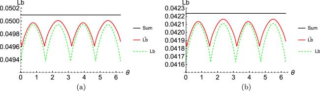
Suppose that $\rho =\tfrac{1}{2}({{\rm{I}}}_{2}+{\boldsymbol{r}}\cdot {\boldsymbol{\sigma }})$ with ${\boldsymbol{r}}\,=(\tfrac{\sqrt{3}}{3}\cos \theta ,\tfrac{\sqrt{3}}{3}\sin \theta ,0)$. Consider the following three unitary operators generated by Pauli matrices,

$\begin{eqnarray*}\begin{array}{l}{U}_{1}={{\rm{e}}}^{\tfrac{{\rm{i}}\pi {\sigma }_{1}}{8}}=\left(\begin{array}{c}\cos \displaystyle \frac{\pi }{8}\ \mathrm{isin}\displaystyle \frac{\pi }{8}\\ \mathrm{isin}\displaystyle \frac{\pi }{8}\ \cos \displaystyle \frac{\pi }{8}\end{array}\right),\\ {U}_{2}={{\rm{e}}}^{\tfrac{{\rm{i}}\pi {\sigma }_{2}}{8}}=\left(\begin{array}{c}\cos \displaystyle \frac{\pi }{8}\ \sin \displaystyle \frac{\pi }{8}\\ -\sin \displaystyle \frac{\pi }{8}\ \cos \displaystyle \frac{\pi }{8}\end{array}\right),\\ {U}_{3}={{\rm{e}}}^{\tfrac{{\rm{i}}\pi {\sigma }_{3}}{8}}=\left(\begin{array}{c}{e}^{{\rm{i}}\displaystyle \frac{\pi }{8}}\quad 0\\ \ 0\ {e}^{-{\rm{i}}\displaystyle \frac{\pi }{8}}\end{array}\right),\end{array}\end{eqnarray*}$
which correspond to the Bloch sphere rotations of $-\tfrac{\pi }{4}$ around the x axis, the y axis and z axis, respectively. We compare the lower bounds $\widetilde{{Lb}}$, Lb with the sum $=\,{{\rm{K}}}_{\rho }^{\alpha }({{\rm{\Phi }}}_{{\rm{AD}}})+{{\rm{K}}}_{\rho }^{\alpha }({{\rm{\Phi }}}_{{\rm{PD}}})+{{\rm{K}}}_{\rho }^{\alpha }({{\rm{\Phi }}}_{{\rm{BF}}})$ via MWWYD skew information for $\alpha =\tfrac{1}{3}$ and $\alpha =\tfrac{1}{5}$, respectively. Our new lower bound $\widetilde{{Lb}}$ is tighter than Lb, see figure 3.

Figure 3. The solid black, red and green dashed curves represent the sum $=\,{{\rm{K}}}_{\rho }^{\alpha }({U}_{1})+{{\rm{K}}}_{\rho }^{\alpha }({U}_{2})+{{\rm{K}}}_{\rho }^{\alpha }({U}_{3})$, $\widetilde{{Lb}}$ and Lb, respectively. (a) $\alpha =\tfrac{1}{3};$ (b) $\alpha =\tfrac{1}{5}$.

5. Conclusions

We have presented tighter uncertainty relations via (α, β, γ) WWYD skew information for multiple observables, quantum channels and unitary channels. By explicit examples, we have shown that our uncertainty inequalities are tighter than the existing results given in [34, 35]. Our results are also valid for the WY, WWYD and (α, γ) WWYD skew information as the special cases. Uncertainty relations give rise to fundamental limitations on quantum physical quantities, and our results may shed new light on the understanding of uncertainty relations and their applications in quantum information processing such as communication security.

Conflict of interest

The authors declare that they have no conflict of interest.

This work was supported by National Natural Science Foundation of China (Grant Nos. 12161056, 12075159, 12171044); Jiangxi Provincial Natural Science Foundation (Grant No. 20232ACB211003); and the Academician Innovation Platform of Hainan Province.

1
Heisenberg W 1927 Über den anschaulichen Inhalt der quantentheoretischen Kinematik und Mechanik Z Phys. 43 172

DOI

2
Robertson H P 1929 The uncertainty principle Phys. Rev. 34 163

DOI

3
Deutsch D 1983 Uncertainty in quantum measurements Phys. Rev. Lett. 50 631

DOI

4
Maassen H Uffink J B M 1988 Generalized entropic uncertainty relations Phys. Rev. Lett. 60 1103

DOI

5
Wehner S Winter A 2010 Entropic uncertainty relations-a survey New J. Phys. 12 025009

DOI

6
Wu S Yu S Mølmer K 2009 Entropic uncertainty relation for mutually unbiased bases Phys. Rev. A 79 022104

DOI

7
Rastegin A E 2013 Uncertainty relations for MUBs and SIC-POVMs in terms of generalized entropies Eur. Phys. J. D 67 269

DOI

8
Gudder S 2007 Operator probability theory Int. J. Pure Appl. Math. 39 511

9
Dou Y Du H 2013 Generalizations of the Heisenberg and Schrödinger uncertainty relations J. Math. Phys. 54 103508

DOI

10
Dou Y Du H 2014 Note on the Wigner-Yanase-Dyson skew information Int. J. Theor. Phys. 53 952

DOI

11
Sun Y Li N 2021 The uncertainty of quantum channels in terms of variance Quantum Inf. Process. 20 25

DOI

12
Srinivas M D 2003 Optimal entropic uncertainty relation for successive measurements in quantum information theory Pramana J. Phys. 60 1137

DOI

13
Rudnicki Ł Puchała Z Zyczkowski K 2014 Strong majorization entropic uncertainty relations Phys. Rev. A 89 052115

DOI

14
Puchała Z Rudnicki Ł Zyczkowski K 2013 Majorization entropic uncertainty relations J. Phys. A: Math. Theor. 46 272002

DOI

15
Rudnicki Ł 2015 Majorization approach to entropic uncertainty relations for coarse-grained observables Phys. Rev. A 91 032123

DOI

16
Friedland S Gheorghiu V Gour G 2013 Universal uncertainty relations Phys. Rev. Lett. 111 230401

DOI

17
Wigner E P Yanase M M 1963 Information contents of distributions Proc. Natl. Acad. Sci. 49 910-918

DOI

18
Chen P Luo S 2007 Direct approach to quantum extensions of Fisher information Front. Math. 2 359

DOI

19
Wu Z Zhang L Fei S-M Li-Jost X 2020 Coherence and complementarity based on modified generalized skew information Quantum Inf. Process. 19 154

DOI

20
Wu Z Zhang L Wang J Li-Jost X Fei S-M 2020 Uncertainty relations based on modified Wigner-Yanase-Dyson skew information Int. J. Theor. Phys. 59 704

DOI

21
Luo S 2003 Wigner-Yanase skew information and uncertainty relations Phys. Rev. Lett. 91 180403

DOI

22
Luo S Zhang Q 2004 On skew information IEEE Trans. Inf. Theory 50 1778

DOI

23
Cai L Luo S 2008 On convexity of generalized Wigner-Yanase-Dyson information Lett. Math. Phys. 83 253

DOI

24
Yanagi K 2010 Uncertainty relation on Wigner-Yanase-Dyson skew information J. Math. Anal. Appl. 365 12

DOI

25
Yanagi K 2010 Wigner-Yanase-Dyson skew information and uncertainty relation J. Phys. Conf. Ser. 201 012015

26
Xu C Wu Z Fei S-M 2022 Uncertainty of quantum channels via modified generalized variance and modified generalized Wigner-Yanase-Dyson skew information Quantum Inf. Process. 21 292

DOI

27
Wu Z Zhang L Fei S-M Wang J 2022 Skew information-based coherence generating power of quantum channels Quantum Inf. Process. 21 236

DOI

28
Wu Z Zhang L Fei S-M Li-Jost X 2021 Average skew information-based coherence and its typicality for random quantum states J. Phys. A: Math. Theor. 54 015302

DOI

29
Wu Z Huang H Fei S-M Li-Jost X 2020 Geometry of skew information-based quantum coherence Commun. Theor. Phys. 72 105102

DOI

30
Huang H Wu Z Fei S-M 2020 Uncertainty and complementarity relations based on generalized skew information Europhys. Lett. 132 60007

DOI

31
Furuichi S Yanagi K Kuriyama K 2009 Trace inequalities on a generalized Wigner-Yanase skew information J. Math. Anal. Appl. 356 179

DOI

32
Chen Z Liang L Li H Wang W 2016 Two generalized Wigner-Yanase skew information and their uncertainty relations Quantum Inf. Process. 15 5107

DOI

33
Zhang Z 2021 Trace inequalities based on two-parameter extended Wigner-Yanase skew information J. Math. Anal. Appl. 497 124851

DOI

34
Xu C Wu Z Fei S-M 2022 Sum uncertainty relations based on (α, β γ) weighted Wigner-Yanase-Dyson skew information Int. J. Theor. Phys. 61 185

DOI

35
Xu C Wu Z Fei S-M 2022 Tighter uncertainty relations based on (α, β γ) modified weighted Wigner-Yanase-Dyson skew information of quantum channels Laser Phys. Lett. 19 105206

DOI

36
Nielson M A Chuang I L 2010 Quanutm Computation and Quantum Information Cambridge Cambridge University Press

37
Busch P Grabowski M Lahti P 1997 Operational Quantum Physics Berlin Springer 2nd ed.

38
Chen B Fei S-M Long G-L 2016 Sum uncertainty relations based on Wigner-Yanase skew information Quantum Inf. Process. 15 2639

DOI

39
Fu S Sun Y Luo S 2019 Skew information-based uncertainty relations for quantum channels Quantum Inf. Process. 18 258

DOI

40
Zhang L Gao T Yan F 2021 Tighter uncertainty relations based on Wigner-Yanase skew information for observables and channels Phys. Lett. A 387 127029

DOI

41
Zhang Q Wu J Fei S-M 2021 A note on uncertainty relations of arbitrary N quantum channels Laser Phys. Lett. 18 095204

DOI

42
Cai L 2021 Sum uncertainty relations based on metric-adjusted skew information Quantum Inf. Process. 20 72

DOI

43
Zhang Q Wu J Ma X Fei S-M 2023 A note on uncertainty relations of metric-adjusted skew information Quantum Inf. Process. 22 115

DOI

44
Ren R Li P Ye M Li Y 2021 Tighter sum uncertainty relations based on metric-adjusted skew information Phys. Rev. A 104 052414

DOI

45
Li H Gao T Yan F 2023 Tighter sum uncertainty relations via metric-adjusted skew information Phys. Scr. 98 015024

DOI

Outlines

/