


1. Introduction
Plasma, an electrically conducting quasi-neutral gas comprising charged particles that collectively move, also contains molecules and photons across various wavelengths. Plasma constitutes a major portion of the observable universe. Its charged particle motion facilitates the propagation of electromagnetic waves. The magnetosphere surrounding the Earth contains dense, cold plasma, causing electromagnetic waves interacting with the Earth's atmosphere to naturally serve as a source for radio communication. This specific type of plasma, found within the Earth's magnetosphere, is categorized as non-thermal due to the significantly higher temperature of electrons compared to ions and neutrals [1]. The non-thermal nature of cold plasma holds particular significance in biomedicine. It exhibits the capability to eliminate cancer cells and activate specific signaling pathways that are crucial in treatment responses, offering a novel and innovative approach to combat cancer [2]. Plasma-filled waveguides find application in converting methane into hydrogen or synthesis gas, essential for producing raw chemicals like methanol and ammonia, as well as functioning as hydrogenation agents in oil refineries and reducing gases in the steel industry [3].
Wait [4] explained that in the presence of a constant magnetic field, the dielectric constant of a plasma is in the form of a tensor. He gave explicit results for the reflection coefficients of stratified plasma in planar and cylindrical geometry.
Waveguides are structures that direct the propagation of energy in a channel. The variation of geometric settings and material properties has a significant impact on the scattering characteristics of the channel. Analytical mode-matching methods are found to be useful for analysis of the energy propagation in a waveguide. The technique has recently been advanced in various directions to investigate the scattering behavior of acoustic waves at structural discontinuities: for instance, see [5-10]. The transfer of electromagnetic energy using plasma waveguides has always been an interest of researchers [11-15]. A study of plasma waveguides shows that their properties differ, in many significant aspects, from those of conventional dielectric waveguides.
The scattering of microwaves propagating through a circular waveguide, partially filled with a homogeneous lossless and cold electron plasma, was studied by Gehre et al [16]. After finding the plasma dielectric tensor analytically, investigations were performed by Khalil and Mousa of the electromagnetic wave propagation in a plasma-filled cylindrical waveguide [17]. Dvorak et al [18] investigated the propagation of an ultra-wide-band electromagnetic pulse in a homogeneous cold plasma, and the reflection and absorption of a polarized wave in an inhomogeneous disspative magnetized plasma slab were investigated analytically by Jazi et al [19]. The solution to the scattering of plane electromagnetic waves by an anisotropic sphere with plasma was obtained by Geng et al [20]. A multiscale property in a Janus metastructure can be achieved by adjusting the incident angle of electromagnetic waves, by arranging the dielectrics asymmetrically, and by using the anisotropy of the plasma [21, 22]. The scattering of microwaves from a plasma column in a rectangular waveguide has also been discussed [23, 24].
To analyze the scattering of electromagnetic waves in cold plasma-filled waveguides, different numerical techniques have been applied [25-35]. The mode-matching technique is often applicable in solving discontinuity problems in isotropic waveguides [36]. This technique has been applied to write a high-frequency structure to analyze the program for the resonator of gyro-devices [37]. The electromagnetic wave transmission from a lossless isotropic cylindrical waveguide with metallic walls to a semi-bounded plasma, using the mode-matching technique, has also been analyzed [38]. Rao et al [39] observed that the total phase retarder bandwidth can reach 2.6 GHz by appropriately optimizing the incident angle, the plasma frequency, the external magnetic field and the nonlinear light intensity.
It is noted that the investigations conducted in most of the above-mentioned papers are restricted to cylindrical waveguides or circular columns in rectangular waveguides. With a few exceptions, the electromagnetic propagation in rectangular waveguides has not been widely discussed. Therefore, the originality of this work is the analysis of electromagnetic wave scattering in a parallel-plate waveguide, with a groove, containing a slab of cold unmagnetized plasma. To the best of our knowledge, this kind of attempt has not been made in the past. The solution of the problem has a significant purpose as waveguides are an integral part of resonators and plasma propulsion engines. This article provides a rigorous study of electromagnetic scattering in a two-dimensional parallel-plate rectangular waveguide, which contains a slab of cold plasma bounded by metallic strips, placed in a groove in the central region. The same physical configuration is discussed for a plasma slab placed, without strips, between layers of a dielectric.
The semi-analytic technique of mode matching is used to investigate electromagnetic wave scattering at discontinuities in the considered waveguide. It is a fast and convergent method, which can be applied easily without any discretization of variables. This technique provides an exact solution to electromagnetic scattering problems in both discontinuous and planar structures. In this work, the mode-matching method provides the solution for different parameters, frequencies and dimensions of heights of the cold plasma and dielectric media.
The article is arranged as follows: section 2 states the physical aspects of the problem and gives a brief description of the topic. In section 3 , the eigenfunctions of the formulated boundary value problem are obtained by the governing Helmholtz equation and boundary conditions. The system thus obtained is solved numerically to calculate the transmission and reflection coefficients. The energy identity is proved in section 4 . In section 5 , simulations are performed for both frequency regimes, i.e. the transparency regime (the electromagnetic wave frequency is higher than the plasma frequency) and the non-transparency regime (the electromagnetic wave frequency is lower than the plasma frequency). Power analysis is also carried out for varying heights in both frequency regimes. The coefficients of reflection and transmission are also obtained with reference to the normalized wave frequency for transparency and non-transparency regions. Section 6 presents the summary and conclusions drawn for the two frequency regimes in dielectric and plasma regions.
2. Formulation of propagating waves within a plasma slab
The analysis of electromagnetic wave scattering discussed in this article is centered around a plasma slab, which is either enclosed between perfect electric conductor (PEC) plates or embedded within a dielectric medium. The physical configuration depicted in figure 1 represents the arrangement of the central region of the metallic waveguide in which the scattering is analyzed. An H-polarized incident wave is considered to be propagating in the positive x direction within this setting. This incident wave is assumed to be the fundamental duct mode, with unit amplitude, propagating from the left inlet to interfaces on the right. The incident angle is presumed to be making a zero angle with the x-axis. Copper or silver can be used as plates in this waveguide. In figure 1(a), the plasma slab is bounded by PEC walls, whereas in figure 1(b), the plasma slab is encompassed by a dielectric medium. The dimensions of the plasma slab adhere to the conditions ∣y∣ < a and ∣x∣ < L, while the PEC walls in figure 1(a) are positioned at y = ± a, ± b, and in figure 1(b), the PEC walls are located at y = ± b. The region between ∣y∣ > a and ∣y∣ < b is considered to be a dielectric medium with permittivity ε0 and permeability μ0. This configuration corresponds to a wave number k0, which is defined as ${k}_{0}=\omega \sqrt{{\mu }_{0}{\epsilon }_{0}}$, where ω represents the angular frequency and c denotes the speed of light, expressed as $c=\sqrt{1/{\epsilon }_{0}{\mu }_{0}}$. This relation implies that k0 can be expressed as k0 = ω/c. However, for a cold plasma, the permeability remains μ0, and the permittivity tensor $\overline{\epsilon }$, as specified in [40] and [41], is
$\begin{eqnarray*}\overline{\epsilon }=\left[\begin{array}{ccc}{\epsilon }_{1} & -{\rm{i}}{\epsilon }_{2} & 0\\ {\rm{i}}{\epsilon }_{2} & {\epsilon }_{1} & 0\\ 0 & 0 & {\epsilon }_{3}\end{array}\right],\end{eqnarray*}$
where ${\epsilon }_{1}=1-\displaystyle \frac{{\omega }_{{\rm{p}}}^{2}}{{\omega }^{2}-{\omega }_{{\rm{c}}}^{2}},\,{\epsilon }_{2}=\displaystyle \frac{{\omega }_{{\rm{c}}}{\omega }_{{\rm{p}}}^{2}}{\omega \left({\omega }^{2}-{\omega }_{{\rm{c}}}^{2}\right)}$ and ${\epsilon }_{3}\,=1-\displaystyle \frac{{\omega }_{{\rm{p}}}^{2}}{{\omega }^{2}}$. Here, the quantities ωp and ωc stand for the frequencies associated with plasma and cyclotron effects, respectively. The exponential temporal variation e−iωt is considered and consistently omitted [42].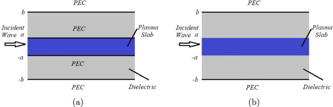
Figure 1. The cold plasma slab configuration: (a) enclosed by metal strips, and (b) embedded within a dielectric environment. |
Maxwell's equations dictate the propagation of electromagnetic waves in a waveguide. Faraday's law, presented below, remains valid for both dielectric and cold plasma mediums:
$\begin{eqnarray}{\rm{\nabla }}\times {\boldsymbol{E}}={\rm{i}}\omega {\boldsymbol{B}}.\end{eqnarray}$
The expression of Ampere's law within the context of dielectrics is as follows: $\begin{eqnarray}{\rm{\nabla }}\times {\boldsymbol{B}}=-{\rm{i}}\displaystyle \frac{\omega }{{c}^{2}}{\boldsymbol{E}},\end{eqnarray}$
while in a cold plasma, this law is formulated as: $\begin{eqnarray}{\rm{\nabla }}\times {\boldsymbol{B}}=-\displaystyle \frac{{\rm{i}}}{\omega }{k}_{0}^{2}\overline{\epsilon }.{\boldsymbol{E}}.\end{eqnarray}$
For a two-dimensional waveguide (∂/∂z = 0), the electromagnetic fields E and B include longitudinal components Ez and Bz and transverse components Ex, Ey, Bx and By. For electromagnetic wave propagation, the Maxwell's equations are solved together with boundary and interface conditions. In a dielectric, the longitudinal components satisfy the Helmholtz equation $\begin{eqnarray}\left(\displaystyle \frac{{\partial }^{2}}{\partial {x}^{2}}+\displaystyle \frac{{\partial }^{2}}{\partial {y}^{2}}+{k}_{0}^{2}\right)\left(\begin{array}{c}{E}_{z}\\ {B}_{z}\end{array}\right)=\left(\begin{array}{c}0\\ 0\end{array}\right),\end{eqnarray}$
whereas the transverse components can be found using the information from the longitudinal components, as given below: $\begin{eqnarray*}{E}_{x}=-\displaystyle \frac{{c}^{2}}{{\rm{i}}\omega }\displaystyle \frac{\partial {B}_{z}}{\partial y},\quad {E}_{y}=\displaystyle \frac{{c}^{2}}{i\omega }\displaystyle \frac{\partial {B}_{z}}{\partial x},\end{eqnarray*}$
$\begin{eqnarray*}{B}_{x}=\displaystyle \frac{1}{i\omega }\displaystyle \frac{\partial {E}_{z}}{\partial y},\quad {B}_{y}=-\displaystyle \frac{1}{i\omega }\displaystyle \frac{\partial {E}_{z}}{\partial x}.\end{eqnarray*}$
For cold unmagnetized plasma, the Helmholtz equation is expressed, in longitudinal components of fields, as [43] $\begin{eqnarray}\left(\displaystyle \frac{{\partial }^{2}}{\partial {x}^{2}}+\displaystyle \frac{{\partial }^{2}}{\partial {y}^{2}}+{k}_{1}^{2}\right)\left(\begin{array}{c}{E}_{z}\\ {B}_{z}\end{array}\right)=\left(\begin{array}{c}0\\ 0\end{array}\right).\end{eqnarray}$
The transverse components can be given as $\begin{eqnarray*}{E}_{x}=\displaystyle \frac{{\rm{i}}\omega }{{k}_{1}^{2}}\displaystyle \frac{\partial {B}_{z}}{\partial y},\quad {E}_{y}=-\displaystyle \frac{i\omega }{{k}_{1}^{2}}\displaystyle \frac{\partial {B}_{z}}{\partial x},\end{eqnarray*}$
$\begin{eqnarray*}{B}_{x}=\displaystyle \frac{1}{i\omega }\displaystyle \frac{\partial {E}_{z}}{\partial y},\quad {B}_{y}=-\displaystyle \frac{1}{i\omega }\displaystyle \frac{\partial {E}_{z}}{\partial x}.\end{eqnarray*}$
The wave number of cold plasma medium is indicated as ${k}_{1}=\displaystyle \frac{\omega }{c}\sqrt{1-\displaystyle \frac{{\omega }_{{\rm{p}}}^{2}}{{\omega }^{2}}}$, where ωp is the plasma frequency.In the presence of a magnetic field, like the case of upper atmosphere, the cyclotron frequency ωc is nonzero. All the components of the permittivity tensor $\overline{\epsilon }$ are present, which significantly affect the Helmholtz equation and transverse components of the electric field. Hence, the matching conditions are transformed. To determine the wave propagation in the regions presented in figure 1, equations (4 ) and (5 ) are solved subject to boundary and interface conditions. For an H-polarized setting, the traveling wave formulation is explained in the next subsection.
2.1. Plasma slab enclosed by metal strips
For plasma in metallic strips, the PEC boundary conditions at the walls y = ±a and ±b are as 5 ), subject to equation (6 ) with the separation of the variable technique, the eigenfunction expansion formation can be achieved as:
$\begin{eqnarray}\displaystyle \frac{\partial {B}_{z}}{\partial y}(x,\pm a)=0=\displaystyle \frac{\partial {B}_{z}}{\partial y}(x,\pm b).\end{eqnarray}$
Upon solving equation ( $\begin{eqnarray}{B}_{z}(x,y)=\left\{\begin{array}{l}\displaystyle \sum _{n=0}^{\infty }\left({B}_{n}^{(1)}{{\rm{e}}}^{{\rm{i}}{\zeta }_{n}x}+{C}_{n}^{(1)}{{\rm{e}}}^{-{\rm{i}}{\zeta }_{n}x}\right){Y}_{1n}(y),\\ \displaystyle \sum _{n=0}^{\infty }\left({B}_{n}^{(2)}{{\rm{e}}}^{{\rm{i}}{\lambda }_{n}x}+{C}_{n}^{(2)}{{\rm{e}}}^{-{\rm{i}}{\lambda }_{n}x}\right){Y}_{2n}(y),\\ \displaystyle \sum _{n=0}^{\infty }\left({B}_{n}^{(3)}{{\rm{e}}}^{{\rm{i}}{\zeta }_{n}x}+{C}_{n}^{(3)}{{\rm{e}}}^{-{\rm{i}}{\zeta }_{n}x}\right){Y}_{3n}(y),\end{array}\right.\end{eqnarray}$
where ${B}_{n}^{(j)}$ and ${C}_{n}^{(j)},\,j\,=\,1,2,3$ exhibit the amplitudes in the respective regions −b < y < − a, a < y < a and a < y < b. The wave numbers of nth modes in these regions are ${\zeta }_{n}=\sqrt{{k}_{0}^{2}-{\left(\displaystyle \frac{n\pi }{b-a}\right)}^{2}}$ and ${\lambda }_{n}=\sqrt{{k}_{1}^{2}-{\left(\displaystyle \frac{n\pi }{2a}\right)}^{2}},$ n = 0, 1, 2, … Here, the eigenfunctions ${Y}_{1n}(y)=\cos \left\{\Space{0ex}{1.75em}{0ex}\left(\displaystyle \frac{n\pi }{b-a}\right)(y+b)\right\}$, ${Y}_{2n}(y)=\cos \left\{\Space{0ex}{1.59em}{0ex}\left(\displaystyle \frac{n\pi }{2a}\right)(y+a)\right\}$ and ${Y}_{3n}(y)=\cos \left\{\Space{0ex}{1.65em}{0ex}\left(\displaystyle \frac{n\pi }{b-a}\right)(y-b)\right\}$ are orthogonal and satisfy the usual orthogonality relations, $\begin{eqnarray}\left.\begin{array}{r}{\displaystyle \int }_{-b}^{-a}{Y}_{1m}{Y}_{1n}{\rm{d}}{y}={\delta }_{{mn}}\left(\displaystyle \frac{b-a}{2}\right){\epsilon }_{m},\\ {\displaystyle \int }_{-a}^{a}{Y}_{2m}{Y}_{2n}{\rm{d}}{y}={\delta }_{{mn}}a{\epsilon }_{m},\\ {\displaystyle \int }_{a}^{b}{Y}_{3m}{Y}_{3n}{\rm{d}}{y}={\delta }_{{mn}}\left(\displaystyle \frac{b-a}{2}\right){\epsilon }_{m},\end{array}\right\}\end{eqnarray}$
where δmn is the Kronecker delta and εm = 2 for m = 0 and 1 otherwise.2.2. Plasma slab embedded within a dielectric environment
For a slab embedded within a dielectric environment, the interface and PEC boundary conditions are as follows 5 ) subject to equations (10 )-(14 ) with the separation of the variable technique, the eigenfunction expansion formation can be achieved as
$\begin{eqnarray}{B}_{z}(x,-{a}^{-})={B}_{z}(x,-{a}^{+}),\,\end{eqnarray}$
$\begin{eqnarray}{B}_{z}(x,{a}^{-})={B}_{z}(x,{a}^{+}),\end{eqnarray}$
$\begin{eqnarray}{\eta }_{0}\displaystyle \frac{\partial {B}_{z}}{\partial y}(x,-{a}^{-})={\eta }_{1}\displaystyle \frac{\partial {B}_{z}}{\partial y}(x,-{a}^{+}),\,\end{eqnarray}$
$\begin{eqnarray}{\eta }_{1}\displaystyle \frac{\partial {B}_{z}}{\partial y}(x,{a}^{-})={\eta }_{0}\displaystyle \frac{\partial {B}_{z}}{\partial y}(x,{a}^{+}),\,\end{eqnarray}$
$\begin{eqnarray}\displaystyle \frac{\partial {B}_{z}}{\partial y}(x,\pm b)=0,\,\end{eqnarray}$
where the respective surface impedances of dielectric and cold plasma, η0 and η1, are related to wave numbers in these mediums as ${\eta }_{0}=1/{k}_{0}^{2}$ and ${\eta }_{1}=1/{k}_{1}^{2}$. Upon solving equation ( $\begin{eqnarray}{B}_{z}(x,y)=\displaystyle \sum _{n=0}^{\infty }({B}_{n}{{\rm{e}}}^{{{\rm{i}}{s}}_{n}x}+{C}_{n}{{\rm{e}}}^{-{{\rm{i}}{s}}_{n}x}){Y}_{n}(y),\end{eqnarray}$
where Bn and Cn represent the amplitudes of the nth mode. The eigenfunction Yn(y) in the groove can be manifested as, $\begin{eqnarray}{Y}_{n}(y)=\left\{\begin{array}{ll}{Y}_{1n}(y), & -b\lt y\lt -a,\\ {Y}_{2n}(y), & -a\lt y\lt a,\\ {Y}_{3n}(y), & a\lt y\lt b,\end{array}\right.\end{eqnarray}$
where $\begin{eqnarray}{Y}_{1n}(y)=\cosh [{\tau }_{n}(y+b)],\end{eqnarray}$
$\begin{eqnarray}\begin{array}{l}{Y}_{2n}(y)=\displaystyle \frac{1}{{\eta }_{1}{\gamma }_{n}}\\ \quad \quad \times \left\{{\eta }_{0}{\tau }_{n}\sinh [{\tau }_{n}(b-a)]\sinh [{\gamma }_{n}(y+a)]\right\}\\ \quad \quad +\,\cosh [{\tau }_{n}(b-a)]\cosh [{\gamma }_{n}(y+a)],\end{array}\end{eqnarray}$
$\begin{eqnarray}\begin{array}{l}{Y}_{3n}(y)=\displaystyle \frac{\cosh [{\tau }_{n}(y-b)]}{{\eta }_{1}{\gamma }_{n}\cosh [{\tau }_{n}(b-a)]}\left\{{\eta }_{0}{\tau }_{n}\right.\\ \quad \times \,\left.\sinh [{\tau }_{n}(b-a)]\sinh (2{\gamma }_{n}a)\right\}\\ \quad +\,{\eta }_{1}{\gamma }_{n}\cosh [{\tau }_{n}(y-b)]\cosh (2{\gamma }_{n}a),\end{array}\end{eqnarray}$
satisfy the orthogonality relation as given below $\begin{eqnarray}\begin{array}{l}{\eta }_{0}{\displaystyle \int }_{-b}^{-a}{Y}_{1m}{Y}_{1n}{\rm{d}}{y}+{\eta }_{1}{\displaystyle \int }_{-a}^{a}{Y}_{2m}{Y}_{2n}{\rm{d}}{y}\\ \quad +\,{\eta }_{0}{\displaystyle \int }_{a}^{b}{Y}_{3m}{Y}_{3n}{\rm{d}}{y}={\delta }_{{mn}}{E}_{m},\end{array}\end{eqnarray}$
where $\begin{eqnarray}\begin{array}{l}{E}_{n}={\eta }_{0}{\displaystyle \int }_{-b}^{-a}{Y}_{1n}^{2}{\rm{d}}{y}+{\eta }_{1}\\ \quad \times \,{\displaystyle \int }_{-a}^{a}{Y}_{2n}^{2}{\rm{d}}{y}+{\eta }_{0}{\displaystyle \int }_{a}^{b}{Y}_{3n}^{2}{\rm{d}}{y}.\end{array}\end{eqnarray}$
The quantities τn and γn, written as ${\tau }_{n}=\sqrt{{s}_{n}^{2}-{k}_{0}^{2}}$ and ${\gamma }_{n}=\sqrt{{s}_{n}^{2}-{k}_{1}^{2}}$, represent the roots of the characteristic equation, $\begin{eqnarray}\begin{array}{l}{\eta }_{0}^{2}{\tau }_{n}^{2}{\sinh }^{2}[{\tau }_{n}(b-a)]\sinh (2{\gamma }_{n}a)+{\eta }_{1}^{2}{\gamma }_{n}^{2}\\ \quad \quad \times \,{\cosh }^{2}[{\tau }_{n}(b-a)]\sinh (2{\gamma }_{n}a)\\ \quad \quad +\,{\eta }_{0}{\eta }_{1}{\tau }_{n}{\gamma }_{n}\sinh [2{\tau }_{n}(b-a)]\cosh (2{\gamma }_{n}a)=0.\end{array}\end{eqnarray}$
Here, sn indicates the wave number of the nth mode inside the groove.3. Scattering from plasma slab: a mode-matching formulation
Within this context, the plasma slabs discussed in the preceding section are applied within the central segment (∣x∣ < L) of the waveguide that extends infinitely along the x-axis. The physical arrangement of both cases is depicted in figure 2. The study involves the analysis of the scattering of electromagnetic waves by the plasma slab, by considering their initiation from the region at x < -L and their subsequent interaction with the plasma-contained region as they exit the domain at x > L.
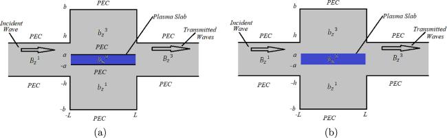
Figure 2. The waveguide configuration: (a) enclosed by metal strips, and (b) embedded within a dielectric environment. |
We contemplate an incident H-polarized wave, propagating within this partially confined waveguide, in the positive x direction. The complete magnetic field, denoted by the field potential ${B}_{z}^{(T)}(x,y)$, is expressed as follows:
$\begin{eqnarray}{B}_{z}^{(T)}(x,y)=\left\{\begin{array}{ll}{B}_{z}^{(1)}(x,y), & x\lt -L,\quad -h\lt y\lt h,\\ {B}_{z}^{(2)}(x,y), & | x| \lt L,\quad -b\lt y\lt b,\\ {B}_{z}^{(3)}(x,y), & x\gt L,\quad -h\lt y\lt h.\end{array}\right.\end{eqnarray}$
Utilizing the mode-matching technique involves establishing the eigenfunction expansions and corresponding orthogonality criteria within each distinct region of the waveguide.By employing a variable separable approach, the scattered fields within the regions x < − L and x > L can be demonstrated to take on the following representation:
$\begin{eqnarray}\begin{array}{l}{B}_{z}^{(1)}(x,y)={{\rm{e}}}^{{{\rm{i}}{k}}_{0}(x+L)}+\displaystyle \sum _{n=0}^{\infty }{A}_{n}{{\rm{e}}}^{-i{\nu }_{n}(x+L)}{\phi }_{n}(y),\\ \,-h\lt y\lt h,\end{array}\end{eqnarray}$
$\begin{eqnarray}\begin{array}{l}{B}_{z}^{(3)}(x,y)=\displaystyle \sum _{n=0}^{\infty }{D}_{n}{{\rm{e}}}^{{\rm{i}}{\nu }_{n}(x-L)}{\phi }_{n}(y),\\ \,-h\lt y\lt h.\end{array}\end{eqnarray}$
Here, νn, with n taking values of 0, 1, 2, and so forth, represents the wave number of the nth mode within the regions x < − L and x > L. The amplitudes An and Dn define the strengths of these modes, while the eigenfunctions φn(y) can be expressed as, $\begin{eqnarray*}{\phi }_{n}(y)=\cosh \left[\displaystyle \frac{n\pi }{2h}(y+h)\right].\end{eqnarray*}$
These fields satisfy the Helmholtz equation and boundary conditions on perfectly conducting walls.The eigenexpansion of ${B}_{z}^{(2)}$ can be extracted from equations (7 ) and (14 ) for the plasma slab enclosed by metallic strips and for the slab embedded in a dielectric environment, respectively.
It is worthwhile to note that the amplitudes appearing in the eigenexpansions (7 ), (14 ), (23 ) and (24 ) are unknowns and can be determined by implementing the matching conditions at the two interfaces.
3.1. Matching conditions
The continuity of fields at the interfaces x = -L and x = L infers the following matching conditions,
$\begin{eqnarray}{B}_{z}^{(p)}(\pm L,y)={B}_{z}^{(2)}(\pm L,y),\,-h\leqslant y\leqslant h,\end{eqnarray}$
$\begin{eqnarray}\displaystyle \frac{\partial {B}_{z}^{(2)}}{\partial x}(\pm L,y)=\left\{\begin{array}{ll}0, & -b\leqslant y\leqslant -h,\\ \displaystyle \frac{\partial {B}_{z}^{(p)}}{\partial x}(\pm L,y), & -h\leqslant y\leqslant -a,\end{array}\right.\end{eqnarray}$
$\begin{eqnarray}\displaystyle \frac{\partial {B}_{z}^{(2)}}{\partial x}(\pm L,y)=\displaystyle \frac{{\eta }_{0}}{{\eta }_{1}}\displaystyle \frac{\partial {B}_{z}^{(p)}}{\partial x}(\pm L,y),\,-a\leqslant y\leqslant a,\end{eqnarray}$
$\begin{eqnarray}\displaystyle \frac{\partial {B}_{z}^{(2)}}{\partial x}(\pm L,y)=\left\{\begin{array}{ll}\displaystyle \frac{\partial {B}_{z}^{(p)}}{\partial x}(\pm L,y), & a\leqslant y\leqslant h,\\ 0, & h\leqslant y\leqslant b,\end{array}\right.\end{eqnarray}$
where p = 1 for the field at interface x = − L and p = 3 at interface x = L.3.2. Plasma slab enclosed by metal strips
Employing the matching conditions, equation (25 ), together with some mathematical rearrangements leads to 29 ) and (30 ) leads to 30 ) from equation (29 ) submits
$\begin{eqnarray}\begin{array}{l}{A}_{m}=-{\delta }_{m0}+\displaystyle \frac{1}{{\epsilon }_{m}h}\displaystyle \sum _{n=0}^{\infty }\left({B}_{n}^{(1)}{{\rm{e}}}^{-{\rm{i}}{\zeta }_{n}L}+{C}_{n}^{(1)}{{\rm{e}}}^{{\rm{i}}{\zeta }_{n}L}\right){P}_{{mn}}\\ \,+\,\displaystyle \frac{1}{{\epsilon }_{m}h}\displaystyle \sum _{n=0}^{\infty }\left({B}_{n}^{(2)}{{\rm{e}}}^{-{\rm{i}}{\lambda }_{n}L}+{C}_{n}^{(2)}{{\rm{e}}}^{{\rm{i}}{\lambda }_{n}L}\right){Q}_{{mn}}\\ \,+\,\displaystyle \frac{1}{{\epsilon }_{m}h}\displaystyle \sum _{n=0}^{\infty }\left({B}_{n}^{(3)}{{\rm{e}}}^{-{\rm{i}}{\zeta }_{n}L}+{C}_{n}^{(3)}{{\rm{e}}}^{{\rm{i}}{\zeta }_{n}L}\right){R}_{{mn}},\end{array}\end{eqnarray}$
$\begin{eqnarray}\begin{array}{l}{D}_{m}=\displaystyle \frac{1}{{\epsilon }_{m}h}\displaystyle \sum _{n=0}^{\infty }\left({B}_{n}^{(1)}{{\rm{e}}}^{{\rm{i}}{\zeta }_{n}L}+{C}_{n}^{(1)}{{\rm{e}}}^{-{\rm{i}}{\zeta }_{n}L}\right){P}_{{mn}}\\ \,+\,\displaystyle \frac{1}{{\epsilon }_{m}h}\displaystyle \sum _{n=0}^{\infty }\left({B}_{n}^{(2)}{{\rm{e}}}^{{\rm{i}}{\lambda }_{n}L}+{C}_{n}^{(2)}{{\rm{e}}}^{-{\rm{i}}{\lambda }_{n}L}\right){Q}_{{mn}}\\ \,+\,\displaystyle \frac{1}{{\epsilon }_{m}h}\displaystyle \sum _{n=0}^{\infty }\left({B}_{n}^{(3)}{{\rm{e}}}^{{\rm{i}}{\zeta }_{n}L}+{C}_{n}^{(3)}{{\rm{e}}}^{-{\rm{i}}{\zeta }_{n}L}\right){R}_{{mn}},\end{array}\end{eqnarray}$
where $\begin{eqnarray*}\begin{array}{l}{P}_{{mn}}={\displaystyle \int }_{-h}^{-a}{\phi }_{m}(y){Y}_{1n}(y){\rm{d}}{y},\\ {Q}_{{mn}}=\,{\displaystyle \int }_{-a}^{a}{\phi }_{m}(y){Y}_{2n}(y){\rm{d}}{y},\\ {R}_{{mn}}=\,{\displaystyle \int }_{a}^{h}{\phi }_{m}(y){Y}_{3n}(y){\rm{d}}{y}.\end{array}\end{eqnarray*}$
Adding equations ( $\begin{eqnarray}\begin{array}{l}{{\rm{\Psi }}}_{m}^{+}=-{\delta }_{m0}+\displaystyle \frac{2}{h{\epsilon }_{m}}\left\{\displaystyle \sum _{n=0}^{\infty }{{\rm{\Phi }}}_{1n}^{+}\cos ({\zeta }_{n}L){P}_{{mn}}\right.\\ \quad \left.+\,{{\rm{\Phi }}}_{2n}^{+}\cos ({\lambda }_{n}L){Q}_{{mn}}+{{\rm{\Phi }}}_{3n}^{+}\cos ({\zeta }_{n}L){R}_{{mn}}\right\},\end{array}\end{eqnarray}$
while subtracting equation ( $\begin{eqnarray}\begin{array}{l}{{\rm{\Psi }}}_{m}^{-}=-{\delta }_{m0}-\displaystyle \frac{2{\rm{i}}}{h{\epsilon }_{m}}\left\{\displaystyle \sum _{n=0}^{\infty }{{\rm{\Phi }}}_{1n}^{-}\sin ({\zeta }_{n}L){P}_{{mn}}\right.\\ \quad \left.+\,{{\rm{\Phi }}}_{2n}^{-}\sin ({\lambda }_{n}L){Q}_{{mn}}+{{\rm{\Phi }}}_{3n}^{-}\sin ({\zeta }_{n}L){R}_{{mn}}\right\},\end{array}\end{eqnarray}$
where ${{\rm{\Psi }}}_{m}^{\pm }={A}_{m}\pm {D}_{m}$ and ${{\rm{\Phi }}}_{{jm}}^{\pm }={B}_{m}^{(j)}\pm {C}_{m}^{(j)},j\,=\,1,2,3.$Deploying the conditions of equation (26 ) to equation (28 ) at the interface x = L capitulates 26 ) to (28 ) in the same above-mentioned manner, displays 33 ) from (36 ), (34 ) from (37 ) and (35 ) from (38 ) leads to the formation of the following equations 33 ) and (36 ), (35 ) and (37 ), and (36 ) and (38 ) forms ${{\rm{\Phi }}}_{1m}^{-},{{\rm{\Phi }}}_{2m}^{-}$ and ${{\rm{\Phi }}}_{3m}^{-}$ in the following way 31 ), (32 ) and (39 )-(44 ) reveal a system of infinite equations that have the unknowns $\left\{{A}_{n},{B}_{n}^{(j)},{C}_{n}^{(j)},{D}_{n}\right\},\,j\,=1,2,3.$ The system is truncated and is solved numerically, and the results will be explored in the numerical discussion section.
$\begin{eqnarray}\begin{array}{l}\left({B}_{m}^{(1)}{{\rm{e}}}^{-{\rm{i}}{\zeta }_{m}L}-{C}_{m}^{(1)}{{\rm{e}}}^{{\rm{i}}{\zeta }_{m}L}\right)=\displaystyle \frac{2}{{\zeta }_{m}{\epsilon }_{m}(b-a)}\\ \quad \quad \times \,\left\{{k}_{0}{P}_{0m}-\displaystyle \sum _{n=0}^{\infty }{A}_{n}{\nu }_{n}{P}_{{nm}}\right\},\end{array}\end{eqnarray}$
$\begin{eqnarray}\begin{array}{l}\left({B}_{m}^{(2)}{{\rm{e}}}^{-{\rm{i}}{\lambda }_{m}L}-{C}_{m}^{(2)}{{\rm{e}}}^{{\rm{i}}{\lambda }_{m}L}\right)=\displaystyle \frac{{\eta }_{0}}{{\eta }_{1}{\lambda }_{m}{\epsilon }_{m}a}\\ \quad \quad \times \,\left\{{k}_{0}{Q}_{0m}-\displaystyle \sum _{n=0}^{\infty }{A}_{n}{\nu }_{n}{Q}_{{nm}}\right\},\end{array}\end{eqnarray}$
$\begin{eqnarray}\begin{array}{l}\left({B}_{m}^{(3)}{{\rm{e}}}^{-{\rm{i}}{\zeta }_{m}L}-{C}_{m}^{(3)}{{\rm{e}}}^{{\rm{i}}{\zeta }_{m}L}\right)=\displaystyle \frac{2}{{\zeta }_{m}{\epsilon }_{m}(b-a)}\\ \quad \quad \times \,\left\{{k}_{0}{R}_{0m}-\displaystyle \sum _{n=0}^{\infty }{A}_{n}{\nu }_{n}{R}_{{nm}}\right\}.\end{array}\end{eqnarray}$
Again, employing the matching conditions of equations ( $\begin{eqnarray}\begin{array}{l}\left({B}_{m}^{(1)}{{\rm{e}}}^{{\rm{i}}{\zeta }_{m}L}-{C}_{m}^{(1)}{{\rm{e}}}^{-{\rm{i}}{\zeta }_{m}L}\right)\\ \quad =\,\displaystyle \frac{2}{{\zeta }_{m}{\epsilon }_{m}(b-a)}\displaystyle \sum _{n=0}^{\infty }{D}_{n}{\nu }_{n}{P}_{{nm}},\end{array}\end{eqnarray}$
$\begin{eqnarray}\begin{array}{l}\left({B}_{m}^{(2)}{{\rm{e}}}^{{\rm{i}}{\lambda }_{m}L}-{C}_{m}^{(2)}{{\rm{e}}}^{-{\rm{i}}{\lambda }_{m}L}\right)\\ \quad =\,\displaystyle \frac{{\eta }_{0}}{{\eta }_{1}{\lambda }_{m}{\epsilon }_{m}a}\displaystyle \sum _{n=0}^{\infty }{D}_{n}{\nu }_{n}{Q}_{{nm}},\end{array}\end{eqnarray}$
$\begin{eqnarray}\begin{array}{l}\left({B}_{m}^{(3)}{{\rm{e}}}^{{\rm{i}}{\zeta }_{m}L}-{C}_{m}^{(3)}{{\rm{e}}}^{-{\rm{i}}{\zeta }_{m}L}\right)\\ \quad =\,\displaystyle \frac{2}{{\zeta }_{m}{\epsilon }_{m}(b-a)}\displaystyle \sum _{n=0}^{\infty }{D}_{n}{\nu }_{n}{R}_{{nm}}.\end{array}\end{eqnarray}$
Subtracting equations ( $\begin{eqnarray}\begin{array}{l}{{\rm{\Phi }}}_{1m}^{+}=\displaystyle \frac{{\rm{i}}}{{\zeta }_{m}{\epsilon }_{m}\sin ({\zeta }_{m}L)(b-a)}\\ \quad \times \,\left({k}_{0}{P}_{0m}-\displaystyle \sum _{n=0}^{\infty }{{\rm{\Psi }}}_{n}^{+}{\nu }_{n}{P}_{{nm}}\right),\end{array}\end{eqnarray}$
$\begin{eqnarray}\begin{array}{l}{{\rm{\Phi }}}_{2m}^{+}=\displaystyle \frac{{\rm{i}}{\eta }_{0}}{2{\eta }_{1}{\lambda }_{m}{\epsilon }_{m}a\sin ({\lambda }_{m}L)}\\ \quad \times \,\left({k}_{0}{Q}_{0m}-\displaystyle \sum _{n=0}^{\infty }{{\rm{\Psi }}}_{n}^{+}{\nu }_{n}{Q}_{{nm}}\right),\end{array}\end{eqnarray}$
$\begin{eqnarray}\begin{array}{l}{{\rm{\Phi }}}_{3m}^{+}=\displaystyle \frac{{\rm{i}}}{{\zeta }_{m}{\epsilon }_{m}\sin ({\zeta }_{m}L)(b-a)}\\ \quad \times \,\left({k}_{0}{R}_{0m}-\displaystyle \sum _{n=0}^{\infty }{{\rm{\Psi }}}_{n}^{+}{\nu }_{n}{R}_{{nm}}\right).\end{array}\end{eqnarray}$
Now, respective adding of equations ( $\begin{eqnarray}\begin{array}{l}{{\rm{\Phi }}}_{1m}^{-}=\displaystyle \frac{1}{{\zeta }_{m}{\epsilon }_{m}\cos ({\zeta }_{m}L)(b-a)}\\ \quad \times \,\left({k}_{0}{P}_{0m}-\displaystyle \sum _{n=0}^{\infty }{{\rm{\Psi }}}_{n}^{-}{\nu }_{n}{P}_{{nm}}\right),\end{array}\end{eqnarray}$
$\begin{eqnarray}\begin{array}{l}{{\rm{\Phi }}}_{2m}^{-}=\displaystyle \frac{{\eta }_{0}}{2{\eta }_{1}{\lambda }_{m}{\epsilon }_{m}a\cos ({\lambda }_{m}L)}\\ \quad \times \,\left({k}_{0}{Q}_{0m}-\displaystyle \sum _{n=0}^{\infty }{{\rm{\Psi }}}_{n}^{-}{\nu }_{n}{Q}_{{nm}}\right),\end{array}\end{eqnarray}$
$\begin{eqnarray}\begin{array}{l}{{\rm{\Phi }}}_{3m}^{-}=\displaystyle \frac{1}{{\zeta }_{m}{\epsilon }_{m}\cos ({\zeta }_{m}L)(b-a)}\\ \quad \times \,\left({k}_{0}{R}_{0m}-\displaystyle \sum _{n=0}^{\infty }{{\rm{\Psi }}}_{n}^{-}{\nu }_{n}{R}_{{nm}}\right).\end{array}\end{eqnarray}$
Equations (3.3. Plasma slab embedded within a dielectric environment
Aligning according to the matching conditions, equation (26 ), and normalization yields 45 ) and (46 ) produces 46 ) from (45 ) results in
$\begin{eqnarray}\begin{array}{l}{A}_{m}=-{\delta }_{m0}+\displaystyle \frac{1}{{\epsilon }_{m}h}\left\{\displaystyle \sum _{n=0}^{\infty }\left({B}_{n}{{\rm{e}}}^{-{{\rm{i}}{s}}_{n}L}\right.\right.\\ \quad \left.\left.+\,{C}_{n}{{\rm{e}}}^{{{\rm{i}}{s}}_{n}L}\right)\left({P}_{{mn}}+{Q}_{{mn}}+{R}_{{mn}}\right)\right\},\end{array}\end{eqnarray}$
$\begin{eqnarray}\begin{array}{l}{D}_{m}=-\displaystyle \frac{1}{{\epsilon }_{m}h}\left\{\displaystyle \sum _{n=0}^{\infty }\left({B}_{n}{{\rm{e}}}^{{{\rm{i}}{s}}_{n}L}\right.\right.\\ \quad \left.\left.+\,{C}_{n}{{\rm{e}}}^{-{{\rm{i}}{s}}_{n}L}\right)\left({P}_{{mn}}+{Q}_{{mn}}+{R}_{{mn}}\right)\right\}.\end{array}\end{eqnarray}$
Adding equations ( $\begin{eqnarray}\begin{array}{l}{{\rm{\Psi }}}_{m}^{+}=-{\delta }_{m0}+\displaystyle \frac{2}{h{\epsilon }_{m}}\displaystyle \sum _{n=0}^{\infty }{{\rm{\Phi }}}_{n}^{+}\cos ({s}_{n}L)\\ \quad \left\{{P}_{{mn}}+{Q}_{{mn}}+{R}_{{mn}}\right\},\end{array}\end{eqnarray}$
and subtracting equation ( $\begin{eqnarray}\begin{array}{l}{{\rm{\Psi }}}_{m}^{-}=-{\delta }_{m0}-\displaystyle \frac{2i}{h{\epsilon }_{m}}\displaystyle \sum _{n=0}^{\infty }{{\rm{\Phi }}}_{n}^{-}\sin ({s}_{n}L)\\ \quad \left\{{P}_{{mn}}+{Q}_{{mn}}+{R}_{{mn}}\right\},\end{array}\end{eqnarray}$
where ${{\rm{\Psi }}}_{m}^{\pm }={A}_{m}\pm {D}_{m}$ and ${{\rm{\Phi }}}_{m}^{\pm }={B}_{m}\pm {C}_{m}.$By applying the matching conditions, equations (26 )-(28 ), and solving, we get 49 ), (50 ) and (51 ) and employing the orthogonality relation, equation (19 ), produces 26 ) to (28 ) at the other interface x = L and adopting the same procedure exhibits 52 ) from (53 ) brings out 52 ) and (53 ) creates 47 ), (48 ), (54 ) and (55 ). This system is truncated, and a numerical solution is provided and discussed in the numerical results section.
$\begin{eqnarray}\begin{array}{l}\displaystyle \sum _{n=0}^{\infty }\left({B}_{n}{{\rm{e}}}^{-{{\rm{i}}{s}}_{n}L}-{C}_{n}{{\rm{e}}}^{{{\rm{i}}{s}}_{n}L}\right){s}_{n}{\displaystyle \int }_{-b}^{-a}{Y}_{1m}{Y}_{1n}{\rm{d}}{y}\\ \quad =\,{k}_{0}{\displaystyle \int }_{-h}^{-a}{Y}_{1m}{\rm{d}}{y}-\displaystyle \sum _{n=0}^{\infty }{A}_{n}{\nu }_{n}{\displaystyle \int }_{-h}^{-a}{Y}_{1m}{\phi }_{n}{\rm{d}}{y}.\end{array}\end{eqnarray}$
$\begin{eqnarray}\begin{array}{l}\displaystyle \frac{{\eta }_{1}}{{\eta }_{0}}\displaystyle \sum _{n=0}^{\infty }\left({B}_{n}{{\rm{e}}}^{-{{\rm{i}}{s}}_{n}L}-{C}_{n}{{\rm{e}}}^{{{\rm{i}}{s}}_{n}L}\right){s}_{n}{\displaystyle \int }_{-b}^{-a}{Y}_{2m}{Y}_{2n}{\rm{d}}{y}\\ \quad =\,{k}_{0}{\displaystyle \int }_{-h}^{-a}{Y}_{1m}{\rm{d}}{y}-\displaystyle \sum _{n=0}^{\infty }{A}_{n}{\nu }_{n}{\displaystyle \int }_{-h}^{-a}{Y}_{2m}{\phi }_{n}{\rm{d}}{y},\end{array}\end{eqnarray}$
$\begin{eqnarray}\begin{array}{l}\displaystyle \sum _{n=0}^{\infty }\left({B}_{n}{{\rm{e}}}^{-{{\rm{i}}{s}}_{n}L}-{C}_{n}{{\rm{e}}}^{{{\rm{i}}{s}}_{n}L}\right){s}_{n}{\displaystyle \int }_{-b}^{-a}{Y}_{3m}{Y}_{3n}{\rm{d}}{y}\\ \quad =\,{k}_{0}{\displaystyle \int }_{-h}^{-a}{Y}_{3m}{\rm{d}}{y}-\displaystyle \sum _{n=0}^{\infty }{A}_{n}{\nu }_{n}{\displaystyle \int }_{-h}^{-a}{Y}_{3m}{\phi }_{n}{\rm{d}}{y}.\end{array}\end{eqnarray}$
Adding equations ( $\begin{eqnarray}\begin{array}{l}{B}_{m}{{\rm{e}}}^{-{{\rm{i}}{s}}_{m}L}-{C}_{m}{{\rm{e}}}^{{{\rm{i}}{s}}_{m}L}=\displaystyle \frac{{\eta }_{0}}{{s}_{m}{E}_{m}}\\ \quad \times \,\left\{{k}_{0}\left({P}_{0m}+{Q}_{0m}+{R}_{0m}\right)\right.\\ \quad \left.-\,\displaystyle \sum _{n=0}^{\infty }{A}_{n}{\nu }_{n}\left({P}_{{nm}}+{Q}_{{nm}}+{R}_{{nm}}\right)\right\}.\end{array}\end{eqnarray}$
The implementation of the conditions in equations ( $\begin{eqnarray}\begin{array}{l}{B}_{m}{{\rm{e}}}^{{{\rm{i}}{s}}_{m}L}-{C}_{m}{{\rm{e}}}^{-{{\rm{i}}{s}}_{m}L}=\displaystyle \frac{{\eta }_{0}}{{s}_{m}{E}_{m}}\\ \quad \times \,\displaystyle \sum _{n=0}^{\infty }{D}_{n}{\nu }_{n}\left({P}_{{nm}}+{Q}_{{nm}}+{R}_{{nm}}\right).\end{array}\end{eqnarray}$
Subtracting equation ( $\begin{eqnarray}\begin{array}{l}{{\rm{\Phi }}}_{m}^{+}=\displaystyle \frac{{{ik}}_{0}{\eta }_{0}}{2{s}_{m}{E}_{m}\sin ({s}_{m}L)}\left({P}_{0m}+{Q}_{0m}+{R}_{0m}\right)\\ \quad -\,\displaystyle \frac{i{\eta }_{0}}{2{s}_{m}{E}_{m}\sin ({s}_{m}L)}\displaystyle \sum _{n=0}^{\infty }{{\rm{\Psi }}}_{n}^{+}{\nu }_{n}\left({P}_{{nm}}+{Q}_{{nm}}+{R}_{{nm}}\right),\end{array}\end{eqnarray}$
while adding equations ( $\begin{eqnarray}\begin{array}{l}{{\rm{\Phi }}}_{m}^{-}=\displaystyle \frac{{k}_{0}{\eta }_{0}}{2{s}_{m}{E}_{m}\cos ({s}_{m}L)}\left({P}_{0m}+{Q}_{0m}+{R}_{0m}\right)\\ \quad -\,\displaystyle \frac{{\eta }_{0}}{2{s}_{m}{E}_{m}\cos ({s}_{m}L)}\displaystyle \sum _{n=0}^{\infty }{{\rm{\Psi }}}_{n}^{-}{\nu }_{n}\left({P}_{{nm}}+{Q}_{{nm}}+{R}_{{nm}}\right).\end{array}\end{eqnarray}$
The system of infinite algebraic equations, with unknown coefficients $\left\{{A}_{n},{B}_{n},{C}_{n},{D}_{n}\right\},$ is shaped by equations (4. Energy flux
The accuracy and convergence of an approximate solution are measurable through proper comprehension of the energy flux.
To calculate the energy propagating in duct regions, we use the power Poynting vector given by,
$\begin{eqnarray}{\rm{P}}{\rm{o}}{\rm{w}}{\rm{e}}{\rm{r}}=\displaystyle \frac{1}{2}{Re}\left({\int }_{R}{E}_{y}^{* }{B}_{z}{\rm{d}}{y}\right),\end{eqnarray}$
where (*) represents a complex conjugate.For the dielectric medium, the component Ey of the electric field can be expressed as 60 ) and (61 ) take the form, 64 ) is modified as
$\begin{eqnarray}{E}_{y}=-\displaystyle \frac{1}{{\rm{i}}\omega {\epsilon }_{0}}\displaystyle \frac{\partial {B}_{z}}{\partial x},\end{eqnarray}$
while for the cold plasma $\begin{eqnarray}{E}_{y}=\displaystyle \frac{{c}^{2}{\eta }_{1}}{{\rm{i}}\omega {\eta }_{0}}\displaystyle \frac{\partial {B}_{z}}{\partial x}.\end{eqnarray}$
Applying the Poynting vector, the quantification of the incident power Pi, Pr and Pt provides, $\begin{eqnarray}{P}_{i}=-\displaystyle \frac{{k}_{0}h}{\omega {\epsilon }_{0}},\end{eqnarray}$
$\begin{eqnarray}{P}_{r}=\displaystyle \frac{h}{2\omega {\epsilon }_{0}}{Re}\left(\displaystyle \sum _{n=0}^{\infty }| {A}_{n}{| }^{2}{\nu }_{n}^{* }{\epsilon }_{n}\right),\end{eqnarray}$
$\begin{eqnarray}{P}_{t}=-\displaystyle \frac{h}{2\omega {\epsilon }_{0}}{Re}\left(\displaystyle \sum _{n=0}^{\infty }| {D}_{n}{| }^{2}{\nu }_{n}^{* }{\epsilon }_{n}\right).\end{eqnarray}$
Since ${Re}({\nu }_{n}^{* })={Re}({\nu }_{n}),\,$ therefore, equations ( $\begin{eqnarray}{P}_{r}=\displaystyle \frac{h}{2\omega {\epsilon }_{0}}{Re}\left(\displaystyle \sum _{n=0}^{\infty }| {A}_{n}{| }^{2}{\nu }_{n}{\epsilon }_{n}\right),\end{eqnarray}$
$\begin{eqnarray}{P}_{t}=-\displaystyle \frac{h}{2\omega {\epsilon }_{0}}{Re}\left(\displaystyle \sum _{n=0}^{\infty }| {D}_{n}{| }^{2}{\nu }_{n}{\epsilon }_{n}\right).\end{eqnarray}$
The principle of conservation of energy states, $\begin{eqnarray*}{P}_{i}+{P}_{r}={P}_{t}.\end{eqnarray*}$
Applying this principle yields $\begin{eqnarray}\begin{array}{l}-\displaystyle \frac{{k}_{0}h}{\omega {\epsilon }_{0}}+\displaystyle \frac{h}{2\omega {\epsilon }_{0}}{Re}\left(\displaystyle \sum _{n=0}^{\infty }| {A}_{n}{| }^{2}{\nu }_{n}{\epsilon }_{n}\right)\\ \quad =\,-\displaystyle \frac{h}{2\omega {\epsilon }_{0}}{Re}\left(\displaystyle \sum _{n=0}^{\infty }| {D}_{n}{| }^{2}{\nu }_{n}{\epsilon }_{n}\right).\end{array}\end{eqnarray}$
Scaling the incident power Pi to unity, equation ( $\begin{eqnarray}1={{ \mathcal E }}_{1}+{{ \mathcal E }}_{2},\end{eqnarray}$
where $\begin{eqnarray*}{{ \mathcal E }}_{1}=\displaystyle \frac{1}{2{k}_{0}}{Re}\left(\displaystyle \sum _{n=0}^{\infty }| {A}_{n}{| }^{2}{\nu }_{n}{\epsilon }_{n}\right),\end{eqnarray*}$
$\begin{eqnarray*}{{ \mathcal E }}_{2}=\displaystyle \frac{1}{2{k}_{0}}{Re}\left(\displaystyle \sum _{n=0}^{\infty }| {D}_{n}{| }^{2}{\nu }_{n}{\epsilon }_{n}\right).\end{eqnarray*}$
5. Numerical results and discussion
In view of the discussion presented in the above sections, we now solve the physical problem numerically. The speed of light, c = 3 × 10⁸ m/s is chosen as the physical parameter. The magnetic field Bz is presented in figures through the field φ(x, y), stated as,
$\begin{eqnarray*}\phi (x,y)=\left\{\begin{array}{ll}{\phi }_{1}(x,y),\quad x\lt -L, & -h\lt y\lt h,\\ {\phi }_{2}(x,y),\quad | x| \lt L, & -b\lt y\lt -a,\\ {\phi }_{3}(x,y),\quad | x| \lt L, & -a\lt y\lt a,\\ {\phi }_{4}(x,y),\quad | x| \lt L, & a\lt y\lt b,\\ {\phi }_{5}(x,y),\quad x\gt L, & -h\lt y\lt h.\end{array}\right.\end{eqnarray*}$
The numerical calculations are carried out using the software Mathematica (versions 11.0 and 12.1).5.1. Case I
After truncating the system divulged in equations (31 ), (32 ) and (39 )-(44 ) up to 100 terms, the obtained solution is deployed to confirm the accuracy of algebra and power distribution. The matching conditions at the interfaces x = − L and x = L are thus reconstructed. The solution of these equations yields the unknown coefficients $\left\{{A}_{n},{B}_{n}^{(j)},{C}_{n}^{(j)},{D}_{n}\right\},j=1,2,3,n=0,1,2,\ldots ,99.$
The incident duct modes (n = 0, 1, 2) of the scattered coefficients and the power distribution in duct regions are plotted against the normalized frequency bω/c.
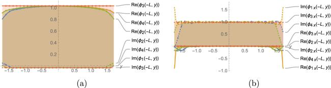
Figure 3. The real and imaginary parts of the (a) magnetic and (b) electric fields at x = − L, − h < y < h. |
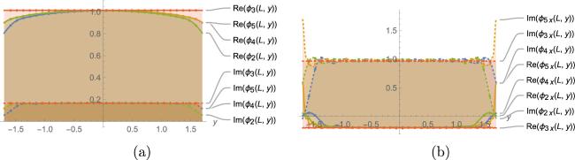
Figure 4. The real and imaginary parts of the (a) magnetic and (b) electric fields at x = L, − h < y < h. |
The behavior of the first three incident modes of reflection and transmission coefficients against the normalized frequency bω/c are presented in figures 5 and 6. It is worthwhile to mention that the region where the angular frequency ω is less than the plasma frequency ωp is termed as the non-transparency region (ω < ωp), and the region where ω is greater than ωp is called the transparency region (ω > ωp).
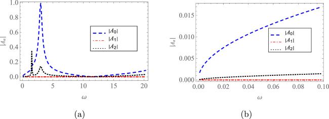
Figure 5. Reflected coefficients ∣An∣ in the (a) transparency and (b) non-transparency regions. |
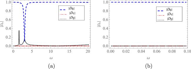
Figure 6. Transmitted coefficients ∣Dn∣ in the (a) transparency and (b) non-transparency regions. |
In terms of the normalized frequency, bω/c is considered higher than 0.1 (bω/c > 0.1) in the transparency region, while it is lower than 0.1 (bω/c < 0.1) in the non-transparency region.
The graphs of reflected and transmitted powers are revealed in figures 7-9. The reflected power in the left duct (x < − L) is represented by ${{ \mathcal E }}_{1}.$ The quantity ${{ \mathcal E }}_{2}$ is the transmitted power in the right duct (x > L). Here, ${{ \mathcal E }}_{t}$ is the sum of powers in all duct regions,
$\begin{eqnarray*}{{ \mathcal E }}_{t}={{ \mathcal E }}_{1}+{{ \mathcal E }}_{2}.\end{eqnarray*}$
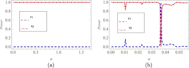
Figure 7. Power flux plotted against height a in (a) the transparency region and (b) the non-transparency region. |
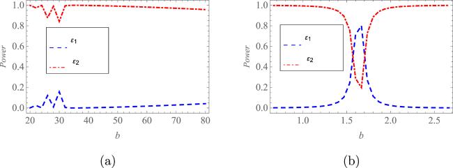
Figure 8. Power flux plotted against height b in (a) the transparency region and (b) the non-transparency region. |
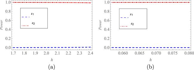
Figure 9. Power flux plotted against h in (a) the transparency and (b) the non-transparency regions. |
Figure 10 displays the plot of reflected and transmitted powers against the number of terms.
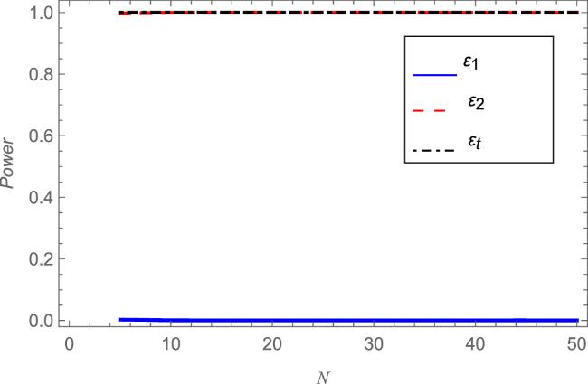
Figure 10. Power flux plotted against truncated terms N. |
The relevant duct heights are set to $\overline{b}=1\,\mathrm{cm}$, $\overline{a}=0.004\,\mathrm{cm}$, $\overline{h}=0.085\,\mathrm{cm}$. The length of the groove is fixed as $2\overline{L}=2\times 0.005\,\mathrm{cm}$, while the plasma frequency is fixed to be ωp = 109. The values of $\overline{a},\overline{b}$ and ωp are consistent with Najari et al [38]. The quantities a, b, h and L are the non-dimensional counterparts of $\bar{a},\bar{b},\bar{h}$ and $\overline{L},$ respectively. It is important to note that for all the plots other than the incident modes, the angular frequency is considered as ω = 6 × 10⁹.
The reconstruction of matching conditions of the magnetic field φi and the electric field ${\phi }_{{ix}}=\displaystyle \frac{\partial {\phi }_{i}}{\partial x},\,i=1,2,3,4$ at the interface x = -L is shown in figures 3(a) and (b). The real and imaginary parts of these fields completely coincide at this interface. Figure 4(a) indicates the excellent agreement of real and imaginary parts of the magnetic field φj, j = 2, 3, 4, 5, while figure 4(b) shows cogency of these components of the electric field ${\phi }_{{jx}}=\displaystyle \frac{\partial {\phi }_{j}}{\partial x}$ at the interface x = L.
Cut-on modes with respect to the heights a, b and h, in all regions of the waveguide, for the transparency regime are also calculated. Region 1 represents the left duct x < − L, ∣y∣ ≤ h. The regions −b ≤ y ≤ − a or a ≤ y ≤ b in ∣x∣ < L are represented as region 2, while region −a ≤ y ≤ a, comprising cold plasma, is considered as region 3. The right duct x > L, ∣y∣ ≤ h is considered as region 4.
With the increase in height h, regions 1 and 4 exhibit two cut-on modes. In region 2, the dielectric has five while, in region 3, cold plasma has only one cut-on mode. Tables 1 and 2 represent the cut-on modes with respect to heights a and b, respectively. Figures 7(a), 8(a) and 9(a) display the behavior of energy flux against the respective duct heights a, b and h in the transparency regime. Figures 7(b), 8(b) and 9(b) present this behavior in the non-transparency regime. These figures conclude that the power balance identity (equation (65 )), mentioned in section 4 , is achieved by the mode-matching solution for varying duct heights. The differences in the transparency and non-transparency regions are noticed as differences in heights only. It is observed from the figures that total transmission takes place with respect to the increase in heights. The only fluctuation in transmission is observed in heights a and b in the non-transparency regime.
Table 1. Cut-on modes. |
| Height (a) | Region 1 | Region 2 | Region 3 | Region 4 |
|---|---|---|---|---|
| 0.02 | 2 | 5 | 1 | 2 |
| 1.6 | 2 | 5 | 2 | 2 |
Table 2. Cut-on modes. |
| Height (b) | Region 1 | Region 2 | Region 3 | Region 4 |
|---|---|---|---|---|
| 20 | 2 | 7 | 1 | 2 |
| 24 | 2 | 8 | 1 | 2 |
Table 3. Convergence through truncation. |
| Terms (N) | ${{ \mathcal E }}_{1}$ | ${{ \mathcal E }}_{2}$ | ${{ \mathcal E }}_{t}$ |
|---|---|---|---|
| 5 | 0.002 922 | 0.997 078 | 1 |
| 10 | 0.000 951 | 0.999 049 | 1 |
| 15 | 0.000 624 | 0.999 376 | 1 |
| 20 | 0.000 760 | 0.999 240 | 1 |
| 25 | 0.000 746 | 0.999 254 | 1 |
| 30 | 0.000 783 | 0.999 217 | 1 |
| 35 | 0.000 816 | 0.999 184 | 1 |
| 40 | 0.000 817 | 0.999 183 | 1 |
| 45 | 0.000 847 | 0.999 153 | 1 |
| 50 | 0.000 847 | 0.999 153 | 1 |
For the graphs plotted against heights, the values of $\overline{a},\overline{b}$ and $\overline{h}$ are considered between $0.001\lt \overline{a}\lt 0.084\,\mathrm{cm}$, $1\lt \overline{b}\lt 4$ and $0.085\lt \overline{h}\lt 0.12,$ respectively. Figure 10 depicts the variation of the modulus of powers versus the truncation number N. It is evident from the figure, as well as table 3, that the effect of the truncation is insignificant for N ≥ 45. Therefore, the infinite system of algebraic equations for this case can be easily dealt with as finite.
5.2. Case II
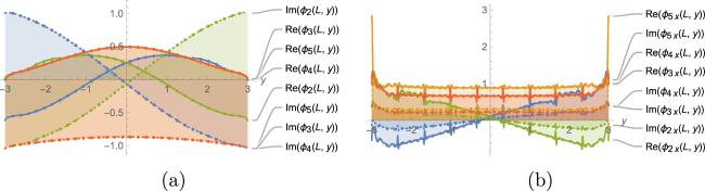
To establish the validity of the proposed solution and to provide physical insight into the given problem, the system revealed in equations (47 ), (48 ), (54 ) and (55 ) is truncated up to 70 terms. Figures 11(a) and (b) reflect the cogency of real and imaginary parts of the magnetic field φi and the electric field ${\phi }_{{ix}}=\displaystyle \frac{\partial {\phi }_{i}}{\partial x},\,i=1,2,3,4$ at the interface x = − L. The perfect agreement of the components of these fields φj and ${\phi }_{{jx}}=\displaystyle \frac{\partial {\phi }_{j}}{\partial x},\,j=2,3,4,5$ at the interface x = L is exhibited in figures 12(a) and (b). It is obvious that the truncated solution reconstructs the matching conditions of the magnetic and electric fields.
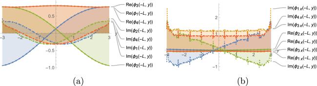
Figure 11. The real and imaginary parts of the (a) magnetic and (b) electric fields at x = − L, − h < y < h. |
Figure 12. The real and imaginary parts of the (a) magnetic and (b) electric fields at x = L, − h < y < h. |
The duct heights are specified as $\overline{b}=0.5\,\mathrm{cm}$, $\overline{a}=0.4\,\mathrm{cm}$, $\overline{h}=0.45\,\mathrm{cm}$. The length of the groove is set to $2\overline{L}=2\times 0.42\,\mathrm{cm}$. The plasma frequency is fixed as ωp = 109.
6. Concluding remarks
A detailed investigation of the propagation of electromagnetic waves in a parallel-plate rectangular waveguide with a groove, with a slab of cold plasma in its center, has been conducted. The study was focused to investigate a structure with a view to its use as a plasma waveguide resonator and gas chromatography equipment. These designs can also be applied in plasma antennas, halfway plates and frequency selective surfaces. The reflection and transmission analysis in this paper may find use in reflective-type halfway plates and transmission control in quarter-wave plate and half-wave plate metallic and all-dielectric metasurfaces [44, 45]. The physical configuration includes a groove enclosed between two semi-bounded waveguides. The left and right sections of the waveguide were composed of semi-bounded regions x < − L and x > L, respectively, with a metallic wall of height 2h and with a dielectric. The central section is a bounded metallic groove ∣x∣ < L, with height 2b. It contains a slab of cold plasma, with height 2a, (I) bounded by metallic strips, and (II) embedded between dielectric layers without metallic strips. The boundary value problems corresponding to reflection and transmission for both cases were formed into systems of infinite algebraic equations.
The results obtained for case (I) were compared with numerical deductions presented by Najari et al. The mode-matching solution was explored to analyze the behavior of transmission and reflection coefficients for the first three incident modes in the transparency and non-transparency regimes. The first mode of the reflected wave remains dominant in the transparency and non-transparency regimes. It is also concluded that the first transmitted mode is dominant in both frequency regimes. The magnitudes of the reflection and transmission coefficients for modes other than the dominant mode are negligible in the non-transparency region.
The energy flux in different duct sections is also analyzed for both transparency and non-transparency cases. The energy propagates for both cases with the changes in the heights of the waveguide, while reflection remains negligible with the increase in the heights. The conservation of power establishes the convergence and accuracy of the proposed solution.
This work can be extended in the form of a symmetric rectangular waveguide with more than one plasma slab embedded between metallic conducting plates or dielectric layers inside the groove. A structure with periodic grooves with plasma slabs sandwiched between layers of dielectric material can also be discussed.