


1. Introduction
The coexistence of superfluid and density order is usually thought to be exotic. The reason is that the density order usually means lack of mobility and superfluidity means dissipativeless flow where mobility is strong. However, closer scrutiny tells us a density-ordered superfluid is a condensation that happens at a finite momentum, which makes it less contradictory. This kind of phase can be achieved by competition between short-range and long-range interactions [1-8], such as in cavity Bose-Einstein condensate (BEC) systems [9-13], in dipolar gases systems [14-17], or by dispersion modification such as the stripe phase in BEC with spin-orbit-coupling [18-24]. Among these mechanisms, either we need a finite-range interaction or a dispersion modification to locate kinetic energy minimal to a finite momentum state. Here, we try to go beyond these two mechanisms.
In this paper, we give an example of a density ordered superfluid phase by the competition between frustrations and local interactions. To be more specific, we find a homogenous Mott insulator (MI) to density wave ordered superfluid (DWSF) transition in a frustrated triangle lattice system with interacting bosons. The Bose-Hubbard model (BHM) on a triangular lattice with positive hopping strength is well studied previously. A connection is found between the frustrated BHM and the Kosterlitz-Thouless (KT) phase. A 120-degree chiral order is developed to reconcile the requirement of the homogeneous phase by strong local interactions and the sign structure required by frustration, but no density order is presented [25]. It seems that the presence of frustrations and local interactions is not enough for a DWSF. However, a DWSF is generated to avoid frustration when we add an on-sie pairing term [26]. Practically, these on-site pairing terms are natural in Kerr cavity systems [27], exciton-polariton systems [28, 29] as well as in the nuclear magnetic resonance (NMR) systems with an anti-squeezing technique [30]. The previous work focuses on a weak interaction region where a homogeneous MI to DWSF transition is missing. Here in this paper, we study the Mott region and find a homogeneous MI to DWSF transition, which justifies the density order being emergent from spontaneously symmetry breaking (SSB).
In the following, we will first present our model and then we give the phase diagram by a standard mean-field theory method. Then we study the transition mechanism by an effective theory. We find three typical phase transitions as we increase the frustration with fixed pairing energy. The first transition is a MI-DWSF transition. Distinct with frustrated BHM without a pairing term, this DWSF is non-chiral. The second transition is between two non-chiral DWSFs. In this transition, an emergent U(1) symmetry is found at the critical point. We call it a 'shamrock transition' because its degenerate ground state in the parameter space is a shamrock-like curve rather than a circle in an LG-type transition. The third one is a chiral symmetry broken transition where a chiral ordered DWSF is generated. Here we focus on the first two transitions (figure 1(b)). Then by perturbation expansion of order parameters, we find effective theories for MI-DWSF transition and the 'shamrock transition'. We find the shamrock transition is closely related to clock models and gives a different direction to study KT transitions.
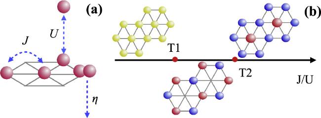
Figure 1. (a) Illustration of the model. A Bose-Hubbard model on a triangle lattice with pair generation term. (b) Typical phases for fixed η/U with increasing J/U. There are Mott insulator, non-chiral supersolid, and chiral supersolid phases. When J/U is small, the first phase is the homogenous Mott insulator phase. The yellow color in (b) means the density is homogenous. Between T1 and T2, there is a supersolid phase. The red and blue mean these bosons are condensed in opposite phase 0 and π. There is a density order as the superfluid density is only nonzero on the rings of the triangle lattice. As in this phase, the chiral symmetry is not broken. Thus, we name it as a non-chiral supersolid phase. There is no superfluid density in the hexagon center. When J/U > T2, then the system turns to a different supersolid phase. In this phase, the phase 0 atoms are condensed in the hexagon center and have a larger density. The phase π condensation is shown in blue on the rings of the hexagon with a smaller superfluid density. Here it is also a non-chiral superfluid. At J/U = T2, the transition is first order, and the system rotates from one kind of non-chiral supersolid to another non-chiral supersolid. Here we find this transition is very special, and there is an emergent U(1) symmetry at the transition point. |
2. Model
Here we consider a BHM on a triangular lattice with an on-site pairing term,
$\begin{eqnarray}\hat{H}={\hat{H}}_{\mathrm{BH}}+{\hat{H}}_{\mathrm{PR}},\end{eqnarray}$
where $\begin{eqnarray}\begin{array}{l}{\hat{H}}_{\mathrm{BH}}=J\displaystyle \sum _{\langle {ij}\rangle }({\hat{a}}_{i}^{\dagger }{\hat{a}}_{j}^{}+{\hat{a}}_{j}^{\dagger }{\hat{a}}_{i})\\ \,-\displaystyle \sum _{i}\left(\mu {\hat{n}}_{i}-\displaystyle \frac{U}{2}{\hat{n}}_{i}({\hat{n}}_{i}-1)\right),\\ {\hat{H}}_{\mathrm{PR}}=-\eta \displaystyle \sum _{i}({\hat{a}}_{i}{\hat{a}}_{i}+{\hat{a}}_{i}^{\dagger }{\hat{a}}_{i}^{\dagger }).\end{array}\end{eqnarray}$
Here ${\hat{a}}_{i}$ is an annihilation operator of a boson on site i of a triangle lattice, J > 0 is the positive hopping strength, μ is the chemical potential, U > 0 is the on-site interaction strength of bosons and η is the local pairing strength. Here we stress that for negative hopping strength J < 0, the bosons would like to have the same phase, thus there is no frustration. However, if J > 0, the hopping term requires anti-parallel phases of bosons. This requirement causes frustration in the boson model. ${\hat{n}}_{i}\,=\,{\hat{a}}_{i}^{\dagger }{\hat{a}}_{i}^{}$ is the particle number on site i, ⟨ij⟩ represents i and j are the nearest neighbors. Here we stress that the presence of η term breaks particle number conservation, thus we are not discussing Bose atoms systems but photonic systems or polariton systems.Before we dive into the details of the ground state properties of equation (1 ), let us first analyze its symmetry. One can see there is a translational symmetry on the lattice sites. Besides, there is a U(1) symmetry if η = 0, which is an invariance under transformation ${\hat{a}}_{i}\,\to \,{\hat{a}}_{i}{e}^{i\theta }$. It is broken to a Z2 symmetry ${\hat{a}}_{i}\,\to \,\pm {\hat{a}}_{i}$ when the pairing term is added. In this sense, the superfluid breaks a Z2 symmetry rather than a U(1) symmetry. Although there is no particle number conservation, there is still a charge gap in the MI phase, and there is no long-range correlation between particle annihilation and particle creation. In this sense, the concepts of the Mott insulator and superfluid are slightly modified, but are still well-defined.
3. Mean field theory and phase diagram
Now we apply a mean field theory to the Hamiltonian equation (1 ). First, we propose a mean field Hamiltonian ${\hat{H}}_{\mathrm{MF}}$ as follows,
$\begin{eqnarray}\begin{array}{l}{\hat{H}}_{\mathrm{MF}}=\displaystyle \sum _{i}\left({\hat{{ \mathcal H }}}_{i}+({\varphi }_{i-1}^{* }+{\varphi }_{i+1}^{* }){\hat{a}}_{i}\right.\\ \left.\,+\,({\varphi }_{i-1}+{\varphi }_{i+1}){\hat{a}}_{i}^{\dagger }\right),\end{array}\end{eqnarray}$
$\begin{eqnarray}\begin{array}{l}{\hat{{ \mathcal H }}}_{i}=-\mu {\hat{n}}_{i}+\displaystyle \frac{U}{2}{\hat{n}}_{i}({\hat{n}}_{i}-1)\\ \,-\,\eta ({\hat{a}}_{i}{\hat{a}}_{i}+{\hat{a}}_{i}^{\dagger }{\hat{a}}_{i}^{\dagger }),\end{array}\end{eqnarray}$
where i ∈ {1, 2, 3} are sites indices in a unit cell with three sites in it, φ = (φ1, φ2, φ3) are complex order parameters. The addition and subtraction in {1, 2, 3} are cyclonic, which means 1 − 1 = 3, 3 + 1 = 1. Now we suppose the eigenstate of ${\hat{H}}_{\mathrm{MF}}$ is ∣gφ⟩. We take this solution as an ansatz of the original Hamiltonian's ground state. Then we can obtain the ground state energy as $\begin{eqnarray}{E}_{g}=\langle {g}_{{\boldsymbol{\varphi }}}| \hat{H}| {g}_{{\boldsymbol{\varphi }}}\rangle .\end{eqnarray}$
By minimizing ground state energy Eg, then we obtain the mean field solution for φi = 1, 2, 3 by equations
$\begin{eqnarray}{\varphi }_{i}=3J\langle {g}_{{\boldsymbol{\varphi }}}| {\hat{a}}_{i}| {g}_{{\boldsymbol{\varphi }}}\rangle .\end{eqnarray}$
To better describe the order parameters, we find a decomposition as follows, $\begin{eqnarray}\begin{array}{l}{\boldsymbol{\varphi }}={{\boldsymbol{\varphi }}}^{R}+{{\boldsymbol{\varphi }}}^{I},\\ {{\boldsymbol{\varphi }}}^{R}={{\rm{\Delta }}}_{0}^{R}{\hat{\varphi }}_{0}+{{\rm{\Delta }}}_{+}^{R}{\hat{\varphi }}_{+}+i{{\rm{\Delta }}}_{-}^{R}{\hat{\varphi }}_{-},\\ {{\boldsymbol{\varphi }}}^{I}=i{{\rm{\Delta }}}_{0}^{I}{\hat{\varphi }}_{0}\ +i{{\rm{\Delta }}}_{+}^{I}{\hat{\varphi }}_{+}-{{\rm{\Delta }}}_{-}^{I}{\hat{\varphi }}_{-},\end{array}\end{eqnarray}$
where ${\hat{\varphi }}_{0}\,=\,(1,\,1,\,1)/\sqrt{3}$, ${\hat{\varphi }}_{+}\,=\,(2,\,-1,\,-1)/\sqrt{6}$, and ${\hat{\varphi }}_{-}\,=\,(0,\,1,\,-1)/\sqrt{2}$ are three unit vectors. We introduce ${{\rm{\Delta }}}_{0}\,=\,{{\rm{\Delta }}}_{0}^{R}\,+\,i{{\rm{\Delta }}}_{0}^{I}$, ${{\rm{\Delta }}}_{\pm }\,=\,{{\rm{\Delta }}}_{\pm }^{R}\,+\,i{{\rm{\Delta }}}_{\pm }^{I}$, where ${{\rm{\Delta }}}_{\pm }^{R}$, ${{\rm{\Delta }}}_{\pm }^{I}$ and ${{\rm{\Delta }}}_{0}^{R,I}$ are real. A self-consistent numerical solution can be obtained and we show Δ0, and Δ± for different J/U and fixed μ/U = 2.875 and η/U = 0.06 in figure 2.
Figure 2. A typical order parameter evolution over J/U when η/U = 0.06 and μ/U = 2.875 are fixed. In (a), we show a solution for φI = 0, φR ≠ 0 (superfluid A). The blue line is for ${{\rm{\Delta }}}_{-}^{R}$, the red dashed line is for ${{\rm{\Delta }}}_{+}^{R}$ and the green dot-dashed line is for ${{\rm{\Delta }}}_{0}^{R}$. In (b), we show another solution for φR = 0, φI ≠ 0 (superfluid B). The blue line is for ${{\rm{\Delta }}}_{-}^{I}$, the red dashed line is for ${{\rm{\Delta }}}_{+}^{I}$ and the green dot-dashed line is for ${{\rm{\Delta }}}_{0}^{R}$. Finally, in (c), we show the energy difference ΔEg between superfluid A and superfluid B. ΔEg < 0 means that the superfluid B phase has a lower energy. From the order parameter diagram, we can read for small J/U, it is a Mott insulator which we label as phase I. As J/U becomes larger, superfluid B is favorable. ${{\rm{\Delta }}}_{-}^{I}\,\ne \,0$ and all other order parameters are zero. When J/U further increases, a first order transition happens from superfluid B to superfluid A, where ${{\rm{\Delta }}}_{+}^{R}\,\ne \,0$ and ${{\rm{\Delta }}}_{0}^{R}\,\ne \,0$. Then when J/U increases further, the non-chiral superfluid A will transition to chiral superfluid A where ${{\rm{\Delta }}}_{+}^{R}\,\ne \,0$, ${{\rm{\Delta }}}_{0}^{R}\,\ne \,0$ and ${{\rm{\Delta }}}_{-}^{R}\,\ne \,0$. When all these three parameters are non-zero, the order parameter is complex and thus breaks the chiral symmetry. |
One can find that there is a symmetry for three sites permutation in the unit cell. Therefore ${\hat{\varphi }}_{+}$ mode should be equivalent to $(-1,\,2,\,-1)/\sqrt{6}$ and $(-1,-1,2)/\sqrt{6}$. For simplicity, let us first neglect this Z3 permutation symmetry and we will come back to this point later. In the mean-field theory, we find the superfluid solution can be either φR ≠ 0, φI = 0 (superfluid A) or φI ≠ 0, φR = 0 (superfluid B). In figure 2(a), we show the order parameters of φR in the superfluid A phase. In this state, ${{\rm{\Delta }}}_{+}^{R}$ and ${{\rm{\Delta }}}_{0}^{R}$ become nonzero first. When ${{\rm{\Delta }}}_{-}^{R}\,=\,0$, time-reversal symmetry is not broken. While ${{\rm{\Delta }}}_{-}^{R}$ becomes nonzero, φR is complex, then chiral symmetry is broken. In figure 2(b) we show the order parameters of φI in the superfluid B phase. In this state, ${{\rm{\Delta }}}_{-}^{I}$ emerges first while ${{\rm{\Delta }}}_{+}^{I}$ and ${{\rm{\Delta }}}_{0}^{I}$ follow. Finally, in figure 2(c), we show the energy difference between two superfluid states. The ground state of the system is then these two DWSFs with lower energy. The system goes through a second-order transition when the order parameters become nonzero within a single state. The level crossing between superfluid A and superfluid B is the 'shamrock transition' we mentioned before.
To be more specific, we explain how these phase transitions happen following figure 2, which is along the arrow line in the phase diagram given in figure 3(b). (1) Mott insulator phase with all superfluid order parameters φ = 0 (phase I). The density is homogeneous in this phase. (2) As J/U increases, the system goes through a MI-DWSF transition where a condensation in ${\hat{\varphi }}_{-}$ mode happens with ${{\rm{\Delta }}}_{-}^{I}\,\ne \,0$ only. In this phase, the system is in DWSF at ${\hat{\varphi }}_{-}$ mode (phase II). As mode $(1,-1,0)/\sqrt{2}$ and $(1,0,-1)/\sqrt{2}$ are equivalent to ${\hat{\varphi }}_{-}$ mode and the system has a parity symmetry in ${{\rm{\Delta }}}_{-}^{I}$. Together the symmetry is Z3 × Z2 = Z6. The case we show here is only one possibility. (3) As J/U further increases, a level crossing happens, the condensation rotates from ${\hat{\varphi }}_{-}$ mode to a combination of ${\hat{\varphi }}_{0}$ and ${\hat{\varphi }}_{+}$ mode (phase V). (4) An even larger J/U induces a chiral symmetry broken, all three order parameters of φR are nonzero (phase IV). This phase is a chiral ordered superfluid.
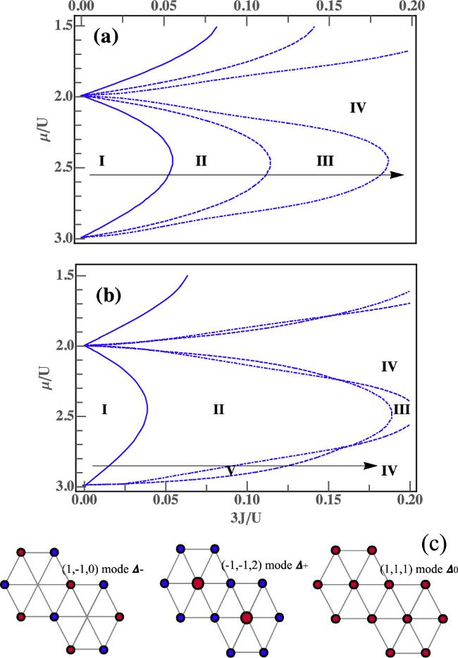
Figure 3. Phase diagram of the Bose-Hubbard model with pairing term. In (a) we fixed η/U = 0.025. The phase diagram is presented for μ/U ∈ [1.5, 3] and J/U ∈ [0, 0.0667]. There are in total 4 types of phases. I for Mott insulator, II for non-chiral superfluid B, III for chiral ordered superfluid B and IV for chiral ordered superfluid A. In (b), η/U = 0.06, there is one phase more, V stands for non-chiral superfluid A. The relation between these phases and the order parameters are the following. In the Mott phase I, φ = 0. The other phases are all superfluid density-ordered phases. The configuration of the non-chiral supersolid phase and the chiral supersolid phase are shown in figure 1(b). Mainly, it is about whether the order parameter must be complex. The order parameter φ = φR + φI is further decomposed into ${{\rm{\Delta }}}_{0}^{R/I}$, ${{\rm{\Delta }}}_{+}^{R/I}$ and ${{\rm{\Delta }}}_{-}^{R/I}$, as are shown in (c). In supersolid II, ${{\rm{\Delta }}}_{-}^{I}\ne 0$, ${{\rm{\Delta }}}_{-}^{I}\,=\,{{\rm{\Delta }}}_{0}^{I}\,=\,{{\boldsymbol{\varphi }}}^{R}=0$. Clearly, phase II is non-chiral supersolid B. In superfluid III, ${{\rm{\Delta }}}_{+}^{I}\,\ne \,0$, ${{\rm{\Delta }}}_{-}^{I}\,\ne \,0$, ${{\rm{\Delta }}}_{0}^{I}\,\ne \,0$ and φR = 0. As the order parameter is complex, the superfluid phase breaks the chiral symmetry. This is chiral supersolid B. In phase IV, ${{\rm{\Delta }}}_{\pm }^{R}\,\ne \,0$, ${{\rm{\Delta }}}_{0}^{R}\,\ne \,0$, and φI = 0. This is the chiral superfluid A phase. Finally, in phase V, ${{\rm{\Delta }}}_{+}^{R}\,\ne \,0$, ${{\rm{\Delta }}}_{0}^{R}\,\ne \,0$, ${{\rm{\Delta }}}_{-}^{R}\,=\,0$ and φI = 0. This is non-chiral superfluid A phase. |
Following the calculations for the order parameters, we can then draw a phase diagram for fixed η/U, varying μ/U and J/U. The total phase diagram is shown in figure 3(a) and (b). Compared with the phase diagram at η/U = 0, there are inhomogeneous density ordered superfluid phases with, or without chiral order. It shows that a density-ordered superfluid is possible under the competition between frustration and the local interactions.
4. Mechanism study
Now, we try to understand the phase transitions and figure out the mechanism. Here η term is taken as a perturbation. Based on equation (7 ), we find up to the second order of φ, the ground state energy Eg can be expressed as
$\begin{eqnarray}\begin{array}{l}{E}_{g}^{(2)}=\displaystyle \sum _{\sigma =\pm }{\chi }_{\sigma }\left(1-6J{\chi }_{\sigma }\right)\left({\left({{\rm{\Delta }}}_{\sigma }^{R}\right)}^{2}+{\left({{\rm{\Delta }}}_{-\sigma }^{I}\right)}^{2}\right)\\ \,+{\chi }_{+}\left(1+6J{\chi }_{+}\right){\left({{\rm{\Delta }}}_{0}^{R}\right)}^{2}\\ \,+{\chi }_{-}\left(1+6J{\chi }_{-}\right){\left({{\rm{\Delta }}}_{0}^{I}\right)}^{2},\end{array}\end{eqnarray}$
where ${\chi }_{\pm }=\chi \pm 2\eta \chi ^{\prime} $, and $\begin{eqnarray}\chi =\displaystyle \frac{{\ell }+1}{{\epsilon }_{{\ell }+1}-{\epsilon }_{{\ell }}}+\displaystyle \frac{{\ell }}{{\epsilon }_{{\ell }-1}-{\epsilon }_{{\ell }}},\end{eqnarray}$
$\begin{eqnarray}\begin{array}{l}\chi ^{\prime} =\displaystyle \frac{({\ell }+1)({\ell }+2)}{({\epsilon }_{{\ell }}-{\epsilon }_{{\ell }+1})({\epsilon }_{{\ell }}-{\epsilon }_{{\ell }+2})}\\ \,+\,\displaystyle \frac{{\ell }({\ell }+1)}{({\epsilon }_{{\ell }}-{\epsilon }_{{\ell }+1})({\epsilon }_{{\ell }}-{\epsilon }_{{\ell }-1})}\\ \,+\,\displaystyle \frac{{\ell }({\ell }-1)}{({\epsilon }_{{\ell }}-{\epsilon }_{{\ell }-1})({\epsilon }_{{\ell }}-{\epsilon }_{{\ell }-2})}.\end{array}\end{eqnarray}$
Here ℓ = ⌊μ/U⌋ is the integer part of μ/U. εℓ = − μℓ + Uℓ(ℓ − 1)/2. We find in general χ− < χ+ as long as η > 0. Therefore there are three typical regions for hopping strength J, that is, region (i) (χ− < χ+ < 1/6J), region (ii) (χ− < 1/6J < χ+), and region (iii) (1/6J < χ− < χ+). In region (i), all coefficients are positive so the order parameters are zero, which corresponds to the MI phase. In region (ii), only ${{\rm{\Delta }}}_{+}^{R}$ or ${{\rm{\Delta }}}_{-}^{I}$ can be nonzero, where a density order related to ${\hat{\varphi }}_{+}$ or ${\hat{\varphi }}_{-}$ mode is spontaneously generated. Meanwhile, a superfluid order is developed with nonzero φ. Finally, in region (iii), the order parameter becomes complex such that a chiral order is developed.We will only focus on the transitions in region (i) and (ii). In these regions, only order parameters ${{\rm{\Delta }}}_{-}^{I}$, ${{\rm{\Delta }}}_{+}^{R}$ and ${{\rm{\Delta }}}_{0}^{R}$ are important. To better describe our problem, we introduce three real order parameters $\varphi \,\in \,{\mathbb{R}}$, θ ∈ S1, and $\phi \,\in \,{\mathbb{R}}$, where ${{\rm{\Delta }}}_{-}^{I}\,=\,\varphi \cos \theta $, ${{\rm{\Delta }}}_{+}^{R}\,=\,\varphi \sin \theta $ and ${{\rm{\Delta }}}_{0}^{R}\,=\,\phi $. Then we find the MI-DWSF transition is described by an effective theory as,
$\begin{eqnarray}{E}_{g}\approx {u}_{2}{\varphi }^{2}+{u}_{4}{\varphi }^{4}+{u}_{6}{\varphi }^{6}-{u}_{6}^{{\prime} }{\varphi }^{6}\cos 6\theta ,\end{eqnarray}$
where u2, u4, u6, ${u}_{6}^{{\prime} }$ are phenomenological parameters [31]. At zero temperature, the MI-DWSF transition is characterized by sign change in u2 with u4 > 0, u6 > 0 and ${u}_{6}^{{\prime} }\,\gt \,0$. Here as ${u}_{6}^{{\prime} }\,\gt \,0$, therefore ${{\rm{\Delta }}}_{-}^{I}\,\ne \,0$, ${{\rm{\Delta }}}_{+}^{R}\,=\,0$ is a solution.In region II, let us assume that the superfluid order is large enough that we can neglect the fluctuations of the magnitude mode of φ, then we find the effective ground state energy can be written as [31] 12 ) that at the transition point, the ground state energy does not have θ dependence, therefore a U(1) symmetry is emergent at the transition point. As we see the energy minima lies in a shamrock-like curve. Therefore we call the transition a 'shamrock transition'. The transition is special in two ways. First, although the order parameter jumps at the transition point, the emergent symmetry may result in some special quantum criticality. On the other hand, no symmetry is broken across the transition, therefore it is neither a spontaneously symmetry broken transition. For this reason, the 'shamrock transition' is beyond the LG paradigm and deserves further study.
$\begin{eqnarray}{E}_{g}=-u\cos 6\theta +\lambda \phi \sin 3\theta +{m}^{2}{\phi }^{2}.\end{eqnarray}$
When u > 0, θ = 2nπ/6, n = 0, 1, 2, 3, 4, 5 are ground state manifold solutions. This solution is just ${{\rm{\Delta }}}_{-}^{I}\,\ne \,0$ DWSF, a condensation in ${\hat{\varphi }}_{-}$ mode. On the other hand, when u < λ2/8m2, $\phi \,=\,-\lambda \sin 3\theta /2{m}^{2}$, we should take $\cos 6\theta \,=\,-1$, where θ = (2n + 1)π/6, such that $\sin 3\theta \,=\,\pm 1$. This is the other metastable solution in our calculation as ${{\rm{\Delta }}}_{+}^{R}\,\ne \,0$, ${{\rm{\Delta }}}_{0}^{R}\,\ne \,0$. The picture for this phase transition is shown in figures 4(a)-(c), where φ is put in polar direction and θ is put in angle direction. One can see in figure 4(a), the ground state takes φ = 0 and θ = nπ/3. As λ increases, in figure 4, the vacuum becomes φ > 0, and $\theta \,=\,\tfrac{\pi }{2},\tfrac{7\pi }{6},\tfrac{11\pi }{6}$ or φ < 0, $\theta \,=\,\tfrac{\pi }{6},\tfrac{5\pi }{6},\tfrac{3\pi }{2}$. One can observe from figure 4(b) or from equation (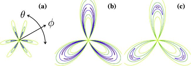
Figure 4. Cross sections of the energy curve for equation ( |
The effective theory given in equation (12 ) is in the same universality class of the six-state clock model [32-36], and it enables us to have some guesses for finite temperature phases. For d = 2 (d is the spatial dimension), if the system doesn't have particle-hole symmetry, then the total dimension D is still 2 (D is the quantum dimension). Then when the temperature rises, the system first goes through a first-order transition from DWSF to a KT phase with a recovered U(1) symmetry. As the temperature continues to increase, the KT superfluid phase becomes a disordered phase. Although it may not be so surprising from an effective field theory view, the U(1) symmetry here is quite different from the original U(1) symmetry. Under this U(1) symmetry, the density pattern can rotate from (0, 1, −1) mode to (2, −1, −1) mode, which seems to be a very exotic non-homogeneous superfluid. If there is particle-hole symmetry, the ${\left({\partial }_{\tau }\theta \right)}^{2}$ term becomes the leading order in the effective action, therefore the total dimension becomes three. In three-dimensional space, there is only one transition from the ordered phase to disordered phase. Therefore we expect a critical line to start from the quantum critical point which separates superfluid A and superfluid B.
5. Conclusion and outlook
To summarize, we have proved that a DWSF is possible due to the competition between frustrations and local interactions. In the modified Bose-Hubbard model on a triangle lattice, a Mott insulator phase, and four DWSFs are discovered by the mean-field theory. An interesting transition (the shamrock transition) between two non-chiral DWSFs is discovered where an emergent U(1) symmetry is presented at the critical point while both phases on each side have a Z6 symmetry. This model can be realized in Kerr cavities or exciton-polariton systems. It is a good platform for density-ordered superfluid studies and KT transition studies. Different from frustrated spin systems, the Higgs modes are unlocked in the present system. It is also a good platform to study Goldstones with light masses. Many new physics are generated due to the unlocked amplitude fluctuations.
Acknowledgments
We would like to thank Shaokai Jian and Shuai Yin for the valuable discussions. Y C and C W are supported by the Beijing Natural Science Foundation (Z180013) (YC), National Natural Science Foundation of China (NSFC) under Grant No. 12174358 (YC) and No. 11734010 (YC and CW), and MOST Grant No. 2016YFA0301600 (CW).
Appendix A. Effective theory at φ's second order and η's first order
The mean field Hamiltonian is
$\begin{eqnarray}{\hat{H}}_{\mathrm{MF}}=\displaystyle \sum _{j=1,2,3}{\hat{H}}_{0,j}+{\hat{V}}_{j},\end{eqnarray}$
$\begin{eqnarray}{\hat{H}}_{0,j}=-\mu {\hat{n}}_{j}+\displaystyle \frac{U}{2}{\hat{n}}_{j}({\hat{n}}_{j}-1),\end{eqnarray}$
$\begin{eqnarray}\begin{array}{l}{\hat{V}}_{j}=\eta ({\hat{a}}_{j}^{}{\hat{a}}_{j}^{}+{\hat{a}}_{j}^{\dagger }{\hat{a}}_{j}^{\dagger })\\ \,+({\varphi }_{j-1}+{\varphi }_{j+1}){\hat{a}}_{j}^{\dagger }+({\varphi }_{j-1}^{* }+{\varphi }_{j+1}^{* }){\hat{a}}_{j}.\end{array}\end{eqnarray}$
Up to φ's second order and η's first order, the ground state wave function is 8 ) in the main text.
$\begin{eqnarray}\begin{array}{l}| {\rm{\Psi }}{\rangle }_{j}=\displaystyle \frac{1}{\sqrt{{N}_{\psi }}}\left(| {\ell }\rangle +\displaystyle \sum _{{{\ell }}_{1}}\displaystyle \frac{| {{\ell }}_{1}\rangle \langle {{\ell }}_{1}| {\hat{V}}_{j}| {\ell }\rangle }{{\epsilon }_{{\ell }}-{\epsilon }_{{{\ell }}_{1}}}\right.\\ \left.\,+\displaystyle \sum _{{{\ell }}_{1},{{\ell }}_{2}}\displaystyle \frac{| {{\ell }}_{2}\rangle \langle {{\ell }}_{2}| {\hat{V}}_{j}| {{\ell }}_{1}\rangle \langle {{\ell }}_{1}| {\hat{V}}_{j}| {\ell }\rangle }{({\epsilon }_{{\ell }}-{\epsilon }_{{{\ell }}_{1}})({\epsilon }_{{\ell }}-{\epsilon }_{{{\ell }}_{2}})}\right).\end{array}\end{eqnarray}$
More explicitly, ∣$\Psi$⟩ = ∏j=1,2,3 ⨂ ∣$\Psi$⟩j is a product state of each site's wave function, where $\begin{eqnarray}\begin{array}{l}| {\rm{\Psi }}{\rangle }_{j}=| {\ell }\rangle +\displaystyle \frac{\sqrt{{\ell }+1}\varphi }{{\epsilon }_{{\ell }}-{\epsilon }_{{\ell }+1}}| {\ell }+1\rangle \\ \,+\displaystyle \frac{\sqrt{{\ell }}{\varphi }^{* }}{{\epsilon }_{{\ell }}-{\epsilon }_{{\ell }-1}}| {\ell }-1\rangle \\ \,+\displaystyle \frac{\eta \sqrt{({\ell }+2)({\ell }+1)}}{{\epsilon }_{{\ell }}-{\epsilon }_{{\ell }+2}}| {\ell }+2\rangle \\ \,+\displaystyle \frac{\eta \sqrt{{\ell }({\ell }-1)}}{{\epsilon }_{{\ell }}-{\epsilon }_{{\ell }-2}}| {\ell }-2\rangle \\ \,+\displaystyle \frac{\sqrt{({\ell }+1)({\ell }+2)}{\varphi }^{2}}{({\epsilon }_{{\ell }}-{\epsilon }_{{\ell }+1})({\epsilon }_{{\ell }}-{\epsilon }_{{\ell }+2})}| {\ell }+2\rangle \\ \,+\displaystyle \frac{\sqrt{{\ell }({\ell }-1)}{\varphi }^{* 2}}{({\epsilon }_{{\ell }}-{\epsilon }_{{\ell }-1})({\epsilon }_{{\ell }}-{\epsilon }_{{\ell }-2})}| {\ell }-2\rangle \\ \,+\displaystyle \frac{\eta \varphi ({\ell }+1)\sqrt{{\ell }}}{({\epsilon }_{{\ell }}-{\epsilon }_{{\ell }+1})({\epsilon }_{{\ell }}-{\epsilon }_{{\ell }-1})}| {\ell }-1\rangle \\ \,+\displaystyle \frac{\eta {\varphi }^{* }{\ell }\sqrt{{\ell }+1}}{({\epsilon }_{{\ell }}-{\epsilon }_{{\ell }+1})({\epsilon }_{{\ell }}-{\epsilon }_{{\ell }-1})}| {\ell }+1\rangle \\ \,+\displaystyle \frac{\eta \sqrt{{\ell }}({\ell }-1)\varphi }{({\epsilon }_{{\ell }}-{\epsilon }_{{\ell }-1})({\epsilon }_{{\ell }}-{\epsilon }_{{\ell }-2})}| {\ell }-1\rangle \\ \,+\displaystyle \frac{\eta {\varphi }^{* }({\ell }+2)\sqrt{{\ell }+1}}{({\epsilon }_{{\ell }}-{\epsilon }_{{\ell }+1})({\epsilon }_{{\ell }}-{\epsilon }_{{\ell }+2})}| {\ell }+1\rangle .\end{array}\end{eqnarray}$
Here φ is short for φj−1 + φj+1. With the help of the perturbative ground state wave function, the ground state energy can be expressed as $\begin{eqnarray}\begin{array}{l}{E}_{g}=\langle {\rm{\Psi }}| \hat{H}| {\rm{\Psi }}\rangle =\langle {\rm{\Psi }}| {\hat{H}}_{\mathrm{MF}}\\ \,-\displaystyle \sum _{j}\left(({\varphi }_{j-1}+{\varphi }_{j+1}){\hat{a}}_{j}^{\dagger }+h.c.\right)\\ \,+3J\displaystyle \sum _{j}({\hat{a}}_{j+1}^{\dagger }{\hat{a}}_{j}^{}+h.c.)| {\rm{\Psi }}\rangle \\ ={E}_{g}^{\mathrm{MF}}+\displaystyle \sum _{j}(3J\langle {\hat{a}}_{j-1}\rangle +3J\langle {\hat{a}}_{j+1}\rangle \\ \,-{\varphi }_{j-1}-{\varphi }_{j+1})\langle {\hat{a}}_{j}^{\dagger }\rangle +h.c.),\end{array}\end{eqnarray}$
where ${E}_{g}^{\mathrm{MF}}$ is the mean field ground state energy $\langle {\rm{\Psi }}| {\hat{H}}_{\mathrm{MF}}| {\rm{\Psi }}\rangle $, and $\langle {\hat{a}}_{j}\rangle \equiv \langle {\rm{\Psi }}| {\hat{a}}_{j}| {\rm{\Psi }}\rangle $. Again, the summation over j is cyclic (the summation and subtraction is module 3 in a sense 3+1 = 1). More explicitly, we have $\begin{eqnarray}\begin{array}{l}{E}_{g}^{\mathrm{MF}}=-\chi \displaystyle \sum _{j}| {\varphi }_{j-1}+{\varphi }_{j+1}{| }^{2}\\ \,-\eta \chi ^{\prime} \displaystyle \sum _{j}\left({\left({\varphi }_{j-1}+{\varphi }_{j+1}\right)}^{2}+c.c.\right),\end{array}\end{eqnarray}$
and $\begin{eqnarray}\begin{array}{l}\langle {\hat{a}}_{j}\rangle =-\chi ({\varphi }_{j-1}+{\varphi }_{j+1})\\ \,-2\eta \chi ^{\prime} ({\varphi }_{j-1}^{* }+{\varphi }_{j+1}^{* })+{ \mathcal O }({\varphi }^{3}),\end{array}\end{eqnarray}$
where $\begin{eqnarray}\chi =-\displaystyle \frac{{\ell }+1}{{\epsilon }_{{\ell }}-{\epsilon }_{{\ell }+1}}-\displaystyle \frac{{\ell }}{{\epsilon }_{{\ell }}-{\epsilon }_{{\ell }-1}},\end{eqnarray}$
$\begin{eqnarray}\begin{array}{l}\chi ^{\prime} =-\displaystyle \frac{{\ell }+1}{({\epsilon }_{{\ell }}-{\epsilon }_{{\ell }+1})}\displaystyle \frac{{\ell }+2}{{\epsilon }_{{\ell }}-{\epsilon }_{{\ell }+2}}\\ \,-\displaystyle \frac{{\ell }+1}{({\epsilon }_{{\ell }}-{\epsilon }_{{\ell }+1})}\displaystyle \frac{{\ell }}{{\epsilon }_{{\ell }}-{\epsilon }_{{\ell }-1}}\\ \,-\displaystyle \frac{{\ell }}{({\epsilon }_{{\ell }}-{\epsilon }_{{\ell }-1})}\displaystyle \frac{{\ell }-1}{{\epsilon }_{{\ell }}-{\epsilon }_{{\ell }-2}}.\end{array}\end{eqnarray}$
By introducing ${\varphi }_{1}=\tfrac{1}{\sqrt{3}}({{\rm{\Delta }}}_{0}^{R}+i{{\rm{\Delta }}}_{0}^{I})+\tfrac{2}{\sqrt{6}}({{\rm{\Delta }}}_{+}^{R}+i{{\rm{\Delta }}}_{+}^{I})$, ${\varphi }_{2}=\tfrac{1}{\sqrt{3}}({{\rm{\Delta }}}_{0}^{R}+i{{\rm{\Delta }}}_{0}^{I})-\tfrac{1}{\sqrt{6}}({{\rm{\Delta }}}_{+}^{R}+i{{\rm{\Delta }}}_{+}^{I})+$ $\tfrac{1}{\sqrt{2}}({{\rm{\Delta }}}_{-}^{R}+i{{\rm{\Delta }}}_{-}^{I})$, and ${\varphi }_{3}=\tfrac{1}{\sqrt{3}}({{\rm{\Delta }}}_{0}^{R}+i{{\rm{\Delta }}}_{0}^{I})-\tfrac{1}{\sqrt{6}}({{\rm{\Delta }}}_{+}^{R}+i{{\rm{\Delta }}}_{+}^{I})-\tfrac{1}{\sqrt{2}}({{\rm{\Delta }}}_{-}^{R}+i{{\rm{\Delta }}}_{-}^{I})$, we have $\begin{eqnarray}\begin{array}{l}{E}_{g}=\displaystyle \sum _{\sigma =\pm }{\chi }_{\sigma }\left(1-6J{\chi }_{\sigma }\right)\left({\left({{\rm{\Delta }}}_{\sigma }^{R}\right)}^{2}+{\left({{\rm{\Delta }}}_{-\sigma }^{I}\right)}^{2}\right)\\ \,+{\chi }_{+}\left(1+6J{\chi }_{+}\right){\left({{\rm{\Delta }}}_{0}^{R}\right)}^{2}\\ \,+{\chi }_{-}\left(1+6J{\chi }_{-}\right){\left({{\rm{\Delta }}}_{0}^{I}\right)}^{2},\end{array}\end{eqnarray}$
where ${\chi }_{\pm }=\chi \pm 2\eta \chi ^{\prime} $. This is the equation (Appendix B. The effective theory with real order parameters only
In some parameter regions, the order parameters are not complex. The presence of a complex order means chiral symmetry is broken. Therefore when we restrict ourselves in non-chiral superfluid, we can simplify the effective field theory.
In mean field theory, we assume the on-site Hamiltonian as
$\begin{eqnarray}\begin{array}{l}{\hat{H}}_{j}=-\mu {\hat{n}}_{j}+\displaystyle \frac{U}{2}{\hat{n}}_{j}({\hat{n}}_{j}-1)\\ \,-\eta (\hat{a}\hat{a}+{\hat{a}}^{\dagger }{\hat{a}}^{\dagger })\\ \,+\hat{a}{\left({\varphi }_{j-1}+{\varphi }_{j+1}\right)}^{* }+{\hat{a}}^{\dagger }({\varphi }_{j-1}+{\varphi }_{j+1}).\end{array}\end{eqnarray}$
Here we assume that the parameters are restricted to a phase where φj=1,2,3 are all real.First, we are going to prove that if the mean field on-site energy ${E}_{g,\mathrm{on}-\mathrm{site}}^{\mathrm{MF}}\,\equiv \,{\sum }_{j}\langle {{\rm{\Psi }}}_{g}| {\hat{H}}_{j}-{\hat{a}}_{j}^{\dagger }({\varphi }_{j-1}+{\varphi }_{j+1})-{\hat{a}}_{j}{\left({\varphi }_{j-1}+{\varphi }_{j+1}\right)}^{* }| {{\rm{\Psi }}}_{g}\rangle $ can be written in the following form, B2 ) and equation (B3 ) into equation (B5 ), and we introduce
$\begin{eqnarray}{E}_{g,\mathrm{on}-\mathrm{site}}^{\mathrm{MF}}=-\displaystyle \sum _{n=1}^{3}\displaystyle \sum _{j}{r}_{n}{\left({\varphi }_{j-1}+{\varphi }_{j+1}\right)}^{2n}+{ \mathcal O }({\varphi }^{8}),\end{eqnarray}$
Then the average of ${\hat{a}}_{j}$ must be $\begin{eqnarray}\langle {\hat{a}}_{j}\rangle =\displaystyle \sum _{n=1}^{3}({{nr}}_{n}){\left({\varphi }_{j-1}+{\varphi }_{j+1}\right)}^{2n-1}+{ \mathcal O }({\varphi }^{7}).\end{eqnarray}$
This is the result of $\partial ({\sum }_{j}\langle {\hat{H}}_{j}\rangle )/\partial ({\varphi }_{j-1}+{\varphi }_{j+1})=0$ at the extreme point. Furthermore, we find the true ground state energy ${E}_{g}=\langle \hat{H}\rangle $. In mean field approximation, it is $\begin{eqnarray}{E}_{g}={E}_{g,\mathrm{on}-\mathrm{site}}^{\mathrm{MF}}+{E}_{g,\mathrm{kin}},\end{eqnarray}$
$\begin{eqnarray}\begin{array}{l}{E}_{g,\mathrm{kin}}\equiv \langle {{\rm{\Psi }}}_{g}| J\displaystyle \sum _{\langle i,j\rangle }({\hat{a}}_{i}^{\dagger }{\hat{a}}_{j}+{\hat{a}}_{j}^{\dagger }{\hat{a}}_{i})| {{\rm{\Psi }}}_{g}\rangle \\ \,\approx J\displaystyle \sum _{\langle i,j\rangle }(\langle {\hat{a}}_{i}^{\dagger }\rangle \langle {\hat{a}}_{j}\rangle +c.c.).\end{array}\end{eqnarray}$
By inserting equation ( $\begin{eqnarray}\begin{array}{l}{\boldsymbol{\varphi }}=({\varphi }_{1},{\varphi }_{2},{\varphi }_{3})\\ \equiv \varphi \sin \theta {\hat{\varphi }}_{+}+\varphi \cos \theta {\hat{\varphi }}_{-}+\phi {\hat{\varphi }}_{0},\end{array}\end{eqnarray}$
where ${\hat{\varphi }}_{0}\,=\,(1,1,1)/\sqrt{3}$, ${\hat{\varphi }}_{+}\,=\,(2,-1,-1)/\sqrt{6}$, and ${\hat{\varphi }}_{-}\,=\,(0,1,-1)/\sqrt{2}$, we have $\begin{eqnarray}\begin{array}{l}{E}_{g}=({r}_{1}-\tilde{J}{r}_{1}^{2}){\varphi }^{2}+\left(2\tilde{J}{r}_{1}{r}_{2}-\displaystyle \frac{1}{2}{r}_{2}\right){\varphi }^{4}\\ +\displaystyle \frac{1}{36}(-28\tilde{J}{r}_{2}^{2}+10{r}_{3}-60\tilde{J}{r}_{1}{r}_{3}){\varphi }^{6}\\ +\displaystyle \frac{1}{36}(-8\tilde{J}{r}_{2}^{2}-{r}_{3}+6\tilde{J}{r}_{1}{r}_{3}){\varphi }^{6}\cos (6\theta )\\ +\displaystyle \frac{4\sqrt{2}}{3}(-{r}_{2}+\tilde{J}{r}_{1}{r}_{2})\sin (3\theta ){\varphi }^{3}\phi \\ +\sqrt{2}\left(\displaystyle \frac{4\tilde{J}}{3}{r}_{2}^{2}+\displaystyle \frac{5}{3}{r}_{3}-5\tilde{J}{r}_{1}{r}_{3}\right)\sin (3\theta ){\varphi }^{5}\phi \\ +(4{r}_{1}+8\tilde{J}{r}_{1}^{2}){\phi }^{2}+(-8{r}_{2}-16\tilde{J}{r}_{1}{r}_{2}){\phi }^{2}{\varphi }^{2}\\ +(8\tilde{J}{r}_{2}^{2}+10{r}_{3}){\varphi }^{4}{\phi }^{2},\end{array}\end{eqnarray}$
where $\tilde{J}=6J$. Here to simplify the effective theory, we find the second order coefficient of φ field is always positive. Initially, when we consider the superfluid transition, we fix φ = 0, then the effective theory is $\begin{eqnarray}{E}_{g}={u}_{2}{\varphi }^{2}+{u}_{4}{\varphi }^{4}+{u}_{6}{\varphi }^{6}-{u}_{6}^{{\prime} }{\varphi }^{6}\cos (6\theta ),\end{eqnarray}$
where ${u}_{2}={r}_{1}-\tilde{J}{r}_{1}^{2}$, ${u}_{4}=2\tilde{J}{r}_{1}{r}_{2}-\tfrac{1}{2}{r}_{2}$, ${u}_{6}=(-28\tilde{J}{r}_{2}^{2}+10{r}_{3}-60\tilde{J}{r}_{1}{r}_{3})/36$, and $u{{\prime} }_{6}=(-8\tilde{J}{r}_{2}^{2}-{r}_{3}\,+\,6\tilde{J}{r}_{1}{r}_{3})/36$. Within the superfluid phase, if we assume φ ≠ 0 is fixed, then $\begin{eqnarray}{E}_{g}=-u\cos (6\theta )+\lambda \phi \sin 3\theta +{m}^{2}{\phi }^{2},\end{eqnarray}$
where u, m2, λ are all φ dependent parameters. These parameters can be obtained when rn=1,2,3 and φ are given.