


1. Introduction
The study of interaction waves between solitons and other types of nonlinear waves is a topic of great interest in soliton theory. In recent years, there has been remarkable progress in finding the analytical solution of soliton-cnoidal waves due to the introduction of some new effective methods, such as the localization of nonlocal symmetry [1–6], the consistent Riccati expansion method [7, 8], and the consistent tanh expansion (CTE) method [9–11]. In fact, such types of interaction waves have been observed in real world and laboratory experiments. For example, it has been reported in an experimental observation that truly traveling waves, consisting of a strongly localized solitary wave residing on a small amplitude oscillatory tail, are generated from a woodpile lattice [12].
Recently, a bound state of multiple-soliton solution, called soliton molecule, has rapidly become a popular topic in both theoretical study and experimental observation, ranging from optical fibers [13, 14] to Bose–Einstein condensation [15, 16]. To construct abundant patterns of soliton molecules, Lou proposed a velocity resonance mechanism for (1+1)-dimensional fluid systems [17–21]. Based on this mechanism, soliton molecules have been discovered in several famous integrable systems [22–29], including the complex modified KdV equation [22], the (2+1)-dimensional bidirectional Sawada–Kotera system [23], and the Sharma–Tasso–Olver–Burgers system [24]. In addition, dromion molecules described by the variable separation solution were reported for the first time by applying the multilinear variable separation approach to the (3+1)-dimensional Boiti–Leon–Manna–Pempinelli system [29].
In this work, we consider the following (2+1)-dimensional modified KdV (2DmKdV) system [30]1 ) is confirmed in [30]. It is noteworthy that, as detailed in [33], Hu developed a bilinear Bäcklund transformation and a nonlinear superposition formula to the 2DmKdV system (1 ).
$\begin{eqnarray}\left\{\begin{array}{l}{u}_{t}+{u}_{{xxy}}+4\lambda {u}^{2}{u}_{y}-2{u}_{x}v+\alpha {({u}_{{xx}}+2\lambda {u}^{3})}_{x}+\beta {({u}_{{xxxx}}+6{u}^{5}+10\lambda {u}^{2}{u}_{{xx}}+10\lambda {{uu}}_{x}^{2})}_{x}=0,\\ {v}_{x}+2\lambda {{uu}}_{y}=0,\end{array}\right.\end{eqnarray}$
which reduces to the (2+1)-dimensional modified Bogoyavlenskii–Schiff equation [31, 32] for α = β = 0 and λ = –1. The existence of a three-soliton solution of the 2DmKdV system (The paper is structured as follows. In section 2 , the nonlocal residue symmetry and the Bäcklund transformation of the 2DmKdV system with λ = –1 are obtained from its truncated Painlevé expansion. Then, new auxiliary functions are introduced to localize the nonlocal symmetry to Lie point symmetry, and thus a finite transformation group is derived. In section 3, the CTE method is utilized to prove the integrablity of the 2DmKdV system with λ = –1 and to derive the interaction wave solution between one-soliton/kink and the surrounding periodic waves. In section 4, the 2DMKdV system with λ = 1 is transformed to a bilinear form and the multiple-soliton solution is presented. By imposing the velocity resonance condition on the multiple-soliton solution, abundant patterns of soliton molecules are generated. Some concluding remarks are given in the last section.
2. The truncated painlevé expansion and its related nonlocal residue symmetry
According to the truncated Painlevé expansion method, the Laurent series expansions of u and v in (1 ) read2 ) into (1 ) and then eliminating the coefficients of all different powers of φ−1 lead to the solutions of the unknown functions
$\begin{eqnarray}\begin{array}{l}u=\displaystyle \frac{{u}_{0}}{\phi }+{u}_{1},\quad v=\displaystyle \frac{{v}_{0}}{{\phi }^{2}}+\displaystyle \frac{{v}_{1}}{\phi }+{v}_{2},\end{array}\end{eqnarray}$
where u0, u1, v0, v1, v2 are undetermined functions of (x, y, t), and φ = φ(x, y, t) is the singularity manifold. Substituting ( $\begin{eqnarray}\begin{array}{l}{u}_{0}=\delta {\phi }_{x},\quad {v}_{0}={\phi }_{x}{\phi }_{y},\quad {u}_{1}=-\displaystyle \frac{\delta }{2}\displaystyle \frac{{\phi }_{{xx}}}{{\phi }_{x}},\\ \,\quad {v}_{1}=-{\phi }_{{xy}},\quad \delta =\pm 1,\\ {v}_{2}=\displaystyle \frac{1}{2}\left[C+{\left(\displaystyle \frac{{\phi }_{{xy}}}{{\phi }_{x}}\right)}_{x}+\alpha S\right]+\beta \left(\displaystyle \frac{{S}_{{xx}}}{2}+\displaystyle \frac{3{S}^{2}}{4}\right),\end{array}\end{eqnarray}$
where the variable C and the Schwarzian derivative S are defined as $\begin{eqnarray}\begin{array}{l}C=\displaystyle \frac{{w}_{t}}{{w}_{x}},\quad S=\displaystyle \frac{{w}_{{xxx}}}{{w}_{x}}-\displaystyle \frac{3}{2}{\left(\displaystyle \frac{{w}_{{xx}}}{{w}_{x}}\right)}^{2}.\end{array}\end{eqnarray}$
Consequently, the Bäcklund transformation of (1 ) is derived as
$\begin{eqnarray}\begin{array}{rcl}u & = & \displaystyle \frac{\delta {\phi }_{x}}{\phi }-\displaystyle \frac{\delta }{2}\displaystyle \frac{{\phi }_{{xx}}}{{\phi }_{x}},\quad v=\displaystyle \frac{{\phi }_{x}{\phi }_{y}}{{\phi }^{2}}-\displaystyle \frac{{\phi }_{{xy}}}{\phi }\\ & & +\,\displaystyle \frac{1}{2}\left[C+{\left(\displaystyle \frac{{\phi }_{{xy}}}{{\phi }_{x}}\right)}_{x}+\alpha S\right]+\beta \left(\displaystyle \frac{{S}_{{xx}}}{2}+\displaystyle \frac{3{S}^{2}}{4}\right).\end{array}\end{eqnarray}$
Putting equations (1 ) and (5 ) together, the 2DmKdV system is successfully transformed into the Schwarzian version6 ) is invariant under the Möbius transformation φ → (a + bφ)/(c + dφ), which implies φ possesses the following Lie point symmetry
$\begin{eqnarray}\begin{array}{l}{C}_{x}+{S}_{y}+\alpha {S}_{x}+\beta ({S}_{{xxx}}+3{{SS}}_{x})=0.\end{array}\end{eqnarray}$
Obviously, the Schwarzian equation ( $\begin{eqnarray}\begin{array}{l}{\sigma }^{\phi }=-{\phi }^{2}.\end{array}\end{eqnarray}$
In the truncated Painlevé analysis, it is readily verified that (u1, v2) is a solution of the 2DmKdV system. Additionally, the coefficients of φ−1, namely, (u0, v1), can be verified to be a nonlocal residue symmetry of the 2DmKdV system, given by
$\begin{eqnarray}\begin{array}{l}{\sigma }^{u}=\delta {\phi }_{x},\quad {\sigma }^{v}=-{\phi }_{{xy}}.\end{array}\end{eqnarray}$
In order to find the finite transformation group associated with the nonlocal symmetry (8 ), one usually solves the corresponding initial value problem in terms of the Lie’s first principle. However, it is difficult to do so due to the existence of the partial derivatives of φ. Fortunately, the nonlocal symmetry can be localized to the following Lie point symmetry1 ), (5 ) and (10 ). Therefore, the corresponding initial value problem reads
$\begin{eqnarray}\begin{array}{rcl}{\sigma }^{u} & = & \delta p,\quad {\sigma }^{v}=-r,\quad {\sigma }^{\phi }=-{\phi }^{2},\\ & {\sigma }^{p}= & -2\phi p,\quad {\sigma }^{q}=-2\phi q,\quad {\sigma }^{r}=-2{pq}-2\phi r,\end{array}\end{eqnarray}$
by introducing some new auxiliary functions $\begin{eqnarray}\begin{array}{l}p={\phi }_{x},\quad q={\phi }_{y},\quad r={p}_{y},\end{array}\end{eqnarray}$
to form a prolonged system constituted by equations ( $\begin{eqnarray}\begin{array}{l}\displaystyle \frac{{\rm{d}}\overline{u}(\epsilon )}{{\rm{d}}\epsilon }=\overline{p}(\epsilon ),\quad \overline{u}(0)=u,\quad \displaystyle \frac{{\rm{d}}\overline{v}(\epsilon )}{{\rm{d}}\epsilon }=-\overline{r}(\epsilon ),\quad \overline{v}(0)=v,\\ \displaystyle \frac{{\rm{d}}\overline{\phi }(\epsilon )}{{\rm{d}}\epsilon }=-{\overline{\phi }}^{2}(\epsilon ),\quad \overline{\phi }(0)=\phi ,\quad \displaystyle \frac{{\rm{d}}\overline{p}(\epsilon )}{{\rm{d}}\epsilon }=-2\overline{\phi }(\epsilon )\overline{p}(\epsilon ),\quad \overline{p}(0)=p,\\ \displaystyle \frac{{\rm{d}}\overline{q}(\epsilon )}{{\rm{d}}\epsilon }=-2\overline{\phi }(\epsilon )\overline{q}(\epsilon ),\quad \overline{q}(0)=q,\\ \,\quad \displaystyle \frac{{\rm{d}}\overline{r}(\epsilon )}{{\rm{d}}\epsilon }=-2\overline{p}(\epsilon )\overline{q}(\epsilon )-2\overline{\phi }(\epsilon )\overline{r}(\epsilon ),\quad \overline{r}(0)=r.\end{array}\end{eqnarray}$
Solving the above initial value problem, one can deduce the finite transformation group to the enlarged system as stated in the following theorem. If $\{u,v,\phi ,p,q,r\}$ is a solution of the enlarged system of equations (
$\begin{eqnarray}\begin{array}{l}\overline{u}(\epsilon )=u+\displaystyle \frac{\delta \epsilon p}{1+\epsilon \phi },\\ \overline{v}(\epsilon )=v-\displaystyle \frac{\epsilon r}{1+\epsilon \phi }+\displaystyle \frac{{\epsilon }^{2}{pq}}{{\left(1+\epsilon \phi \right)}^{2}},\quad \overline{\phi }(\epsilon )=\displaystyle \frac{\phi }{1+\epsilon \phi },\\ \quad \overline{p}(\epsilon )=\displaystyle \frac{p}{{\left(1+\epsilon \phi \right)}^{2}},\\ \overline{q}(\epsilon )=\displaystyle \frac{q}{{\left(1+\epsilon \phi \right)}^{2}},\\ \quad \overline{r}(\epsilon )=\displaystyle \frac{r}{{\left(1+\epsilon \phi \right)}^{2}}-\displaystyle \frac{2\epsilon {pq}}{{\left(1+\epsilon \phi \right)}^{3}},\quad \end{array}\end{eqnarray}$
with ε being an arbitrary group parameter.3. Soliton-cnoidal wave solution
Balancing the nonlinearity and dispersive terms in (1 ), it is clear that the solution of the 2DmKdV system has the following CTE
$\begin{eqnarray}\begin{array}{l}u={u}_{0}+{u}_{1}\tanh (w),\\ \,\quad v={v}_{0}+{v}_{1}\tanh (w)+{v}_{2}\tanh {\left(w\right)}^{2},\end{array}\end{eqnarray}$
where u0, u1, v0, v1, v2 and w are functions of (x, y, t) to be determined later.Substituting the expansions (13 ) into (1 ) and vanishing the coefficients of different powers of $\tanh (w)$, we obtain twelve overdetermined equations for six unknown functions {u0, u1, v0, v1, v2, w}. Solving them leads to13 ) can be rearranged in terms of w16 ) into (1 ).
$\begin{eqnarray}\begin{array}{l}{u}_{1}=\delta {w}_{x},\quad {v}_{2}={w}_{x}{w}_{y},\quad {u}_{0}=-\displaystyle \frac{\delta }{2}\displaystyle \frac{{w}_{{xx}}}{{w}_{x}},\\ \quad {v}_{1}=-{w}_{{xy}},\quad \delta =\pm 1,\\ {v}_{0}=\displaystyle \frac{1}{2}C+\displaystyle \frac{1}{2}{\left(\displaystyle \frac{{w}_{{xy}}}{{w}_{x}}\right)}_{x}-{w}_{x}{w}_{y}+\alpha \left(\displaystyle \frac{S}{2}-{w}_{x}^{2}\right)\\ +\,\beta \left(\displaystyle \frac{{S}_{{xx}}}{2}+\displaystyle \frac{3{S}^{2}}{4}-5{w}_{x}^{2}S+3{w}_{x}^{4}-5{w}_{{xx}}^{2}\right),\end{array}\end{eqnarray}$
where the variable C and the Schwarzian derivative S are defined as $\begin{eqnarray}\begin{array}{l}C=\displaystyle \frac{{w}_{t}}{{w}_{x}},\quad S=\displaystyle \frac{{w}_{{xxx}}}{{w}_{x}}-\displaystyle \frac{3}{2}{\left(\displaystyle \frac{{w}_{{xx}}}{{w}_{x}}\right)}^{2}.\end{array}\end{eqnarray}$
Consequently, the CTE ( $\begin{eqnarray}\begin{array}{rcl} & & u=-\displaystyle \frac{\delta }{2}\displaystyle \frac{\delta {w}_{{xx}}}{{w}_{x}}+\delta {w}_{x}\tanh (w),\\ & & v=\displaystyle \frac{1}{2}C+\displaystyle \frac{1}{2}{\left(\displaystyle \frac{{w}_{{xy}}}{{w}_{x}}\right)}_{x}-{w}_{x}{w}_{y}+\alpha \left(\displaystyle \frac{S}{2}-{w}_{x}^{2}\right)\\ & & +\,\beta \left(\displaystyle \frac{{S}_{{xx}}}{2}+\displaystyle \frac{3{S}^{2}}{4}-5{w}_{x}^{2}S+3{w}_{x}^{4}-5{w}_{{xx}}^{2}\right)-{w}_{{xy}}\tanh (w)\\ & & +\,{w}_{x}{w}_{y}\tanh {\left(w\right)}^{2},\end{array}\end{eqnarray}$
followed by the associated compatibility condition of w $\begin{eqnarray}\begin{array}{l}{C}_{x}+{(S-2{w}_{x}^{2})}_{y}+\alpha {(S-2{w}_{x}^{2})}_{x}+\beta \left({S}_{{xx}}+\displaystyle \frac{3}{2}{S}^{2}\right.\\ \,{\left.-10{w}_{x}^{2}S+6{w}_{x}^{4}-10{w}_{{xx}}^{2}\right)}_{x}=0,\end{array}\end{eqnarray}$
upon the substitution of (To find the soliton-cnoidal wave solution of the 2DmKdV system (17 ), we consider a special solution in the form of18 ) into (17 ) yields an ordinary differential equation about W1 (=Wξ), which can be identically satisfied by introducing the following elliptic function equation
$\begin{eqnarray}\begin{array}{l}w={k}_{1}x+{l}_{1}y+{\omega }_{1}t+W(\xi ),\quad \xi ={k}_{2}x+{l}_{2}y+{\omega }_{2}t.\end{array}\end{eqnarray}$
The direct substitution of ( $\begin{eqnarray}\begin{array}{l}{W}_{1\xi }^{2}={\left(\displaystyle \frac{{{\rm{d}}W}_{1}}{{\rm{d}}\xi }\right)}^{2}={c}_{0}+{c}_{1}{W}_{1}+{c}_{2}{W}_{1}^{2}+{c}_{3}{W}_{1}^{3}+{c}_{4}{W}_{1}^{4},\end{array}\end{eqnarray}$
with $\begin{eqnarray*}\begin{array}{rcl}{\omega }_{2} & = & \displaystyle \frac{{k}_{2}}{{k}_{1}}{\omega }_{1}-{c}_{1}\displaystyle \frac{{k}_{2}^{3}{l}_{2}}{{k}_{1}}+2{c}_{2}{k}_{2}^{2}{l}_{2}-3{c}_{3}{k}_{1}{k}_{2}{l}_{2}+16{k}_{1}^{2}{l}_{2}\\ & & -\,\alpha \left({c}_{1}\displaystyle \frac{{k}_{2}^{4}}{{k}_{1}}-2{c}_{2}{k}_{2}^{3}+3{c}_{3}{k}_{1}{k}_{2}^{2}-16{k}_{1}^{2}{k}_{2}\right)\\ & & +\,\beta \left(12{c}_{1}{k}_{1}{k}_{2}^{4}+\displaystyle \frac{{c}_{1}{c}_{2}}{2}\displaystyle \frac{{k}_{2}^{6}}{{k}_{1}}-\displaystyle \frac{3{c}_{1}{c}_{3}}{2}{k}_{2}^{5}-32{c}_{2}{k}_{1}^{2}{k}_{2}^{3}\right.\\ & & \left.+\,\displaystyle \frac{9{c}_{2}{c}_{3}}{2}{k}_{1}{k}_{2}^{4}-\displaystyle \frac{9{c}_{3}^{2}}{2}{k}_{1}^{2}{k}_{2}^{3}+60{c}_{3}{k}_{1}^{3}{k}_{2}^{2}-192{k}_{1}^{4}{k}_{2}\right),\end{array}\end{eqnarray*}$
and $\begin{eqnarray*}\begin{array}{l}{c}_{0}={c}_{1}\displaystyle \frac{{k}_{1}}{{k}_{2}}-{c}_{2}\displaystyle \frac{{k}_{1}^{2}}{{k}_{2}^{2}}+{c}_{3}\displaystyle \frac{{k}_{1}^{3}}{{k}_{2}^{3}}-4\displaystyle \frac{{k}_{1}^{4}}{{k}_{2}^{4}},\quad {c}_{4}=4.\end{array}\end{eqnarray*}$
The solution of the elliptic function equation (19 ) can be expressed in different types of Jacobi elliptic functions. To show abundant interactions between one soliton and the surrounded cnoidal periodic waves, we take an ansatz of w as
$\begin{eqnarray}\begin{array}{rcl}w & = & {k}_{1}x+{l}_{1}y+{\omega }_{1}t+\displaystyle \int [{a}_{0}+{a}_{1}{S}_{n}(n\xi ,m)]{\rm{d}}\xi \\ & = & {k}_{1}x+{l}_{1}y+{\omega }_{1}t+{a}_{0}\xi +\displaystyle \frac{{a}_{1}}{{mn}}\mathrm{ln}[{D}_{n}(n\xi ,m)-{{mC}}_{n}(n\xi ,m)],\end{array}\end{eqnarray}$
where Sn(nξ, m), Cn(nξ, m) and Dn(nξ, m) are the Jacobi elliptic functions with an argument nξ and a modulus m.Substituting the ansatz (20 ) into the compatibility condition (17 ), and then eliminating the coefficients of different powers of the Jacobi elliptic functions, a set of overdetermined equations for ten wave parameters {k1, l1, ω1, k2, l2, ω2, a0, a2, m, n} is obtained. From these equations, a0, a1 and ω2 are determined
$\begin{eqnarray}\begin{array}{rcl}{a}_{0} & = & \left(\displaystyle \frac{n}{2}-\displaystyle \frac{{k}_{1}}{{k}_{2}}\right),\quad {a}_{1}=\displaystyle \frac{{mn}}{2},\quad {\omega }_{2}=\displaystyle \frac{{k}_{2}}{{k}_{1}}{\omega }_{1}\\ & & +(1-{m}^{2}){n}^{3}{k}_{2}^{3}\left[\alpha \displaystyle \frac{{k}_{2}}{{k}_{1}}+\beta \displaystyle \frac{{n}^{2}({m}^{2}-5)}{2}\displaystyle \frac{{k}_{2}^{3}}{{k}_{1}}+\displaystyle \frac{{l}_{2}}{{k}_{1}}\right].\end{array}\end{eqnarray}$
The combination of (16 ), (20 ), and (21 ) gives the explicit soliton-cnoidal wave solution
$\begin{eqnarray}\begin{array}{rcl}u & = & \delta {{nk}}_{2}\left[\displaystyle \frac{1+{{mS}}_{n}}{2}\tanh (w)-\displaystyle \frac{{{mC}}_{n}{D}_{n}}{2(1+{{mS}}_{n})}\right],\\ v & = & \alpha {n}^{2}{k}_{2}^{2}\left[\displaystyle \frac{(1-{m}^{2}){{nk}}_{2}}{2{k}_{1}}+\displaystyle \frac{({m}^{2}-5)}{4}\right]\\ & & +\,\beta {n}^{4}{k}_{2}^{4}\left[\displaystyle \frac{(1-{m}^{2})({m}^{2}-5){{nk}}_{2}}{4{k}_{1}}+\left(\displaystyle \frac{3{m}^{4}+2{m}^{2}+3}{16}+\displaystyle \frac{5}{2}\right)\right]\\ & & +\,\displaystyle \frac{{n}^{2}{k}_{2}{l}_{2}{\left(1+{{mS}}_{n}\right)}^{2}}{4}+n(1+{{mS}}_{n})\left[\displaystyle \frac{{k}_{1}{l}_{2}-{k}_{2}{l}_{1}}{2}-{{nk}}_{2}{l}_{2}\right]\\ & & +(1-{m}^{2})\left[\displaystyle \frac{{n}^{3}{k}_{2}^{2}{l}_{2}+{\omega }_{1}}{2{k}_{1}}-\displaystyle \frac{{n}^{2}{k}_{2}{l}_{2}}{2(1+{{mS}}_{n})}\right]\\ & & -\,\displaystyle \frac{{{mn}}^{2}{k}_{2}{l}_{2}{C}_{n}{D}_{n}}{2}\tanh (w)+n(1+{{mS}}_{n})\left[\displaystyle \frac{{{nk}}_{2}{l}_{2}(1+{{mS}}_{n})}{4}\right.\\ & & \left.-\,\displaystyle \frac{{k}_{1}{l}_{2}-{k}_{2}{l}_{1}}{2}\right]\tanh {\left(w\right)}^{2},\end{array}\end{eqnarray}$
with Sn ≡ Sn(nξ, m), Cn ≡ Cn(nξ, m), Dn ≡ Dn(nξ, m).The wave structure of the solution u in (22 ) is shown in figure 1, as can be observed that a kink resides on a cnoidal periodic wave background. While the wave solution of v in (22 ), as exhibited in figure 2, displays a bell-shaped soliton core surrounded by a cnoidal periodic wave. It is clearly demonstrated in both figure 1(c) and figure 2(c) that the interactions between a kink/soliton and the surrounded cnoidal periodic wave are completely elastic except for a phase shift.
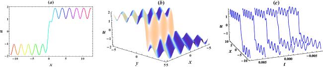
Figure 1. Profiles of the kink-cnoidal wave solution u given by equation ( |
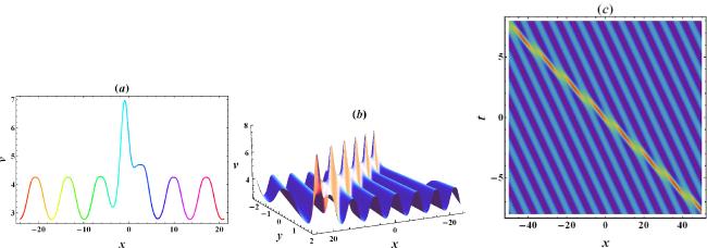
Figure 2. Profiles of the kink-cnoidal wave solution v in equation ( |
4. N-soliton solution and soliton molecules
Through a bi-logarithmic transformation1 ) with λ = 1 can be converted into the bilinear form
$\begin{eqnarray}u={\rm{i}}{\left(\mathrm{ln}\displaystyle \frac{{g}^{* }}{g}\right)}_{x},\quad v=-{\left(\mathrm{ln}{{gg}}^{* }\right)}_{{xy}},\end{eqnarray}$
where g and g* are complex functions of (x, y, t), the 2DmKdV system ( $\begin{eqnarray}\left\{\begin{array}{l}({D}_{t}+{D}_{x}^{2}{D}_{y}+\alpha {D}_{x}^{3}+\beta {D}_{x}^{5})g\cdot {g}^{* }=0,\\ {D}_{x}^{2}g\cdot {g}^{* }=0,\end{array}\right.\end{eqnarray}$
where the Hirota derivative is defined as $\begin{eqnarray*}\begin{array}{l}{D}_{t}^{m}{D}_{x}^{n}g\cdot f\\ \,={\left(\displaystyle \frac{\partial }{\partial {t}_{1}}-\displaystyle \frac{\partial }{\partial {t}_{2}}\right)}^{m}{\left(\displaystyle \frac{\partial }{\partial {x}_{1}}-\displaystyle \frac{\partial }{\partial {x}_{2}}\right)}^{n}g({x}_{1},{t}_{1})\cdot f({x}_{2},{t}_{2})\left|{}_{{x}_{1}={x}_{2},{t}_{1}={t}_{2}}\right..\end{array}\end{eqnarray*}$
To obtain the multiple soliton solution of the 2DmKdV system, we expand g and g* as power series with respect to a small parameter ε25 ) into (24 ) and then eliminating the coefficients of different powers of ε, we obtain the recursion relations (linear equation) of gi and ${g}_{i}^{* }$. Finally, it is found that N-soliton solutions can be obtained by taking
$\begin{eqnarray}\begin{array}{l}g=1+\epsilon {g}_{1}+{\epsilon }^{2}{g}_{2}+{\epsilon }^{3}{g}_{3}+\cdots ,\quad {g}^{* }=1+\epsilon {g}_{1}^{* }+{\epsilon }^{2}{g}_{2}^{* }\\ \,+\,{\epsilon }^{3}{g}_{3}^{* }+\cdots .\end{array}\end{eqnarray}$
Substituting ( $\begin{eqnarray}g=\displaystyle \sum _{\mu =0,1}\exp \left[\displaystyle \sum _{j=1}^{N}{\mu }_{j}\left({\xi }_{j}+{\rm{i}}\displaystyle \frac{\pi }{2}\right)+\displaystyle \sum _{1\leqslant j\lt l}^{N}{\mu }_{j}{\mu }_{l}{a}_{{jl}}\right],\end{eqnarray}$
where $\begin{eqnarray}\begin{array}{l}{\xi }_{j}={k}_{j}x+{l}_{j}y+{\omega }_{j}t,\quad {\omega }_{j}=-{k}_{j}^{2}({l}_{j}+\alpha {k}_{j}+\beta {k}_{j}^{3}),\\ \quad {{\rm{e}}}^{{a}_{{jl}}}={A}_{{jl}}=\displaystyle \frac{{\left({k}_{j}-{k}_{l}\right)}^{2}}{{\left({k}_{j}+{k}_{l}\right)}^{2}}.\end{array}\end{eqnarray}$
Case 1 for N = 1. In this case, choosing $g=1+{\mathrm{ie}}^{{\xi }_{1}}$ arrives at a one-soliton solution
$\begin{eqnarray}\begin{array}{l}u=-\displaystyle \frac{2{k}_{1}{{\rm{e}}}^{{\xi }_{1}}}{1+{{\rm{e}}}^{2{\xi }_{1}}}=-\displaystyle \frac{{k}_{1}}{\cosh ({\xi }_{1})},\\ \,\quad v=-\displaystyle \frac{4{k}_{1}{l}_{1}}{{\left(1+{{\rm{e}}}^{2{\xi }_{1}}\right)}^{2}}=-\displaystyle \frac{{k}_{1}{l}_{1}}{1+\cosh (2{\xi }_{1})}.\end{array}\end{eqnarray}$
Case 2 for N = 2. If $g=1+{\mathrm{ie}}^{{\xi }_{1}}+{\mathrm{ie}}^{{\xi }_{2}}-{A}_{12}{{\rm{e}}}^{{\xi }_{1}+{\xi }_{2}}$, then a two-soliton solution can be produced as
$\begin{eqnarray}u=-\displaystyle \frac{2({k}_{1}{{\rm{e}}}^{{\xi }_{1}}+{k}_{2}{{\rm{e}}}^{{\xi }_{2}})+2{A}_{12}({{\rm{e}}}^{{\xi }_{1}}+{{\rm{e}}}^{{\xi }_{2}}){{\rm{e}}}^{{\xi }_{1}+{\xi }_{2}}}{{\left(1-{A}_{12}{{\rm{e}}}^{{\xi }_{1}+{\xi }_{2}}\right)}^{2}+{\left({{\rm{e}}}^{{\xi }_{1}}+{{\rm{e}}}^{{\xi }_{2}}\right)}^{2}},\end{eqnarray}$
$\begin{eqnarray}v=-{\left\{\mathrm{ln}\left[{\left({{\rm{e}}}^{{\xi }_{1}}+{{\rm{e}}}^{{\xi }_{2}}\right)}^{2}+{\left(1-{A}_{12}{{\rm{e}}}^{{\xi }_{1}+{\xi }_{2}}\right)}^{2}\right]\right\}}_{{xy}}.\end{eqnarray}$
Figure 3(a) presents a two-soliton structure of the solution u. It is known that a soliton molecule can be obtained from the two-soliton solution by imposing a velocity resonance condition [17]. Here, the following type of the resonance conditions is introduced
$\begin{eqnarray}\displaystyle \frac{{k}_{i}}{{k}_{j}}=\displaystyle \frac{{l}_{i}}{{l}_{j}}=\displaystyle \frac{{\omega }_{i}}{{\omega }_{j}},\quad {k}_{i}\ne \pm {k}_{j},\quad {l}_{i}\ne \pm {l}_{j},\end{eqnarray}$
which requires $\begin{eqnarray}{l}_{1}=\alpha {k}_{1}-\beta {k}_{1}({k}_{1}^{2}+{k}_{2}^{2}),\quad {l}_{2}=\alpha {k}_{2}-\beta {k}_{2}({k}_{1}^{2}+{k}_{2}^{2}).\end{eqnarray}$
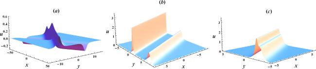
Figure 3. Profiles of the wave solution u given by ( |
With the above parameter values (32 ), the two-soliton solution (29 ) becomes a soliton molecule, which is graphically displayed in figure 3(b) and (c). It is obviously observed from figure 3(b) that, despite the equal velocity, the height and width of the two peaks in the soliton molecule are visibly different. Additionally, the distance between the two peaks is determined by the phase constants ξi0. It is noted that, under suitable values of the phase constants, the two peaks of the molecule can get close enough to each other, and thus leads to the formation of an asymmetric soliton as exhibited in figure 3(c).
Case 3 for N = 3. In this case, the explicit form of g reads33 ) into (23 ), one can immediately obtain the three-soliton solution as shown in figure 4(a). Here, we omit the lengthy expressions of the wave solutions. Similarly, by imposing the velocity resonance condition (31 ) on the first two solitons, we find ${l}_{1}=-{k}_{1}[\alpha +\beta ({k}_{1}^{2}+{k}_{2}^{2})]$ and ${l}_{2}=-{k}_{2}[\alpha +\beta ({k}_{1}^{2}+{k}_{2}^{2})]$. Consequently, the interaction between one soliton and one two-soliton molecule is produced, as shown in figure 4(b), and the corresponding space-time evolution is displayed in figure 4(c).
$\begin{eqnarray}\begin{array}{l}g=1+{\rm{i}}({{\rm{e}}}^{{\xi }_{1}}+{{\rm{e}}}^{{\xi }_{2}}+{{\rm{e}}}^{{\xi }_{3}})-{A}_{12}{{\rm{e}}}^{{\xi }_{1}+{\xi }_{2}}-{A}_{13}{{\rm{e}}}^{{\xi }_{1}+{\xi }_{3}}\\ \,-{A}_{23}{{\rm{e}}}^{{\xi }_{2}+{\xi }_{3}})-{\rm{i}}{A}_{12}{A}_{13}{A}_{23}{{\rm{e}}}^{{\xi }_{1}+{\xi }_{2}+{\xi }_{3}}.\end{array}\end{eqnarray}$
By substituting (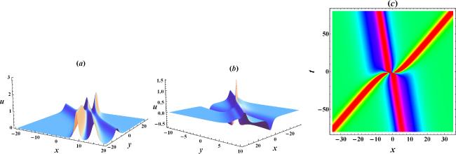
Figure 4. (a) 3D plot of the three-soliton solution u with k1 = 1.5, k2 = 1, k3 = 0.5, l1 = l2 = l3 = 0.5, ξ10 = ξ20 = ξ30 = 0, α = 0.2 and β = 0.04. (b) 3D plot of the soliton-asymmetric soliton solution with k1 = 0.25, k2 = 0.75, k3 = –0.5, l3 = 0.5, ξ10 = ξ20 = 0, ξ30 = –3, α = 2 and β = 2. (c) Density plot of the space-time evolution of the soliton-asymmetric soliton interaction. |
Case 4 for N = 4. Now we have a four-soliton solution with g given by
$\begin{eqnarray}\begin{array}{rcl}g & = & 1+{\rm{i}}({{\rm{e}}}^{{\xi }_{1}}+{{\rm{e}}}^{{\xi }_{2}}+{{\rm{e}}}^{{\xi }_{3}}+{{\rm{e}}}^{{\xi }_{4}})-{A}_{12}{{\rm{e}}}^{{\xi }_{1}+{\xi }_{2}}-{A}_{13}{{\rm{e}}}^{{\xi }_{1}+{\xi }_{3}}\\ & & -\,{A}_{14}{{\rm{e}}}^{{\xi }_{1}+{\xi }_{4}}-{A}_{23}{{\rm{e}}}^{{\xi }_{2}+{\xi }_{3}}-{A}_{24}{{\rm{e}}}^{{\xi }_{2}+{\xi }_{4}}-{A}_{34}{{\rm{e}}}^{{\xi }_{3}+{\xi }_{4}}\\ & & -\,{\rm{i}}{A}_{12}{A}_{13}{A}_{23}{{\rm{e}}}^{{\xi }_{1}+{\xi }_{2}+{\xi }_{3}}-{\rm{i}}{A}_{12}{A}_{14}{A}_{24}{{\rm{e}}}^{{\xi }_{1}+{\xi }_{2}+{\xi }_{4}}\\ & & -\,{\rm{i}}{A}_{13}{A}_{14}{A}_{34}{{\rm{e}}}^{{\xi }_{1}+{\xi }_{3}+{\xi }_{4}}-{\rm{i}}{A}_{23}{A}_{24}{A}_{34}{{\rm{e}}}^{{\xi }_{2}+{\xi }_{3}+{\xi }_{4}}\\ & & +\,{A}_{12}{A}_{13}{A}_{14}{A}_{23}{A}_{24}{A}_{34}{{\rm{e}}}^{{\xi }_{1}+{\xi }_{2}+{\xi }_{3}+{\xi }_{4}}.\end{array}\end{eqnarray}$
Clearly, the larger the N, the more abundant the patterns of soliton molecules provided by the solution. For instance, applying the velocity resonance condition (31 ) on two pairs of solitons, respectively, arrives at
$\begin{eqnarray}\begin{array}{rcl} & & {l}_{1}=-{k}_{1}[\alpha +\beta ({k}_{1}^{2}+{k}_{2}^{2})],\quad {l}_{2}=-{k}_{2}[\alpha +\beta ({k}_{1}^{2}+{k}_{2}^{2})],\\ & & \,{l}_{3}=-{k}_{3}[\alpha +\beta ({k}_{3}^{2}+{k}_{4}^{2})],\quad {l}_{4}=-{k}_{4}[\alpha +\beta ({k}_{3}^{2}+{k}_{4}^{2})].\end{array}\end{eqnarray}$
Thereafter, the four-soliton solution degenerates into two two-soliton molecules, as shown in figure 5(a), where one group of parallel lines, representing a two-soliton molecule, intersects elastically with the other group of parallel lines representing the other two-soliton molecule. Similar to the previous situation, suitable choices of the phase constants ξi0 will lead to an elastic interaction between two asymmetric solitons, as exhibited in figure 5(b). It is interesting to remark that two peaks embedded in an asymmetric soliton will get separated from each other after the interaction. In addition, one can also construct a special soliton molecule which is a bound state of two solitons and one breather, as shown in figure 5(c). To construct such a soliton molecule, we restrict $\begin{eqnarray}\begin{array}{rcl}{k}_{3} & = & {K}_{r}+{\rm{i}}{K}_{i},\quad {k}_{4}={K}_{r}-{\rm{i}}{K}_{i},\\ & & \quad {l}_{3}={L}_{r}+{\rm{i}}{L}_{i},\quad {l}_{4}={L}_{r}-{\rm{i}}{L}_{i},\\ & & \,{\omega }_{3}={{\rm{\Omega }}}_{r}+{\rm{i}}{{\rm{\Omega }}}_{i},\\ & & \quad {\omega }_{4}={{\rm{\Omega }}}_{r}-{\rm{i}}{{\rm{\Omega }}}_{i},\quad {\xi }_{30}={\xi }_{40}=0,\end{array}\end{eqnarray}$
where Ωr and Ωi satisfy the following dispersion relation $\begin{eqnarray}\begin{array}{rcl} & & {{\rm{\Omega }}}_{r}=\alpha {K}_{r}(3{K}_{i}^{2}-{K}_{r}^{2})-\beta {K}_{r}(5{K}_{i}^{4}-10{K}_{r}^{2}{K}_{i}^{2}+{K}_{r}^{4})\\ & & \,+{L}_{r}({K}_{i}^{2}-{K}_{r}^{2}),\\ & & {{\rm{\Omega }}}_{i}=-\alpha {K}_{i}(3{K}_{r}^{2}-{K}_{i}^{2})-\beta {K}_{i}(5{K}_{r}^{4}-10{K}_{r}^{2}{K}_{i}^{2}+{K}_{i}^{4})\\ & & \,-2{K}_{r}{K}_{i}{L}_{r}.\end{array}\end{eqnarray}$
The introduction of the velocity resonance conditions ω1/k1 = ω2/k2 = Ωr/Kr and ω1/l1 = ω2/l2 = Ωr/Lr leads to $\begin{eqnarray}\begin{array}{l}{l}_{1}=-{k}_{1}[\alpha +\beta ({k}_{1}^{2}+{k}_{2}^{2})],\ {l}_{2}=-{k}_{2}[\alpha +\beta ({k}_{1}^{2}+{k}_{2}^{2})],{L}_{r}=-{K}_{r}[\alpha +\beta ({k}_{1}^{2}+{k}_{2}^{2})],\\ {L}_{i}=\displaystyle \frac{-2\alpha {k}_{1}^{2}+\beta [5{K}_{i}^{4}+{K}_{i}^{2}({k}_{1}^{2}+{k}_{2}^{2}-10{K}_{r}^{2})+({K}_{r}^{2}-{k}_{1}^{2})({K}_{r}^{2}-{k}_{3}^{2})]}{2{K}_{i}}.\end{array}\end{eqnarray}$
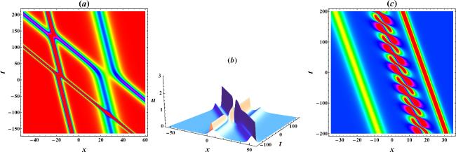
Figure 5. The soliton molecule patterns from the four soliton solution. (a) The density plot of the space-time evolution of two two-soliton molecules with k1 = –1.5, k2 = –0.4, k3 = –0.9, k4 = –0.3, ξ10 = –ξ20 = –15, ξ30 = − ξ40 = –10, α = 0.5 and β = 1. (b) 3D plot of the interaction between two asymmetric solitons with the same parameters as (a), except for ξ10 = –ξ20 = 0.25, ξ30 = 0 and ξ40 = 4.5. (c) The density plot of the space-time evolution of a special soliton molecule with k1 = 1, k2 = 0.5, Kr = 0.75, Ki = –0.25, ξ10 = –ξ20 = –10, α = 0.5 and β = 0.25 |
5. Conclusions and discussions
In summary, several aspects of the 2DmKdV system are studied. Based on the truncated Painlevé expansion method, we obtain the nonlocal residue symmetry and the Bäcklund transformation. The nonlocal symmetry is thus localized to the Lie point symmetry of the enlarged system via introducing several new auxiliary functions. By virtue of the CTE method, the soliton-cnoidal wave solutions are explicitly presented and graphically displayed. Finally, several types of soliton molecules are illustrated, such as the asymmetric soliton and the soliton-breather molecule, which are produced from the N-soliton solution through a velocity resonance mechanism. It is hoped that the explicit solutions obtained here may find their physical applications in the near future.